Comparative Assessment of Hierarchical Clustering Methods for Grouping in Singular Spectrum Analysis

Abstract

Singular spectrum analysis (SSA) is a popular filtering and forecasting method that is used in a wide range of fields such as time series analysis and signal processing. A commonly used approach to identify the meaningful components of a time series in the grouping step of SSA is the utilization of the visual information of eigentriples. Another supplementary approach is that of employing an algorithm that performs clustering based on the dissimilarity matrix defined by weighted correlation between the components of a time series. The SSA literature search revealed that no investigation has compared the various clustering methods. The aim of this paper was to compare the effectiveness of different hierarchical clustering linkages to identify the appropriate groups in the grouping step of SSA. The comparison was performed based on the corrected Rand (CR) index as a comparison criterion that utilizes various simulated series. It was also demonstrated via two real-world time series how one can proceed, step-by-step, to conduct grouping in SSA using a hierarchical clustering method. This paper is supplemented with accompanying R codes.

1. Introduction

Singular spectrum analysis (SSA) is a model-free technique that decomposes a time series into a number of meaningful components. Owing to its widespread applications in various fields, this non-parametric method has received much attention in recent years. As evidence, examples of the wide variety of SSA applications can be found in [1,2,3,4,5,6,7,8,9]. A whole and precise detailed summary of the theory and applications of SSA can be found in [10,11]. Additionally, there are other books devoted to SSA; for example, Refs. [12,13,14]. A comprehensive review of SSA and the description of its modifications and extensions can be found in [15].

One of the challenging problems of SSA is identifying the interpretable components of a time series. The conventional method of detecting interpretable components such as trend and periodic components, is to apply the information contained in singular values and singular vectors of the trajectory matrix of a time series. In this approach, a screen plot of the singular values, one-dimensional and two-dimensional figures of the singular vectors, and the matrix of the absolute values of the weighted correlations can provide a visual method to identify the appropriate components. More details on group identification based on visual tools can be found in [11,14].

There is another supplementary approach to identifying the meaningful components of a time series that performs clustering based on a dissimilarity matrix defined by weighted correlation between elementary components. In this simple method, first, the similarity of elementary components is measured by means of the weighted correlations between them. Then, a proximity matrix is constructed using weighted correlations. Finally, the elementary components are grouped via distance-based clustering techniques such as hierarchical methods. Although this approach is interesting, it has not yet been established which hierarchical clustering method can provide an accurate and reasonable grouping. For instance, the hierarchical clustering with complete linkage was used in [16], while the reason for selecting the complete linkage was not clear. Since, to the best of our knowledge, no one has conducted a comparison study to determine an adequate hierarchical clustering method on the basis of weighted correlations, the present research has tried to fill this gap. In this investigation, we sought to compare the performance of several hierarchical clustering linkages in order to find a proper linkage.

This paper is divided into five sections. In Section 2, the theoretical background and general scheme of basic SSA are reviewed. Furthermore, a brief overview of hierarchical clustering methods and measure of similarity between clusters that is exploited in this research is outlined in this section. Section 3 is dedicated to comparing the performance of hierarchical clustering linkages via simulating a variety of synthetic time series. Two case studies are proposed in Section 4 using real-world time series datasets. In this section, it is also demonstrated how one can proceed, step-by-step, to conduct grouping in SSA using a hierarchical clustering method. Some conclusions and the discussion are given in Section 5 and supplementary R codes are presented in the Appendix A.

2. Theoretical Background

In this section, we first briefly explain the theory underlying Basic SSA which is the most fundamental version of the SSA technique. Then, the hierarchical clustering methods that are of interest to this study were reviewed.

2.1. Review of Basic SSA

The basic SSA consists of four steps which are similar to those of other versions of SSA. These steps are briefly described below and in doing so, we mainly follow [11,14]. More detailed information on the theory of the SSA method can be found in [10].

Step 1: 

Embedding. In this step, the time series $\mathbb{X}=\{x_1,\dots ,x_N\}$ is transformed into the $L\times K$ matrix $\mathbf{X}$, whose columns comprise $X_1,\dots ,X_K$, where $X_i={(x_i,\dots ,x_{i+L-1})}^T$$\in {\mathbb{R}}^L$ and $K=N-L+1$. The matrix $\mathbf{X}$ is called the trajectory matrix. This matrix is a Hankel matrix in the sense that all the elements on the anti-diagonals $i+j=const.$ are equal. The embedding step only has one parameter L, which is called the window length or embedding dimension. The window length is commonly chosen such that $2\le L\le N/2$ where N is the length of the time series $\mathbb{X}$.

Step 2: 

Decomposition. In this step, the trajectory matrix $\mathbf{X}$ is decomposed into a sum of rank-one matrices using the conventional singular value decomposition (SVD) procedure. The eigenvalues of $\mathbf{X}{\mathbf{X}}^T$ were denoted by ${\lambda }_1,\dots ,{\lambda }_L$ in decreasing order of magnitude $\left({\lambda }_1\ge \cdots \ge {\lambda }_L\ge 0\right)$ and by $U_1,\dots ,U_L$, the eigenvectors of the matrix $\mathbf{X}{\mathbf{X}}^T$ corresponding to these eigenvalues. If $d=\max \{i,\mathrm{such}\mathrm{that}{\lambda }_i>0\}=rank\left(\mathbf{X}\right)$, then the SVD of the trajectory matrix can be written as

$$\mathbf{X}={\mathbf{X}}_1+\cdots +{\mathbf{X}}_d,$$

(1)

where ${\mathbf{X}}_i={\sqrt{\lambda }}_i{U}_i{V_i}^T$ and $V_i={\mathbf{X}}^T{U}_i/{\sqrt{\lambda }}_i$ ($i=1,\dots ,d$). The collection ($\sqrt{{\lambda }_i},U_i,V_i$) is called the ith eigentriple of the SVD.

Step 3: 

Grouping. The aim of this step is to group the components of (1). Let $I=\{i_1,\dots ,i_p\}$ be the subset of indices $\{1,\dots ,d\}$. Then, the resultant matrix ${\mathbf{X}}_I$ corresponding to the group I is defined as ${\mathbf{X}}_I={\mathbf{X}}_{i_1}+\cdots +{\mathbf{X}}_{i_p}$, that is, summing the matrices within each group. With the SVD of $\mathbf{X}$, the split of the set of indices $\{1,\dots ,d\}$ into the m disjoint subsets $I_1,\dots ,I_m$ corresponds to the following decomposition:

$$\mathbf{X}={\mathbf{X}}_{I_1}+\cdots +{\mathbf{X}}_{I_m}.$$

(2)

If $I_i=\left\{i\right\}$, for $i=1,\dots ,d$, then the corresponding grouping is called elementary.

Step 4: 

Diagonal Averaging. The main goal of this step is to transform each matrix ${\mathbf{X}}_{I_j}$ of the grouped matrix decomposition (2) into a Hankel matrix, which can subsequently be converted into a new time series of length N. Let $\mathbf{A}$ be an $L\times K$ matrix with elements $a_{ij}$, $1\le i\le L,1\le j\le K$. By diagonal averaging, the matrix $\mathbf{A}$ is transferred into the Hankel matrix $\mathcal{H}\mathbf{A}$ with the elements ${\tilde{a}}_s$ over the anti-diagonals $(1\le s\le N)$ using the following formula:

$${\tilde{a}}_s=\sum _{(l,k)\in A_s}\frac{a_{lk}}{|A_s|},$$

(3)

where $A_s=\{(l,k):l+k=s+1,1\le l\le L,1\le k\le K\}$ and $|A_s|$ denotes the number of elements in the set $A_s$. By applying diagonal averaging (3) to all the matrix components of (2), the following expansion is obtained: $\mathbf{X}={\tilde{\mathbf{X}}}_{I_1}+\cdots +{\tilde{\mathbf{X}}}_{I_m},$ where ${\tilde{\mathbf{X}}}_{I_j}=\mathcal{H}{\mathbf{X}}_{I_j}$, $j=1,\cdots ,m$. This is equivalent to the decomposition of the initial series $\mathbb{X}=\{x_1,\dots ,x_N\}$ into a sum of m series: $x_t={\sum }_{k=1}^m{\tilde{x}}_t^{\left(k\right)}(t=1,\dots ,N)$, where ${\tilde{\mathbb{X}}}_k=\{{\tilde{x}}_1^{\left(k\right)},\dots ,{\tilde{x}}_N^{\left(k\right)}\}$ corresponds to the matrix ${\tilde{\mathbf{X}}}_{I_k}$.

Usually, Steps 1 and 2 of the SSA technique are called the Decomposition Stage, and Steps 3 and 4 are called the Reconstruction Stage. There are many software applications to implement SSA such as Caterpillar-SSA and SAS/ETS. In this investigation, we apply the free available R package Rssa to conduct the decomposition and reconstruction stages of SSA. More details on this package can be found in [17,18,19].

There is a fundamental concept in SSA called separability that indicates the quality of the decomposition by determining how well different components of a time series are separated from each other. Let us describe this important concept in more detail. Let $\mathbf{A}={\left\{a_{ij}\right\}}_{i,j=1}^{L,K}$ and $\mathbf{B}={\left\{b_{ij}\right\}}_{i,j=1}^{L,K}$ be $L\times K$ matrices. The inner product of two matrices $\mathbf{A}$ and $\mathbf{B}$ is defined as

$$\langle \mathbf{A},\mathbf{B}\rangle =\sum _{i=1}^L\sum _{j=1}^K{a}_{ij}{b}_{ij}.$$

Based on this definition of inner product, the Frobenius norm of matrices $\mathbf{A}$ and $\mathbf{B}$ is ${∥\mathbf{A}∥}_F=\sqrt{\langle \mathbf{A},\mathbf{A}\rangle }$, ${∥\mathbf{B}∥}_F=\sqrt{\langle \mathbf{B},\mathbf{B}\rangle }$. Now, suppose that ${\tilde{\mathbf{X}}}_i=\mathcal{H}{\mathbf{X}}_i$ and ${\tilde{\mathbf{X}}}_j=\mathcal{H}{\mathbf{X}}_j$ are, respectively, the trajectory matrices of two reconstructed series ${\tilde{\mathbb{X}}}_i$ and ${\tilde{\mathbb{X}}}_j$, which are obtained from the diagonal averaging step of SSA based on the elementary grouping $I_i=\left\{i\right\}$. The measure of approximate separability between two reconstructed series ${\tilde{\mathbb{X}}}_i$ and ${\tilde{\mathbb{X}}}_j$ is the weighted correlation or w-correlation, which is defined as

$${\rho }_{ij}^{\left(\mathbf{w}\right)}=\frac{〈{\tilde{\mathbf{X}}}_i,{\tilde{\mathbf{X}}}_j〉}{{∥{\tilde{\mathbf{X}}}_i∥}_F{∥{\tilde{\mathbf{X}}}_j∥}_F}.$$

Geometrically, ${\rho }_{ij}^{\left(\mathbf{w}\right)}$ is equal to the cosine of the angle between the two trajectory matrices of reconstructed components ${\tilde{\mathbb{X}}}_i$ and ${\tilde{\mathbb{X}}}_j$. Using the Hankel property of matrices ${\tilde{\mathbf{X}}}_i$ and ${\tilde{\mathbf{X}}}_j$, it can be easily shown that the w-correlation is equivalent to the following form [10]:

$${\rho }_{ij}^{\left(\mathbf{w}\right)}=\frac{{\sum }_{k=1}^N{w}_k{x}_k^{\left(i\right)}{x}_k^{\left(j\right)}}{\sqrt{{\sum }_{k=1}^N{w}_k{\left(x_k^{\left(i\right)}\right)}^2}\sqrt{{\sum }_{k=1}^N{w}_k{\left(x_k^{\left(j\right)}\right)}^2}},$$

(4)

where $w_k=min\{k,L,N-k+1\}$. It is noteworthy that the weight $w_i$ is equal to the number of times the element $x_i$ appears in the trajectory matrix $\mathbf{X}$ of the initial time series $\mathbb{X}=\{x_1,\dots ,x_N\}$. If ${\rho }_{ij}^{\left(\mathbf{w}\right)}$ is large, then it can be deduced that ${\tilde{\mathbb{X}}}_i$ and ${\tilde{\mathbb{X}}}_j$ are highly correlated. Hence, these two components should be included in the same group. However, a small value of the w-correlation can indicate the good separability of the components. Consequently, an absolute value of the w-correlation close to zero ($\left|{\rho }_{ij}^{\left(\mathbf{w}\right)}\right|\simeq 0$) would imply a high separation between two reconstructed components ${\tilde{\mathbb{X}}}_i$ and ${\tilde{\mathbb{X}}}_j$.

2.2. Hierarchical Clustering Methods

In this paper, we apply hierarchical clustering methods to cluster the eigentriples in the grouping step of SSA. Hierarchical clustering is a widely used clustering method that connects objects to form clusters based on their distance. This distance-based method requires the definition of a dissimilarity measure (or distance) between objects. There is a multitude of dissimilarity measures available in the literature that can be used in hierarchical clustering, such as Euclidean, Manhattan, Canberra, Minkowski, binary and maximum distances. Owing to the fact that different distances result in different clusters, some important aspects should be considered in the choice of the similarity measure. The main considerations include the nature of the variables (discrete, continuous, binary), the scales of measurement (nominal, ordinal, interval, ratio), and subject matter knowledge [20]. In this article, we define the dissimilarity measure between the two reconstructed components ${\tilde{\mathbb{X}}}_i$ and ${\tilde{\mathbb{X}}}_j$ as $d_{ij}=1-\left|{\rho }_{ij}^{\left(\mathbf{w}\right)}\right|$. As illustrated in [14], the Algorithm 1 of auto-grouping based on clustering methods can be written as follows:

Algorithm 1 Auto-grouping using clustering methods.

Require:  Time series $\mathbb{X}=\{x_1,\dots ,x_N\}$, window length (L), number of groups;  1: Decompose time series into elementary components.  2: Compute w-correlation (${\rho }_{ij}^{\left(\mathbf{w}\right)}$) between elementary reconstructed series ${\tilde{\mathbb{X}}}_i$ and ${\tilde{\mathbb{X}}}_j$ using (4).  3: Compute dissimilarity between elementary reconstructed series ${\tilde{\mathbb{X}}}_i$ and ${\tilde{\mathbb{X}}}_j$ as $d_{ij}=1-\left|{\rho }_{ij}^{\left(\mathbf{w}\right)}\right|$.  4: Construct the distance matrix $\mathbf{D}=\left[d_{ij}\right]$.  5: Use a method of clustering to the distance matrix $\mathbf{D}$.  6: Obtain the given number of groups from the results of cluster analysis.

It should be noted that the automatic identification of SSA components has a limitation. As mentioned in [11], this limitation is assuming that the components to be identified are (approximately) separated from the rest of the time series.

There are generally two types of hierarchical clustering approaches:

• Divisive. In this approach, an initial single cluster of objects is divided into two clusters such that the objects in one cluster are far from the objects in the other cluster. The process proceeds by splitting the clusters into smaller and smaller clusters until each object forms a separate cluster [20,21]. We implemented this method in our research via the function diana from the cluster package [22] of the freely available statistical R software [23].
• Agglomerative. In this approach, the individual objects are initially treated as a cluster, and then the most similar clusters are merged according to their similarities. This procedure proceeds by successive fusions until a single cluster is eventually obtained containing all the objects [20,21]. Several agglomerative hierarchical clustering methods are employed in this paper including single, complete, average, mcquitty, median, centroid and Ward. There are two algorithms ward.D and ward.D2 for the Ward method, which are available in R packages such as stats and NbClust [24]. By implementing the ward.D2 algorithm, the dissimilarities are squared before the cluster updates.

All of the agglomerative hierarchical clustering methods that were implemented in this research can be attained via the function hclust from the stats package of R software. More information about hierarchical clustering algorithms can be found in [20,21,25,26].

2.3. Cluster Validation Measure

In this paper, we used the corrected Rand (CR) index to measure the similarity between the grouping output obtained with a hierarchical clustering method and a given “correct” grouping. Let us explain the CR index in more detail. Given an n element set S, suppose $X=\left\{X_1,X_2,\dots ,X_r\right\}$ and $Y=\left\{Y_1,Y_2,\dots ,Y_c\right\}$ represent two different partitions of S. The information on class overlap between the two partitions X and Y can be written in the form of

Table 1. Notations for the CR index.

	${\mathit{Y}}_1$	${\mathit{Y}}_2$	⋯	${\mathit{Y}}_{\mathit{c}}$	sums
$X_1$	$n_{11}$	$n_{12}$	⋯	$n_{1c}$	$n_{1·}$
$X_2$	$n_{21}$	$n_{22}$	⋯	$n_{2c}$	$n_{2·}$
⋮	⋮	⋮	⋱	⋮	⋮
$X_r$	$n_{r1}$	$n_{r2}$	⋯	$n_{rc}$	$n_{r·}$
sums	$n_{·1}$	$n_{·2}$	⋯	$n_{·c}$	$n=n_{··}$

:

Where $n_{ij}$ denotes the number of objects that are common to classes $X_i$ and $Y_j$, $n_{i·}$ and $n_{·j}$ refer, respectively, to the number of objects in classes $X_i$ (sum of row i) and $Y_j$ (sum of column j). Based on the notations provided in Table 1, the CR index is defined as follows:

$$CR=\frac{{\sum }_{ij}\left(\genfrac{}{}{0pt}{}{n_{ij}}{2}\right)-{\sum }_i\left(\genfrac{}{}{0pt}{}{n_{i·}}{2}\right){\sum }_j\left(\genfrac{}{}{0pt}{}{n_{·j}}{2}\right)/\left(\genfrac{}{}{0pt}{}{n}{2}\right)}{\frac{1}{2}\left[{\sum }_i\left(\genfrac{}{}{0pt}{}{n_{i·}}{2}\right)+{\sum }_j\left(\genfrac{}{}{0pt}{}{n_{·j}}{2}\right)\right]-{\sum }_i\left(\genfrac{}{}{0pt}{}{n_{i·}}{2}\right){\sum }_j\left(\genfrac{}{}{0pt}{}{n_{·j}}{2}\right)/\left(\genfrac{}{}{0pt}{}{n}{2}\right)}$$

The CR index is an external cluster validation index and can be implemented in the R function cluster.stats from the fpc package [27]. This index varies from −1 (no similarity) to 1 (perfect similarity) and if it displays high values then this indicates great similarity between the two clusters. However, this index does not take into consideration the numbers and contributions of time series components with the wrong partition. More details on this index can be found in [25,28,29,30].

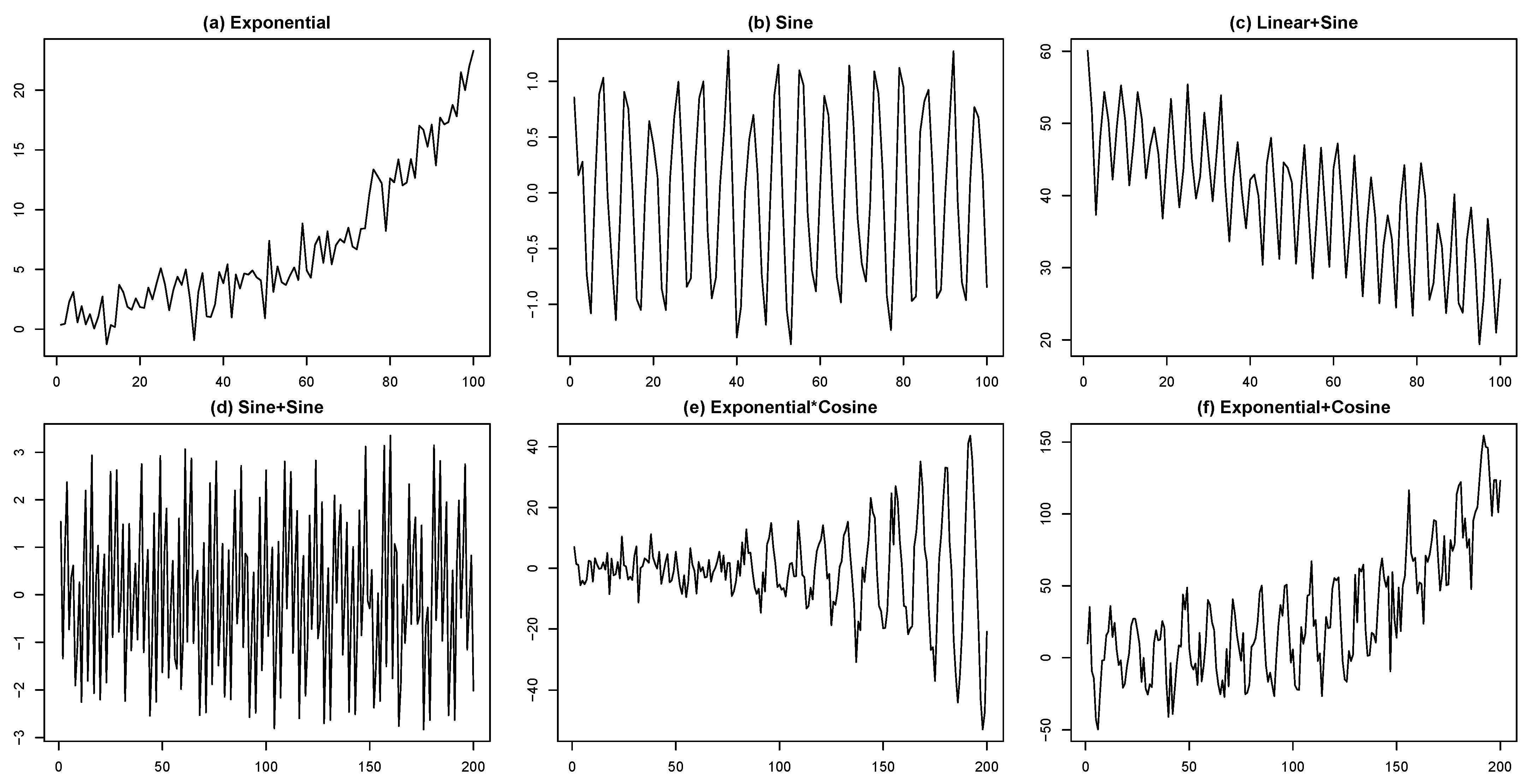
3. Simulation Study

In this section, the performances of agglomerative and divisive hierarchical clustering methods were evaluated by applying them to various simulated time series with different patterns. In the following simulated series, the normally distributed noise with zero mean (${\epsilon }_t$) is added to each point of the generated series:

(a)

Exponential:$y_t=exp\left(0.03t\right)+{\epsilon }_t,t=1,2,\dots ,100$

(b)

Sine:$y_t=sin(2\pi t/6)+{\epsilon }_t,t=1,2,\dots ,100$

(c)

Linear + Sine:$y_t=50-0.2t+8sin(2\pi t/4)+{\epsilon }_t,t=1,2,\dots ,100$

(d)

Sine + Sine:$y_t=2sin(2\pi t/3)+sin(2\pi t/12)+{\epsilon }_t,t=1,2,\dots ,200$

(e)

Exponential × Cosine:$y_t=exp\left(0.02t\right)cos(2\pi t/12)+{\epsilon }_t,t=1,2,\dots ,200$

(f)

Exponential + Cosine:$y_t=exp\left(0.025t\right)+30cos(2\pi t/12)+{\epsilon }_t,t=1,2,\dots ,200$

Various signal-to-noise ratios (SNRs) including $0.25,0.75,5,$ and 10 were employed to assess the impact of noise levels on grouping results. The simulation was repeated 5000 times for each SNR of each scenario (a)–(f) and then, the average of the CR index was computed. In order to enable better comparison, the dashed horizontal line $y=1$ was added to all figures of the CR index. To observe the structure of each simulated series, the simulation was performed once with $SNR=10$. The time series plots of the simulated series are depicted in Figure 1. As can be seen in this figure, the simulated series (a)–(f) have various patterns such as an upward and downward trends, and periodicity.

In

Table 2. Correct groups of the simulated series.

Simulated Series	Correct Groups	The Number of Clusters
Exponential	$\left\{1\right\},\{2,\dots ,L\}$	2
Sine	$\{1,2\},\{3,\dots ,L\}$	2
Linear+sine	$\{1,2\},\{3,4\},\{5,\dots ,L\}$	3
Sine+Sine	$\{1,2\},\{3,4\},\{5,\dots ,L\}$	3
Exponential×Cosine	$\{1,2\},\{3,\dots ,L\}$	2
Exponential+Cosine	$\left\{1\right\},\{2,3\},\{4,\dots ,L\}$	3

, the “correct” groups for each of the simulated series are determined based on the rank of the trajectory matrix of the simulated series and the grouping rules proposed in [10]. A major step in hierarchical clustering is the decision on where to cut the dendrogram. In this simulation study, we used the number of groups (or clusters), which is reported in Table 2, as a cutting rule of the dendrogram.

Figure 2 shows the CR index for the exponential series (case a) which are computed for various hierarchical clustering algorithms and different values of window length (L). It can be concluded from this figure that the ward.D and ward.D2 methods have the worst performance at each level of SNR. In addition, the similarity between the grouping by the complete method and “correct” groups decrease as L increases. However, the other methods exhibit good performance in detecting the “correct” groups, especially for a larger SNR. In the case of $SNR=0.25$, the methods of centroid, single, and average are better than the methods of mcquitty, median, and diana.

Figure 3 depicts the CR index for the Sine series (case b). It can be deduced from this figure that the ward.D and ward.D2 methods are unable to identify the “correct” groups at each level of the SNR when $L\ge 18$. In addition, it seems that the capability of the complete method to increase as the SNR reaches high levels, although its capability for moderate values of L is better than other values when $SNR>1$. Moreover, the diana method generally outperforms the ward.D, ward.D2, and complete methods. When $SNR<1$, the methods of centroid, single, and average provide more reliable outputs compared to the mcquitty, median, and diana methods. Furthermore, it seems that there is not a significant difference among the centroid, single, average, and mcquitty techniques when $SNR>1$.

In Figure 4, the CR index for the Linear+Sine series (case c) is presented. Once again, it can be concluded from this figure that the ward.D and ward.D2 methods have the worst performance at each level of SNR. The other results that can be concluded from this figure are similar to those of the Sine series (case b) and are hence not repeated here.

As we can see in Figure 4, the CR index of any of the methods could not obtain the value of one. This is true for all cases of SNR. In other words, none of the methods could exactly identify the correct groups at each level of SNR. This is due to the fact that the rank of linear time series is equal to 2 and therefore, it generates two non-zero eigenvalues. However, the second eigenvalue of the linear time series is relatively small and consequently, it is probably mixed with noise and can therefore not be identified, especially for a high level of noise.

In Figure 5, the CR index for the Sine+Sine series (case d) is shown. Once again, the ward.D and ward.D2 methods present poor results at each level of the SNR. When $SNR<1$, the single, centroid and average methods provide better results in comparison to the other methods. Furthermore, it seems that these methods can exactly identify the correct groups if $SNR>1$.

Figure 6 depicts the CR index for the Exponential×Cosine series (case e). As can be seen in this figure, the ward.D and ward.D2 methods cannot detect the “correct” groups at each level of the SNR. The single and average methods show better outputs when $SNR<1$. Additionally, in the case of $SNR>1$, it seems that there is not a significant difference among the single, average, and mcquitty approaches.

In Figure 7, the CR index for the Exponential+Cosine series (case f) is presented. Similar to the previous results, the ward.D and ward.D2 methods cannot provide effective results at each level of the SNR. However, it seems that the centroid, single, and average methods are better than the other methods—especially for $SNR<1$.

The outputs of the simulation study clearly indicate that the ward.D and ward.D2 methods cannot detect the “correct” groups at each level of the SNR. In addition, these outputs reveal that choosing the best hierarchical clustering linkage is not straightforward—it depends on the structure of a time series and the level of the contribution of noise. In order to have a general overview of the simulation results, the findings of the simulation study are summarized in

Table 3. Proper linkages based on the simulation results.

Simulated Series	Proper Linkages
Exponential	average, centroid, diana, mcquitty, median, single
Sine	average, centroid, mcquitty, median, single
Linear + sine	average, centroid, mcquitty, median, single
Sine + Sine	average, centroid, mcquitty, median, single
Exponential × Cosine	average, single, mcquitty
Exponential + Cosine	average, centroid, single

. Based on these findings, it seems that the single, centroid, average and mcquitty methods can identify the “correct” groups better than the other linkages.

4. Case Studies

Here, let us apply the hierarchical clustering methods to identify adequate groups using real-world datasets. To this end, two time series datasets were considered as follows:

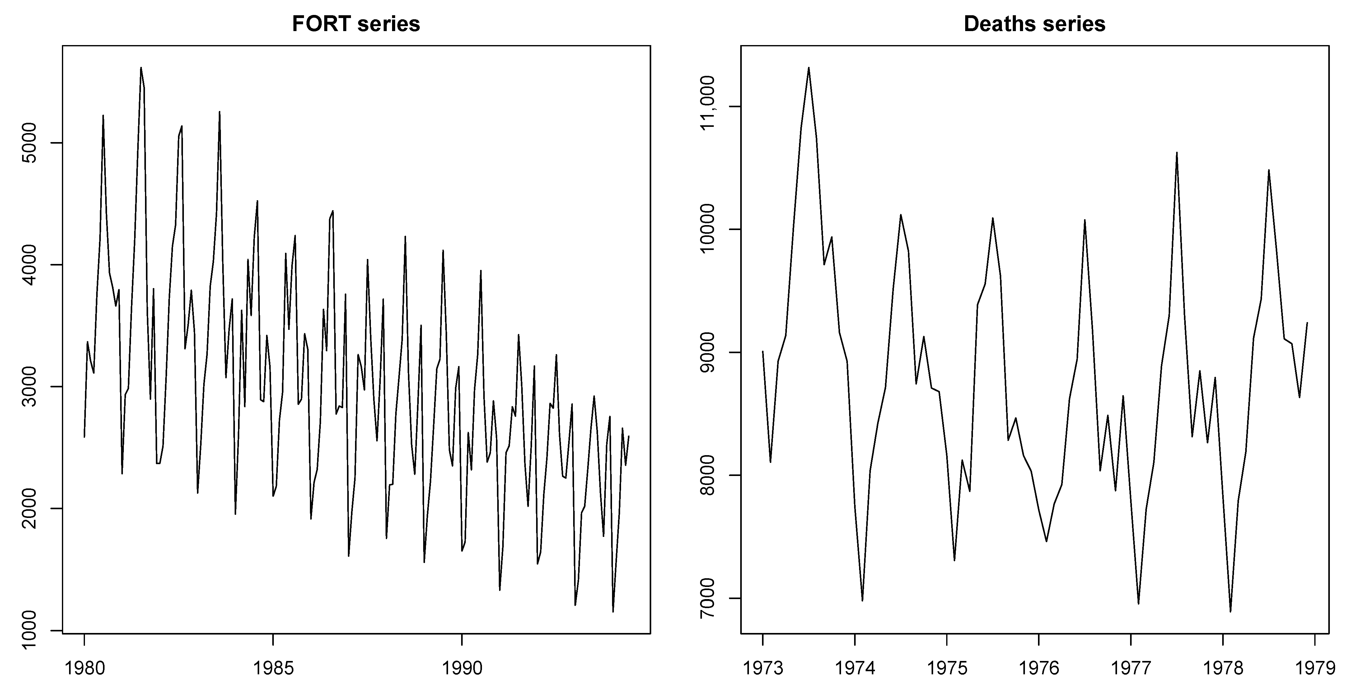
• FORT series: Monthly Australian fortified wine sales (abbreviated to “FORT”) in thousands of liters from January 1980 to July 1995 with 187 observations [14,31]. This time series is part of the dataset AustralianWine from R package Rssa. Each of the seven variables of the full dataset contains 187 points. Since the data were missing values after June 1994, we used the first 174 points.
• Deaths series: Monthly accidental deaths in the USA from 1973 to 1978 including a total of 72 observations. This well-known time series dataset has been used by many authors and can be found in many time series books (as can be seen, for example, [32]). In this study, the USAccDeaths data of R package datasets were used.

Figure 8 shows the time series plots of these datasets. It is evident that there is a seasonal structure in these time series. Furthermore, there is a downward linear trend in the FORT time series.

The following steps provide a simple step-by-step procedure to group the elementary components of the time series by means of a hierarchical clustering method:

Step 1: 

Choosing the window length

One of the most important parameters in SSA is the window length (L). This parameter plays a pivotal role in SSA because the outputs of reconstruction and forecasting are affected by changing this parameter. There are some general recommendations for the choice of the window length L. It should be sufficiently large and the most detailed decomposition is achieved when L is close to the half of time series length ($L\simeq N/2$) [10]. Furthermore, in order to extract the periodic components of a time series with the known period P, the window lengths divisible by the period P provide better separability [14].

In the FORT time series, which is periodic with the period $P=12$, $L=84$ meets these recommendations, since 84 is close to $\frac{N}{2}=\frac{174}{2}=87$ and $\frac{L}{P}=\frac{84}{12}=7$. Furthermore, the Deaths time series is periodic with the period $P=12$. Therefore, $L=36$ satisfies these recommendations, because 36 is equal to $\frac{N}{2}=\frac{72}{2}$ and $\frac{L}{P}=\frac{36}{12}=3$.

Step 2: 

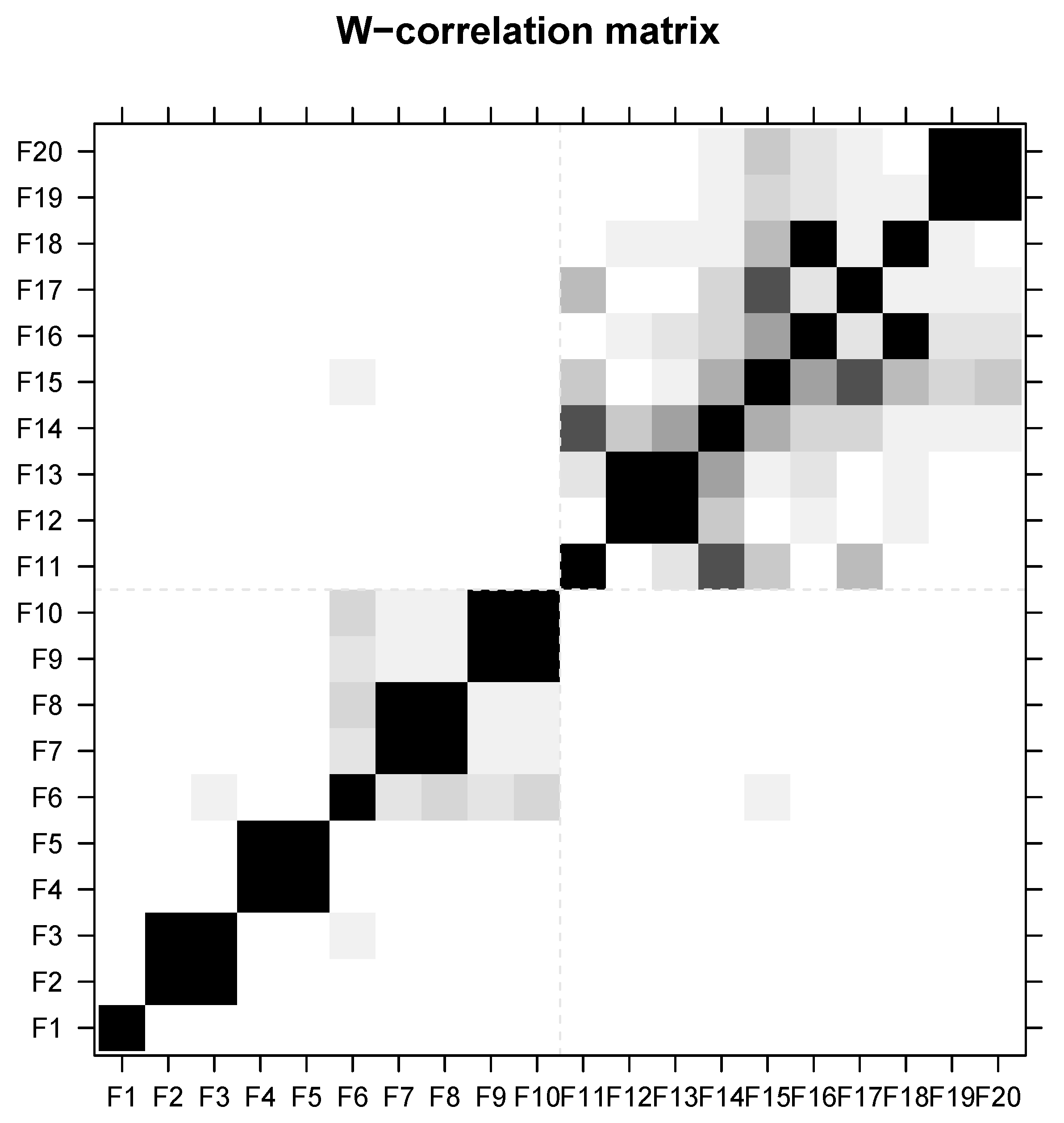
Determining the number of clusters

An important step in hierarchical clustering is the decision on where to cut the dendrogram. Similar to the simulation study proposed in Section 3, here, we use the number of clusters as a cutting rule of the dendrogram. If the purpose of time series analysis extracts the signal from noise, determining the number of clusters is quite straightforward; it is sufficient to set the number of clusters to equal two. However, if we want to retrieve different components concealed in a time series such as the trend and periodic components, determining the number of clusters requires more information. In this case, we recommend using the w-correlation matrix owing to utilizing it to measure the distance matrix of hierarchical clustering.

Figure 9 shows the matrix of absolute values of w-correlations between the 30 leading elementary reconstructed components of FORT series. The matrix of absolute values of w-correlations between the 36 elementary reconstructed components of Deaths series is depicted in Figure 10. In these figures, the white color corresponds to zero and the black color corresponds to the absolute values equal to one. Highly correlated elementary reconstructed components can be easily found by looking at the w-correlation matrix and then we can place these components into the same cluster.

It can be deduced from Figure 9 that the components of the FORT series can be partitioned into eight groups: $\left\{1\right\},\{2,3\},\{4,5\},\{6,7\},\{8,9\},\{10,11\},\{12,13\},\{14,\cdots ,84\}$. Furthermore, in order to separate signal from noise, the components can be split into two groups: signal ($\{1,\cdots ,13\}$) and noise ($\{14,\cdots ,84\}$).

Using the information provided in Figure 10, the components of Deaths series can be partitioned into seven groups: $\left\{1\right\},\{2,3\},\{4,5\},\left\{6\right\},\{7,8\},\{9,10\},\{11,\cdots ,36\}$. Additionally, in order to separate signal from noise, the components can be split into two groups: signal ($\{1,\cdots ,10\}$) and noise ($\{11,\cdots ,36\}$).

Step 3: 

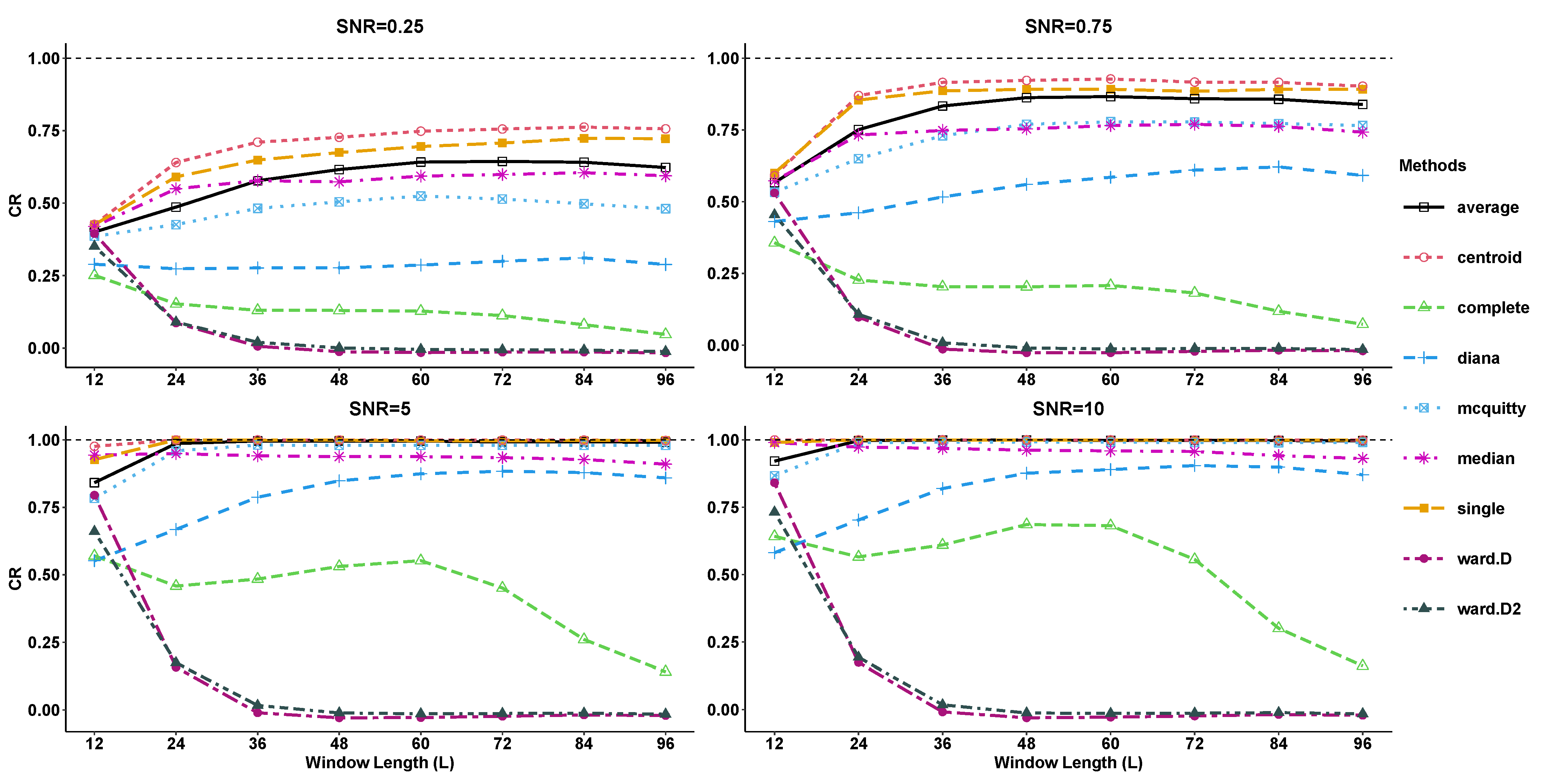
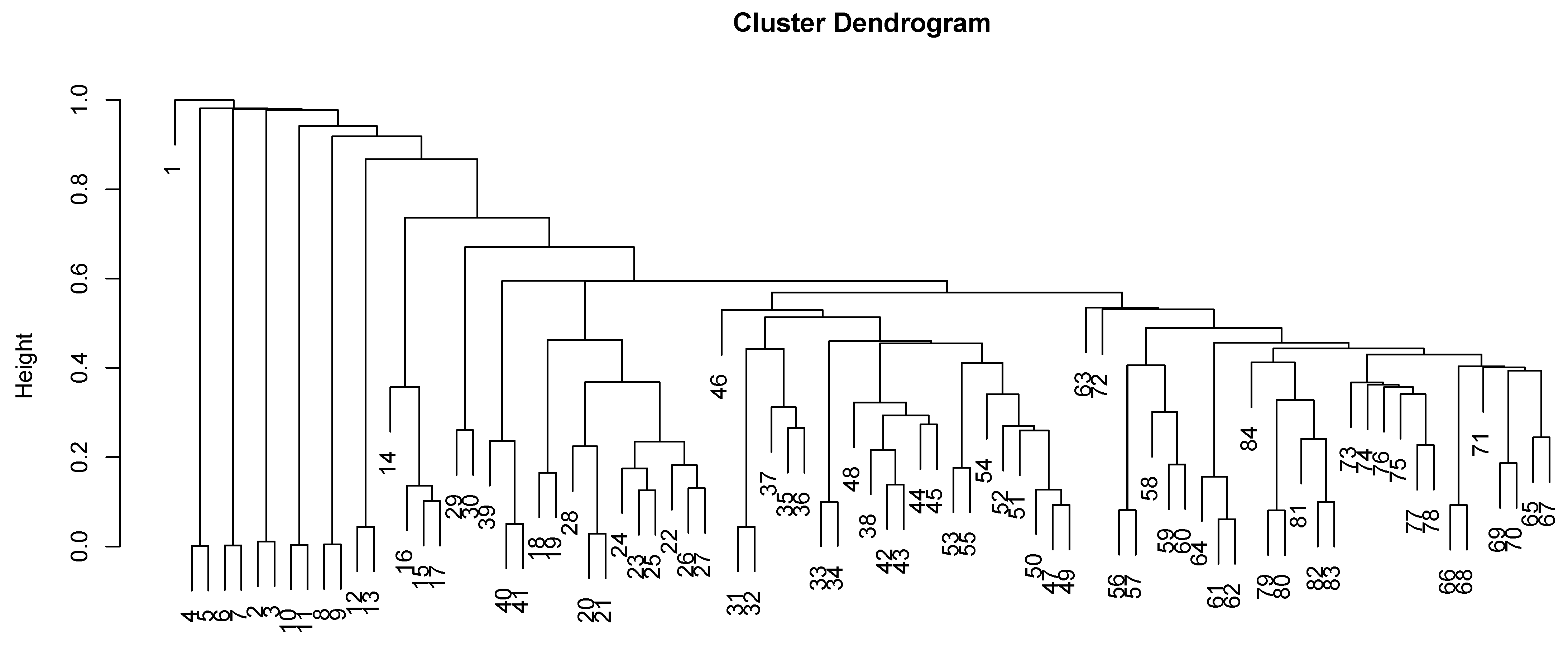
Selecting a proper linkage

Although a proper linkage can be selected using the findings of the simulation study given in Section 3, we compared the different linkages based on the CR index for FORT and Deaths series. The outputs of clustering are reported in

Table 4. Comparison of linkages for the FORT series.

Linkage	CR	Clustering Output
average	0.491	$\left\{1\right\},\{2,3\},\{4,5\},\{6,7\},\{8,9,12,13\},\{10,11\},\{14,\dots ,30\},\{31,\dots ,84\}$
centroid	1.000	$\left\{1\right\},\{2,3\},\{4,5\},\{6,7\},\{8,9\},\{10,11\},\{12,13\},\{14,\dots ,84\}$
complete	0.280	$\left\{1\right\},\{2,3\},\{4,\dots ,7\},\{8,9,12,13\},\{10,11,15,16,17\},$
		$\{14,18,\dots ,22,26,27,28,31,\dots ,60\},\{23,24,25,29,30\},\{61,\dots ,84\}$
diana	0.462	$\left\{1\right\},\{2,3\},\{4,5\},\{6,7\},\{8,9,12,13\},\{10,11\},$
		$\{14,\dots ,30,33,34\},\{31,32,35,\dots ,84\}$
mcquitty	0.491	$\left\{1\right\},\{2,3\},\{4,5\},\{6,7\},\{8,9,12,13\},\{10,11\},$
		$\{14,\dots ,30\},\{31,\dots ,84\}$
median	1.000	$\left\{1\right\},\{2,3\},\{4,5\},\{6,7\},\{8,9\},\{10,11\},\{12,13\},\{14,\dots ,84\}$
single	1.000	$\left\{1\right\},\{2,3\},\{4,5\},\{6,7\},\{8,9\},\{10,11\},\{12,13\},\{14,\dots ,84\}$
ward.D	0.028	$\{1,\dots ,13,29,30\},\{14,\dots ,17\},\{18,\dots ,28\},\{31,\dots ,45,48\}$
		$\{46,47,49,\dots ,55\},\{56,\dots ,64\},\{65,\dots ,71\},\{72,\dots ,84\}$
ward.D2	0.024	$\{1,\dots ,13,29,30\},\{14,\dots ,17\},\{18,\dots ,28\},\{31,\dots ,37,39,40,41,44,45,48\}$
		$\{38,42,43,47,49,\dots ,55\},\{46,63,65,\dots ,71\},\{56,\dots ,62,64\},\{72,\dots ,84\}$

and

Table 5. Comparison of linkages for the Deaths series.

Linkage	CR	Clustering Output
average	0.389	$\left\{1\right\},\{2,3\},\{4,5\},\{6,\dots ,10\},\{11,\dots ,18\},\{19,\dots ,30,32,33,34\},\{31,35,36\}$
centroid	1.000	$\left\{1\right\},\{2,3\},\{4,5\},\left\{6\right\},\{7,8\},\{9,10\},\{11,\dots ,36\}$
complete	0.158	$\left\{1\right\},\{2,3,11,14,15,17\},\{4,5,19,20,21,22,24\},\{6,\dots ,10\},\{12,13,16,18\},$
		$\{23,25,\dots ,34\},\{35,36\}$
diana	0.353	$\left\{1\right\},\{2,3\},\{4,5\},\{6,\dots ,10\},\{11,\cdots ,22\},\{23,\dots ,30\},$
		$\{32,33,34\},\{31,35,36\}$
mcquitty	0.389	$\left\{1\right\},\{2,3\},\{4,5\},\{6,\dots ,10\},\{11,\dots ,18\},\{19,\dots ,30\},$
		$\{32,33,34\},\{31,35,36\}$
median	0.761	$\left\{1\right\},\{2,3\},\{4,5,11,\dots ,30,32,\dots ,36\},\left\{6\right\},\{7,8\},\{9,10\},\left\{31\right\}$
single	0.914	$\left\{1\right\},\{2,3\},\{4,5\},\{6,7,8\},\{9,10\},\{11,\dots ,30,32,\dots ,36\},\left\{31\right\}$
ward.D	0.056	$\{1,6,\dots ,10,23,25,31,35,36\},\{2,3\},\{4,5\},\{11,\dots ,18\}$
		$\{19,\dots ,22\},\{24,26\dots ,30\},\{32,33,34\}$
ward.D2	0.111	$\{1,4,5,23,25,31,35,36\},\{2,3\},\{6,\dots ,10\},\{11,\dots ,18\}$
		$\{19,\dots ,24\},\{26,\dots ,30\},\{32,33,34\}$

, when it is assumed that the correct groups are those mentioned in Step 2. The results reported in these tables show that the single, median and centroid linkages can exactly identify the correct groups in FORT series (expressed in boldface). However, only the centroid linkage can exactly identify the correct groups in Deaths series (expressed in boldface). Based on the CR index reported in Table 4 and Table 5, it can be concluded that the ward.D and ward.D2 linkages have the worst performance both in FORT and Deaths series. These findings are in good agreement with the simulation results obtained in Section 3.

Figure 11 shows the dendrogram of the single linkage for our FORT series. The dendrogram of the centroid linkage for the Deaths series is depicted in Figure 12. The reconstruction of the FORT series with the help of the first 13 eigentriples is presented in Figure 13. Furthermore, Figure 14 shows the plot of the signal reconstruction of the Deaths series based on the first 10 eigentriples.

5. Conclusions

In this paper, we conducted a comparison study in order to find a proper hierarchical clustering method to identify the appropriate groups at the grouping step of SSA. In general, the simulation results provided a clear indication that the ward.D and ward.D2 linkages could not detect meaningful groups. In addition, the choice of the best hierarchical clustering linkage is not straightforward. It depends on the structure of a time series and the level of noise that disturbs a time series. In general, the evidence from this investigation suggests using the single, centroid, average and mcquitty linkages to group eigentriples in the grouping step of SSA.

It should be noted that our study has a clear limitation. It is due to the fact that in the automatic identification of SSA components, it should be assumed that the components to be identified are (approximately) separated from the rest of the time series.

References

- Atikur Rahman Khan, M.; Poskitt, D.S. Forecasting stochastic processes using singular spectrum analysis: Aspects of the theory and application. Int. J. Forecast. 2017, 33, 199–213. [Google Scholar] [CrossRef]
- Arteche, J.; Garcia-Enriquez, J. Singular Spectrum Analysis for signal extraction in Stochastic Volatility models. Econom. Stat. 2017, 1, 85–98. [Google Scholar] [CrossRef]
- Hassani, H.; Yeganegi, M.R.; Silva, E.S. A New Signal Processing Approach for Discrimination of EEG Recordings. Stats 2018, 1, 155–168. [Google Scholar] [CrossRef] [Green Version]
- Safi, S.M.; Mohammad Pooyan, M.; Nasrabadi, A.M. Improving the performance of the SSVEP-based BCI system using optimized singular spectrum analysis (OSSA). Biomed. Signal Process. Control. 2018, 46, 46–58. [Google Scholar] [CrossRef]
- Mahmoudvand, R.; Rodrigues, P.C. Predicting the Brexit Outcome Using Singular Spectrum Analysis. J. Comput. Stat. Model. 2018, 1, 9–15. [Google Scholar]
- Lahmiri, S. Minute-ahead stock price forecasting based on singular spectrum analysis and support vector regression. Appl. Math. Comput. 2018, 320, 444–451. [Google Scholar] [CrossRef]
- Saayman, A.; Klerk, J. Forecasting tourist arrivals using multivariate singular spectrum analysis. Tour. Econ. 2019, 25, 330–354. [Google Scholar] [CrossRef]
- Hassani, H.; Rua, A.; Silva, E.S.; Thomakos, D. Monthly forecasting of GDP with mixed-frequency multivariate singular spectrum analysis. Int. J. Forecast. 2019, 35, 1263–1272. [Google Scholar] [CrossRef] [Green Version]
- Poskitt, D.S. On Singular Spectrum Analysis and Stepwise Time Series Reconstruction. J. Time Ser. Anal. 2020, 41, 67–94. [Google Scholar] [CrossRef] [Green Version]
- Golyandina, N.; Nekrutkin, V.; Zhigljavsky, A. Analysis of Time Series Structure: SSA and Related Techniques; Chapman & Hall/CRC: Boca Raton, FL, USA, 2001. [Google Scholar]
- Golyandina, N.; Zhigljavsky, A. Singular Spectrum Analysis for Time Series, 2nd ed.; Springer Briefs in Statistics; Springer: Berlin/Heidelberg, Germany, 2020. [Google Scholar]
- Sanei, S.; Hassani, H. Singular Spectrum Analysis of Biomedical Signals; Taylor & Francis/CRC: Boca Raton, FL, USA, 2016. [Google Scholar]
- Hassani, H.; Mahmoudvand, R. Singular Spectrum Analysis Using R; Palgrave Pivot: London, UK, 2018. [Google Scholar]
- Golyandina, N.; Korobeynikov, A.; Zhigljavsky, A. Singular Spectrum Analysis with R; Springer: Berlin/Heidelberg, Germany, 2018. [Google Scholar]
- Golyandina, N. Particularities and commonalities of singular spectrum analysis as a method of time series analysis and signal processing. WIREs Comput. Stat. 2020, 12, e1487. [Google Scholar] [CrossRef]
- Bilancia, M.; Campobasso, F. Airborne particulate matter and adverse health events: Robust estimation of timescale effects. In Classification as a Tool for Research; Locarek-Junge, H., Weihs, C., Eds.; Springer: Berlin/Heidelberg, Germany, 2010; pp. 481–489. [Google Scholar]
- Korobeynikov, A. Computation- and space-efficient implementation of SSA. Stat. Its Interface 2010, 3, 257–368. [Google Scholar] [CrossRef] [Green Version]
- Golyandina, N.; Korobeynikov, A. Basic Singular Spectrum Analysis and forecasting with R. Comput. Stat. Data Anal. 2014, 71, 934–954. [Google Scholar] [CrossRef] [Green Version]
- Golyandina, N.; Korobeynikov, A.; Shlemov, A.; Usevich, K. Multivariate and 2D Extensions of Singular Spectrum Analysis with the Rssa Package. J. Stat. Softw. 2015, 67, 1–78. [Google Scholar] [CrossRef] [Green Version]
- Johnson, R.A.; Wichern, D.W. Applied Multivariate Statistical Analysis, 6th ed.; Pearson Education Ltd: London, UK, 2013. [Google Scholar]
- Kaufman, L.; Rousseeuw, P.J. Finding Groups in Data: An Introduction to Cluster Analysis; Wiley: New York, NY, USA, 1990. [Google Scholar]
- Maechler, M.; Rousseeuw, P.; Struyf, A.; Hubert, M.; Hornik, K. Cluster: Cluster Analysis Basics and Extensions. R Package Version 2021, 2, 56. [Google Scholar]
- R Core Team. R: A Language and Environment for Statistical Computing; R Foundation for Statistical Computing: Vienna, Austria, 2021; Available online: https://www.R-project.org/ (accessed on 23 October 2021).
- Charrad, M.; Ghazzali, N.; Boiteau, V.; Niknafs, A. NbClust: An R Package for Determining the Relevant Number of Clusters in a Data Set. J. Stat. Softw. 2014, 61, 1–36. [Google Scholar] [CrossRef] [Green Version]
- Gordon, A.D. Classification, 2nd ed.; Chapman & Hall: Boca Raton, FL, USA, 1999. [Google Scholar]
- Contreras, P.; Murtagh, F. Hierarchical Clustering. In Handbook of Cluster Analysis; Henning, C., Meila, M., Murtagh, F., Rocci, R., Eds.; Chapman & Hall/CRC: Boca Raton, FL, USA, 2016; pp. 103–123. [Google Scholar]
- Hennig, C.; fpc: Flexible Procedures for Clustering. R Package Version 2.2-9. 2020. Available online: https://CRAN.R-project.org/package=fpc. (accessed on 15 September 2021).
- Hubert, L.; Arabie, P. Comparing partitions. J. Classif. 1985, 2, 193–218. [Google Scholar] [CrossRef]
- Gates, A.J.; Ahn, Y.Y. The impact of random models on clustering similarity. J. Mach. Learn. Res. 2017, 18, 1–28. [Google Scholar]
- Vinh, N.X.; Epps, J.; Bailey, J. Information theoretic measures for clusterings comparison: Variants, properties, normalization and correction for chance. J. Mach. Learn. Res. 2010, 11, 2837–2854. [Google Scholar]
- Hyndman, R.J. Time Series Data Library. Available online: http://data.is/TSDLdemo (accessed on 10 May 2021).
- Brockwell, P.J.; Davis, R.A. Introduction to Time Series and Forecasting, 2nd ed.; Springer: Berlin/Heidelberg, Germany, 2002. [Google Scholar]