Stochastic Computing Implementation of Chaotic Systems

Abstract

An exploding demand for processing capabilities related to the emergence of the Internet of Things (IoT), Artificial Intelligence (AI), and big data, has led to the quest for increasingly efficient ways to expeditiously process the rapidly increasing amount of data. These ways include different approaches like improved devices capable of going further in the more Moore path but also new devices and architectures capable of going beyond Moore and getting more than Moore. Among the solutions being proposed, Stochastic Computing has positioned itself as a very reasonable alternative for low-power, low-area, low-speed, and adjustable precision calculations—four key-points beneficial to edge computing. On the other hand, chaotic circuits and systems appear to be an attractive solution for (low-power, green) secure data transmission in the frame of edge computing and IoT in general. Classical implementations of this class of circuits require intensive and precise calculations. This paper discusses the use of the Stochastic Computing (SC) framework for the implementation of nonlinear systems, showing that it can provide results comparable to those of classical integration, with much simpler hardware, paving the way for relevant applications.

1. Introduction

The increasing pervasion of devices related to wireless networks, data process, and transport and in general the Internet of Things (IoT) has led to a resultant rapid increase of edge devices. The numbers are enormous and the predictions are wondrous [1]; in five years (by 2025) 180 ZBytes will be the amount of data to be handled (International Data Corporation—IDC). In addition, IoT devices will exceed 150 billions and it is estimated that the data produced by them will be about 70% of the data produced worldwide (IDC) [1]. It is apparent that all the types of centralized processing, even in the form of cloud, cannot properly and efficiently support this new computing landscape, taking also into account the fact that IoT has to go hand in hand with other technologies regarding artificial intelligence, big data, mobile computing etc. which are being referred to as ubiquitous computing platforms. Therefore, edge computing rises in the horizon, calling for data processing at the edge of the network.

All these technologies call for innovative approaches [2,3] and some of those approaches are approximate computing [4,5,6], deep learning [7], new post-CMOS devices and architectures [8], or advanced processing techniques [9,10]. One of the fields where more computational power is required is communications, especially when data privacy protection and security are included. Thus, data encryption emerges as a mandatory element. Nowadays, many techniques and approaches are proposed in the context of the IoT, in all hierarchical levels of data communications, others for ensuring privacy [11] and others for practically ensuring security [12]. As a result, there exist numerous proposals in this sense, usually ubiquitous ones; one such promising option seems to lean towards using chaotic-based encoder-decoder schemes to secure and/or authenticate data transmission in general [13,14,15,16]. There are examples of such secure-communication systems, analog [17,18], and digital [19,20] ones demonstrating merits like low-cost, circuit simplicity, low-power operation etc. [9,10,21,22].

On the other hand, it seems that approximate computing enables high power savings [6], making this technique a viable candidate for IoT edge devices. This framework offers energy savings by trading accuracy for energy. There are a handful of methods that can successfully implement approximate computing: programming methods and algorithms, hardware implementations, and other ubiquitous solutions. As a curious side note, this strongly reminds one of the way chaos was encountered by Lorenz, finding different solutions of his equations because of truncated number storage [23]. In fact, as the legend goes, Lorenz found that saving the state of a simulation and using it as the new initial condition, resulted in a very different simulation than simply continuing this without saving. After a lot of analysis effort, it was found that results were stored with less resolution than was used internally to perform the computations. This difference in the number of bits caused minuscule differences that led to divergent simulations because of the chaotic nature of the system. Thus, it is quite important to analyze if the system to be implemented allows the use of approximate computing.

An interesting approach had been already introduced by Von Neumann in 1956 [24], based on a series of lectures given by R.S. Pierce in 1952 at California Institute of Technology. This approach, namely Stochastic Computing (SC) or Stochastic Logic, makes a trade off between calculation time and accuracy. This approach has been successfully applied in fields as diverse as neural network implementation [25,26], data mining [27], data compression [28], or mathematical calculations (FFT) [29], control [30], or even A/D conversion [31], among others. Indicative of its advantages, it allows for a high reduction in the number of components, thus reducing the power required to run the circuit. However, this comes to a price, since the time required to perform the operation also increases exponentially with the number of bits. This, in turn, may increase the total energy consumption when the number of bits exceeds 16–17 [32,33]. There are, however, techniques that allow this problem to be alleviated, and make this competitive even for higher bit-numbers [33]. Notice, that stochasticity is entering only in the proper (for calculation) number generation and has nothing to do with the systems implemented within this framework. In fact, it could be considered as an equivalent of typical noisy system.

There are cases where this trade-off plays a crucial role, like in the case of chaotic systems. It is known that key features of all nonlinear, chaotic systems are: long-term bounded aperiodic behavior, enhanced sensitivity to parameters and initial conditions, and fast decorrelation between past and present [34]. These features, especially sensitivity to initial conditions and parameter values, make proper implementation of chaotic systems within approximate computing frameworks, difficult, not impossible though. A successful example is the case of implementing a chaotic oscillator in a purely digital environment [20] but with the cost of creating a much more complicated (higher-dimensional) implementation.

In this paper, having in focus possible utilization of chaotic systems for edge computing applications, like the IoT, an unconventional approach to the computation of nonlinear dynamical systems, is investigated. Specifically, we show how the stochastic computing (SC) framework, an option for approximate computing, can be utilized to properly implement nonlinear, chaotic operating systems. It is apparent that approximate computing methods for implementing systems sensitive to initial conditions and system parameters is an important issue that needs thorough investigation. In Section 2 an introduction to Stochastic Computing is apposed, presenting some very basic examples; Section 3 presents a method in the form of an example, on how to implement a nonlinear system using both this framework and a classical integration, as well. Then, established nonlinear dynamics tools and metrics like fractal dimension, Kolmogorov-Sinai entropy etc. are utilized to estimate how well the described SC implementation behaves, compared to the conventional approach. Finally, Section 4 concludes the paper.

2. Stochastic Computing Implementation of Analog Systems

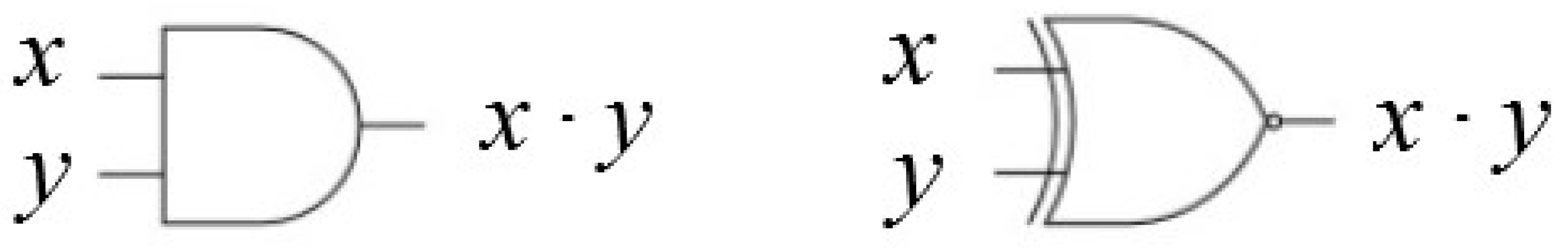
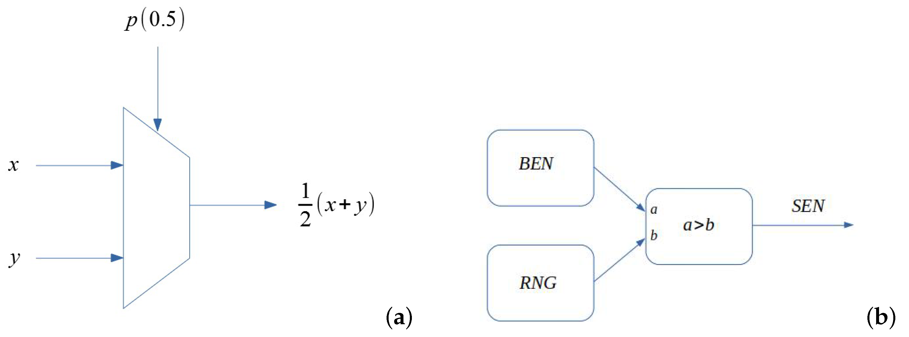
2.1. Introduction to Stochastic Computing

The SC approach means representing real numbers by a string of random binary numbers. The average value of this string (between zero and one) is correlated to the number represented [35]. These strings are called Stochastic Computing numbers (SCN) or Stochastic Encoded Numbers (SEN). In this paper, we will opt for the second, using also the term Binary Encoded Numbers (BEN) for those encoded as classical binary numbers. There are two main mappings from real to SEN: one from the real domain [0,1], and another one from the real domain [−1,1].

Depending on the chosen mapping, several operations can then be carried out with different simple logic gates. In the case of the real [0,1] domain, multiplication of Stochastic Computing numbers is calculated using an AND gate. In the case of the [−1,1] domain, multiplication requires the use of an XNOR gate, as shown in Figure 1.

The case of addition is slightly more complex, since 1 + 1 = 2, and we cannot represent any number as a probability higher than one. Thus, the operation that should be implemented is $(x+y)/2$, which will always be 1 at the most. This operation is usually implemented using a multiplexer, as shown in Figure 2a, where the p (0.5) means a signal with a probability of 0.5 to be “1” or “0”. This signal is generated using one of the bits generated in the RNG, so no additional circuitry is needed. It is worth pointing out that this gate is the same both for the [0,1] and the [−1,1] domains. Other more complex operations (division [30], square roots [30], reversible gates [36], etc.) are also discussed in the literature, though they are not to be presented here to focus on the implementation procedure of the non-linear equation system.

Another important point is the conversion from BEN to SEN. This is usually achieved by using a scheme similar to that in Figure 2b, where an N-bit random number is generated by utilizing a random number generator (RNG) and compared to the value of the N-bit BEN. If the output of the RNG is below the BEN, the converter’s output would be a 1-bit “1”, or a 1-bit “0” otherwise. In the opposite operation, converting SEN back to its BEN representation, the number of 1’s included in the signal needs to be calculated; something that can be achieved by a simple counter.

It is apparent that the error in the approximation of the SEN to its actual value is equivalent to the error provided by a random walk process of length n, and thus proportional to $\sqrt{n}$, as it has been discussed in the literature [37]. Therefore, using N bits, we may consider that all the noise caused by the process is included in the lowest $N/2$ bits. This way, the noise figure $NF$ for a signal of power $S_p$ with noise power $N_p$ caused by the use of the $SCN$ is:

$$NF=10lo{g}_{10}\left(\frac{S_p}{N_p}\right)=10lo{g}_{10}\left(\frac{2^N}{2^{N/2}}\right)\approx 3.01N/2\mathrm{dB}$$

(1)

Notice that for this equation we have considered the maximum possible amplitude for the input signal. In order to consider the minimum amplitude $\mathrm{over}$ the noise, we consider we are 1 bit over the noise ($N/2+1$). In this case, we obtain:

$$NF=10lo{g}_{10}\left(\frac{S_p}{N_p}\right)=10lo{g}_{10}\left(\frac{2^{N/2+1}}{2^{N/2}}\right)\approx 3.01\mathrm{dB}$$

(2)

Thus, the system is expected to have a NF between 3 dB and $3\left(N/2+1\right)$ dB, assuming as above that we use more than 1 bit. This $NF$ sets the required number of bits, which is related to the sensitivity of the equation system to noise. Empirically, we have seen that linear equations allow for a low N, while nonlinear systems call for higher values. Notice that a value of the $NF=20$ dB calls for N = 12 bits, while N = 32 bits would provide $NF=54$ dB.

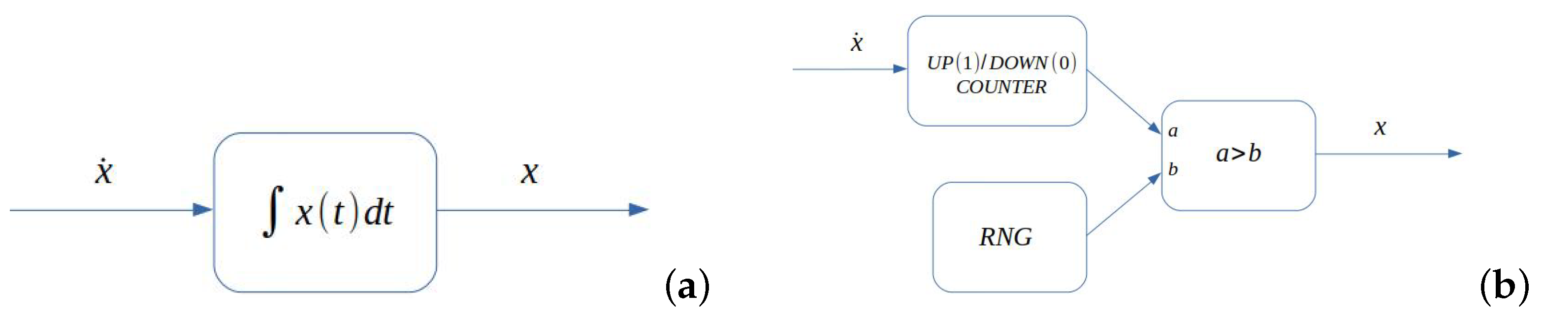
2.2. Implementation of Basic Differential Equations

Implementation of differential equations using SC is similar to the case of implementing them in discrete form. The process involves, mainly, rewriting the equation in a specific way so they can be integrated using SC. This requires three different transformations:

• Rewriting the equation in a form suited to SC. In the most basic case, this implies replacing all the additions by half additions: $a+b\to 2(a/2+b/2)$. Other, more complex operations may require a harder reworking of the equations to ensure all the operations can be implemented in SC in the [−1,1] or [0,1] range. For instance, in the case of implementing a division, one has to ensure that the result is always going to be in range, which may require an additional scaling and shifting of the variables involved.
• Scaling all the variables into the [−1,1] or [0,1] domains, since those are the values that can be dealt with in SC.
• Then, a final transformation ensures that all the modules of the coefficients in the equations are lower than 1. This is equivalent to a time scaling.

Once these three transformations are performed, the equations may be processed as a SC system. It is apparent that in this procedure multiplications are implemented by the gates appearing in Figure 1 and additions by the half-additions implemented by the gate in Figure 2a.

In order to implement the integrator the scheme appearing in Figure 3 is utilized. This figure shows the symbol to be used in Figure 3a, while the scheme is shown in Figure 3b. It performs a continuous integration, by counting up or down depending on whether the input is 1 or 0 and comparing the output of the counter with a random number generator RNG to create a $SCN$. The implementation of the integrator and the RNG implies making a decision on the effective number of bits demanded in order to define the size of the counter. Notice that this is equivalent to determining the precision of the integrator, since numbers are represented between [0,1] (or [−1,1]) with N bits of resolution and a noise figure provided by Equation (1). Related to the number of RNG needed to implement this scheme, it has been shown in [38] that using the same RNG in both inputs actually improves the accuracy, thus simplifying the design.

Related to this number of bits is the issue of way time is mapped to the number of iterations, in the relevant SC equations. This is an issue strongly dependent on the integration method; assuming that a simple first order rectangular integration, with no explicit time dependence is utilized, then, it is apparent that the following Equation (3) holds valid:

$$\begin{array}{cc}\hfill \dot{x}& =f\left(x\right)\hfill \\ \hfill \dot{x}& \approx \frac{\Delta x}{\Delta t}=f\left(x\right)\to \Delta x=f\left(x\right)\Delta t\hfill \end{array}$$

(3)

Using the integrator scheme presented in Figure 3, we see that allowing for a high enough number of $N_{acc}$ iterations, the output at the counter $Int\left(x\right(t\left)\right)$ would be:

$$\begin{array}{c}\hfill Int\left(x\right)=\frac{N_{acc}·p\left(1\right)}{2^N}\end{array}$$

(4)

where $p\left(1\right)$ is the probability of having a 1 at the input. It has to be noted that $p\left(1\right)$ corresponds to the actual value to be represented in the SCN, and $N_{acc}$ is the number of “ones” the accumulator has counted. Thus, equating Equation (3) with Equation (4), we find that the effective time step is given in Equation (5).

$$\Delta t=\frac{N_{acc}}{2^N}$$

(5)

Notice that the integrator depicted in Figure 3 also includes a binary to stochastic (B2S) converter, which is simply a random number generator (RNG), plus a comparator. This way, the output of the integrator is already also a SC number that can be used further in the circuit.

2.3. Basic Examples

As a proof of concept two basic examples are presented: a system that integrates twice a constant and a simple oscillator. We have implemented these systems into a DE2-70 Field Programmable Gate Array (FPGA) by Altera, using Quartus-II to compile it. The resulting circuits were implemented using less than 500 gates or less than a 2% of the available number of gates. Communication with the computer was implemented using the JTAG interface, controlled within Matlab.

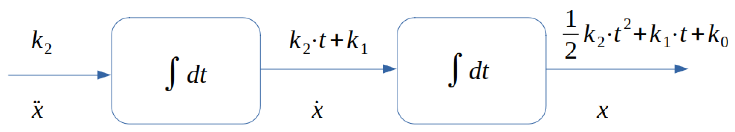
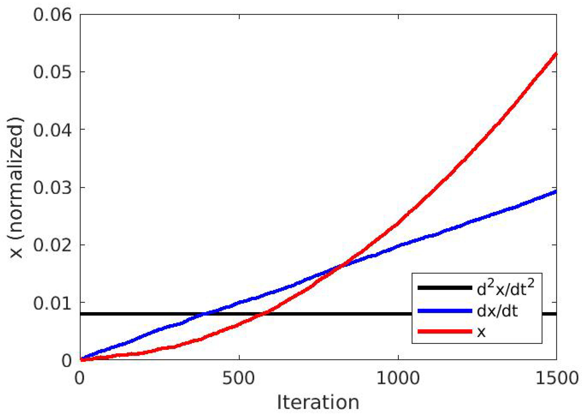
2.3.1. Integrating a Constant (Twice)

As a first example, we have designed the system shown in Figure 4 and Equation (6) and initial conditions ($\ddot{x},\dot{x},x) = (k_2,k_1,k_0$). The system then integrates the equations over time.

$$\begin{array}{ccc}\hfill \dot{x}& =y\hfill & \hfill (x(t=0)=k_0)\\ \hfill \dot{y}& =z\hfill & \hfill (y(t=0)=k_1)\\ \hfill \dot{z}& =0\hfill & \hfill (z(t=0)=k_2)\end{array}$$

(6)

The analytical solution of the system above, is provided in Figure 4 and the results for a specific set of initial conditions are depicted in Figure 5 (for initial conditions $k_0=k_1=0$, and $k_2=0.08$). In this figure, we have used $N_{acc}=5000$ iterations and $N=21$ bits, resulting in a time-step $\Delta t=\frac{5000}{2^{21}}\approx 2.384\mathrm{ms}$. Using this relation, we expect the line corresponding to $\dot{x}$ reaching $\ddot{x}\left(k_2\right)$ at the 420th iteration and crossing the parabola generated by x at the 839th iteration. The parabola is expected to cross $k_2$ at iteration 593. Actually, all these crossings emerged exactly at the expected points, as shown in Figure 5.

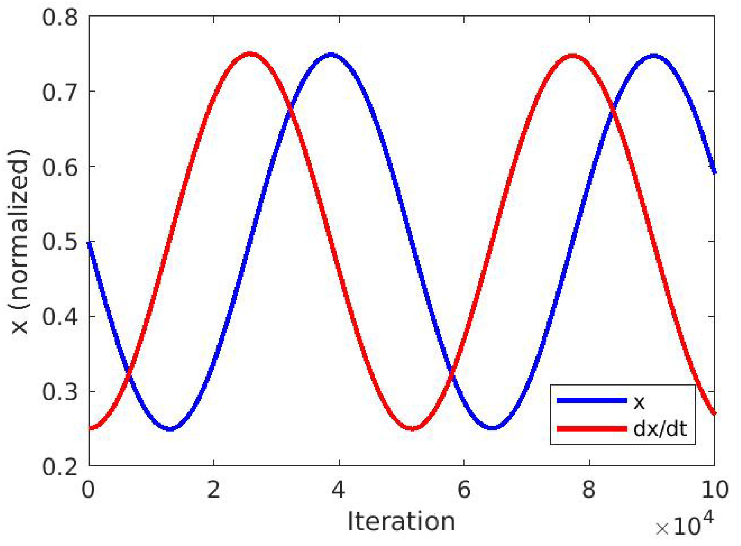
2.3.2. A Simple Oscillator

The simplest possible autonomous system to be implemented was that of a self-oscillating system; this is a simple coupled system described in Equation (7) implementing a simple oscillator of frequency one ($\omega =1$), corresponding to the system illustrated in Figure 6.

$$\begin{array}{cc}\hfill \dot{x}& =y\hfill \\ \hfill \dot{y}& =-x\hfill \end{array}$$

(7)

In this case, the implementation is direct, by simply replacing the blocks in Figure 6, with those discussed above. The resulting waveforms of both x and y variables are shown in Figure 7. In this figure, we have used $N_{acc}=2^4=16$ iterations and $N=18$ bits. This provides a $\Delta t=\frac{2^4}{2^{18}}=\frac{1}{8192}\mathrm{s}$. Using this relation, the period is expected to be $2\pi /\Delta t\approx$ 51,497 iterations, as it actually happens in Figure 7.

3. Implementing Chaotic Systems in SC

Implementation of chaotic systems using stochastic computing can be achieved by using the same three step process presented above. The main issue in this case regards the sensitivity to noise, for such systems. Thus, an adequate NF will require a high number of bits. To compare the results coming from integrating within the proposed SC environment, to those utilizing the conventional methods, the Shimizu-Morioka system [39] was utilized as a paradigm. Therefore, a comparison between these two implementations of some typical nonlinear time series analysis estimators (Kolmogorov entropy, correlation dimension, etc.) were performed; documenting an evaluation of the effectiveness of the SC implementation. It should be mentioned that the classical integration was performed using Matlab, while the $SCN$ was performed using the same FPGA as in the previous section.

Regarding the RNG, we have used a single 64-bit implementation of the Mersenne algorithm, which provides a period long enough for our purposes. Notice that most of the RNG we need are only 1-bit long, so we can extract all of them from the same RNG. In addition, we have used the technique proposed in [40], which allows for the use of a single generator to create different random numbers to the integrators and constants to the generators. The scaling constants are stored as fixed registers, which are then used to generate the random sequence through a B2S converter. It is worth noticing that the RNG is actually responsible of a large part of the total energy consumption, due to the large number of computations needed by the algorithm. This energy consumption could be addressed in the future by using memristors to generate the random bits, as proposed in [41,42,43].

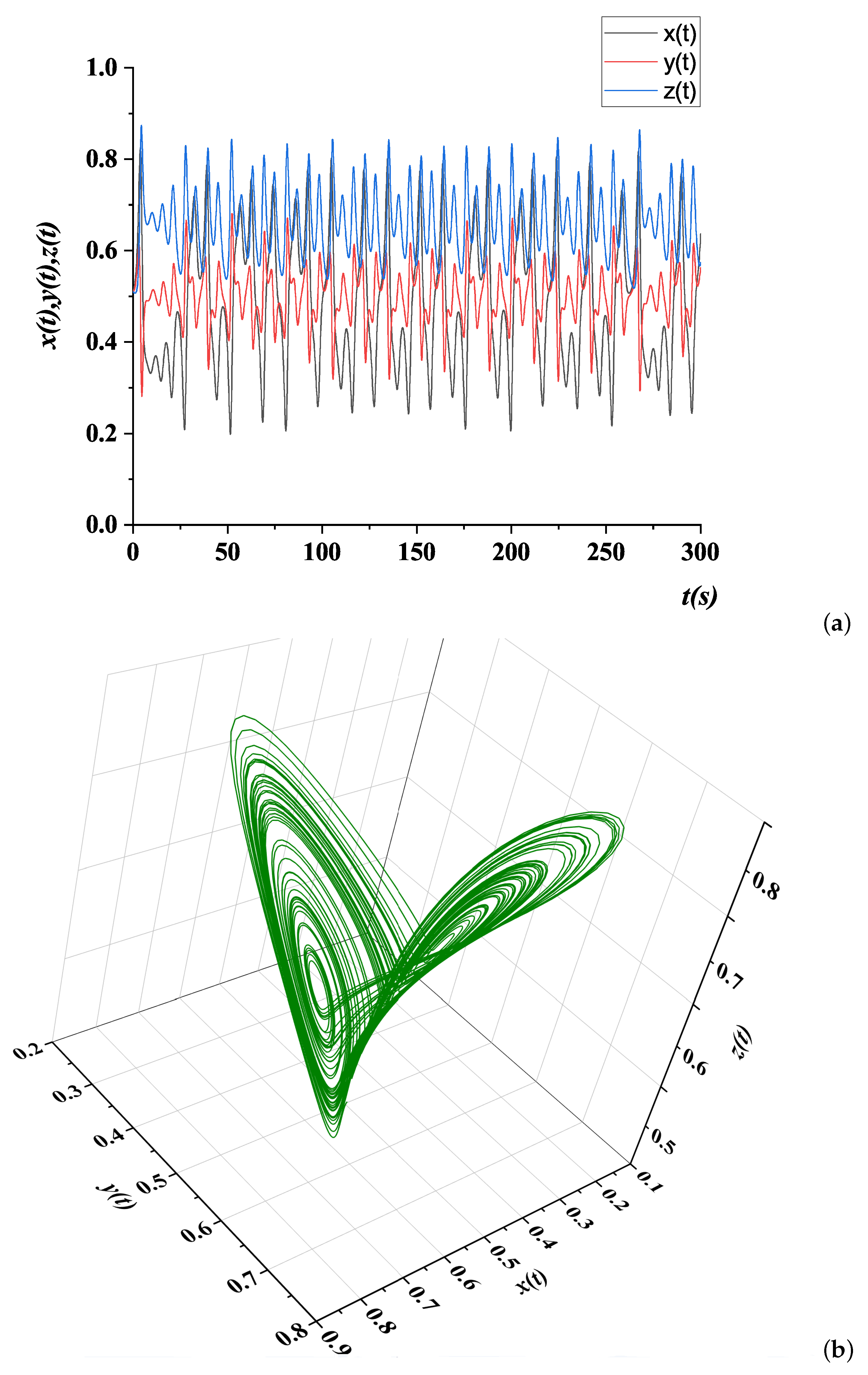
3.1. The Shimizu-Morioka System

A system algebraically simpler than the Lorenz system has been proposed by Shimizu and Morioka [39] in 1980. The original equation formulation appears below:

$$\left.\begin{array}{cc}\hfill \dot{x}& =y\hfill \\ \hfill \dot{y}& =x-\mu ·y-x·z\hfill \\ \hfill \dot{z}& =-\alpha ·z-x^2\hfill \end{array}\right\}\mathrm{Shimizu}\mathrm{Morioka}\mathrm{System}$$

(8)

A usual set of parameter values, leading to the emergence of chaos in this system, is $\mu =0.81$ and $\alpha =0.375$. By applying this set, the system is operating in a deterministic chaotic mode, demonstrating an elegant chaotic attractor in the corresponding 3D phase space. As expected for deterministic chaotic systems, the trajectories comprising this strange attractor are bounded, while the whole system behavior appears to be bounded within a box (the phase space), the limits of which are explicitly presented in relations (9).

$$\left.\begin{array}{c}\hfill xϵ(-1.5,1.5)\\ \hfill yϵ(-1,1)\\ \hfill zϵ(-2.5,2.5)\end{array}\right\}\mathrm{Variable}\mathrm{Boundaries}$$

(9)

3.2. Equation Preparation

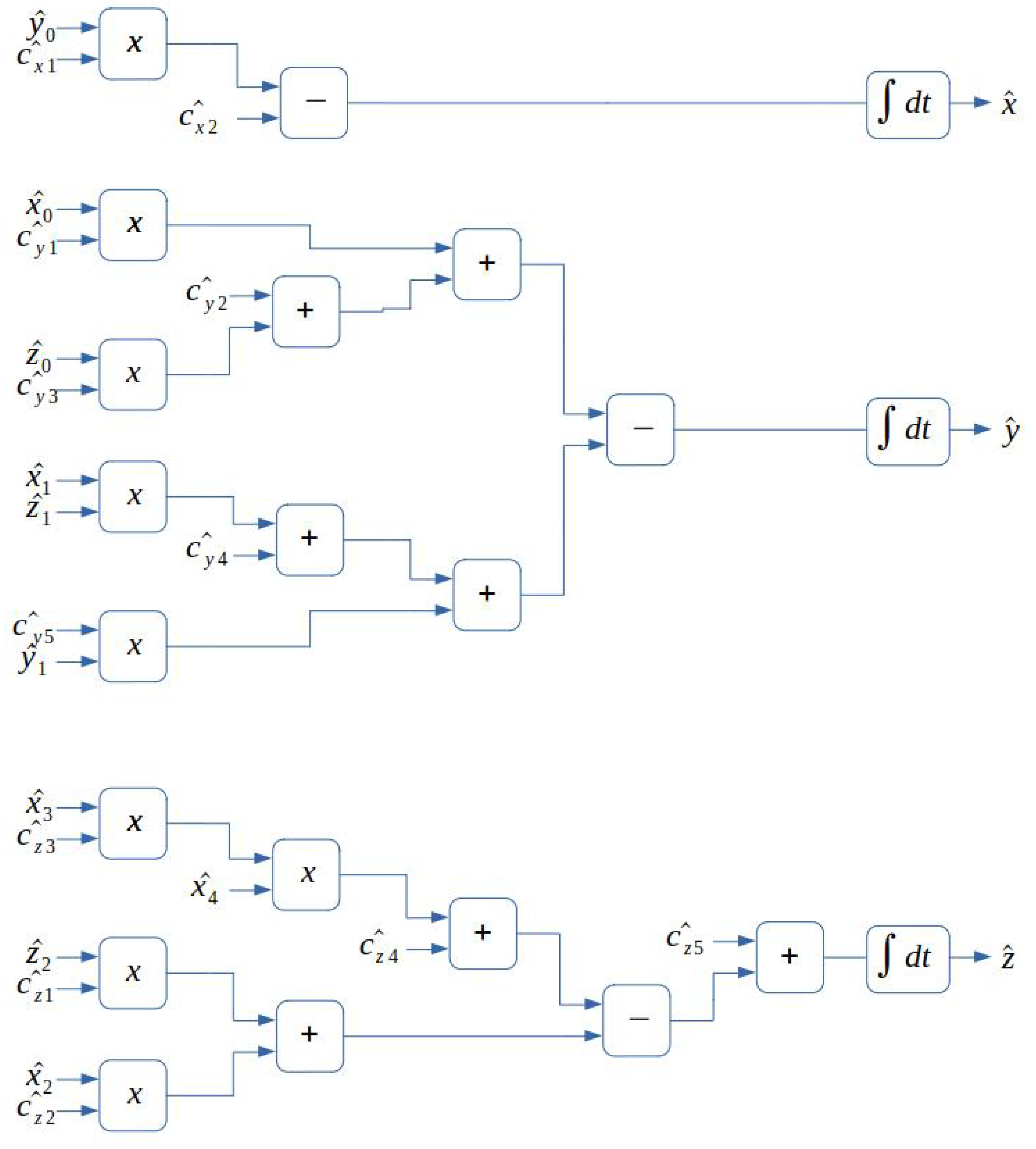
It is apparent that the next step in implementing equation set (8) in SC environment, is to get through a normalization procedure, as this has been discussed above. This would ensure that all three variables ($x,y,z$) would be within the SC working interval. In our case, we opted for normalizing all the variables to be within the [0,1] range. In order to achieve this, the following variable transform (10) was applied, as a first step:

$$\left.\begin{array}{c}\hfill X=-\frac{x+2}{4}\to x=4X-2\\ \hfill Y=-\frac{y+2}{4}\to y=4Y-2\\ \hfill Z=-\frac{z+3}{6}\to z=6Z-3\end{array}\right\}$$

(10)

It is apparent that the proposed change of variables transformed equation set (8) into the form appearing in equation set (12), after getting through the relations in (11).

$$\left.\begin{array}{c}\hfill \dot{x}=4\dot{X}=y\\ \hfill \dot{y}=4\dot{Y}=x-\mu y-xz\\ \hfill \dot{z}=6\dot{Z}=-\alpha z+x^2\end{array}\right\}$$

(11)

$$\left.\begin{array}{c}\hfill \dot{X}=Y-\frac{1}{2}\\ \hfill \dot{Y}=4X-2+\frac{1}{2}\mu -\mu Y+3Z-6XZ\\ \hfill \dot{Z}=-\alpha Z+\frac{\alpha }{2}+\frac{8}{3}{X}^2+\frac{2}{3}+\frac{8}{3}X\end{array}\right\}$$

(12)

Thus, the resulting equation system in (12) has all its ($X,Y,Z$) variables oscillating within the proper range for stochastic logic, but the equations are not yet ready to be implemented in a SC environment. This is due to the fact that some of the system-parameters are outside the SC range (in this case higher than one). To solve this, we divided all the terms by a number $c_r$ higher than the highest coefficient appearing in the equations. Notice that this is equivalent to a scaling of time of a magnitude $t^{\prime }=c_{r}t$, thus no qualitative change emerges. In this specific case, using the value $c_r=32$, the equation set (12) became as follows:

$$\left.\begin{array}{cc}\hfill \dot{X}& =\frac{Y}{32}-\frac{1}{64}\hfill \\ \hfill \dot{Y}& =\frac{X}{8}-\frac{1}{16}+\frac{\mu }{64}+\frac{3Z}{32}-\frac{3XZ}{16}-\frac{\mu Y}{32}\hfill \\ \hfill \dot{Z}& =-\frac{2X}{24}-\frac{\alpha Z}{32}+\frac{\alpha }{64}+\frac{2X^2}{24}+\frac{1}{48}\hfill \end{array}\right\}$$

(13)

However, it has to be noted that, even if all the parameters and variables are within the proper range, the operations are not in a form ensuring that their results would fall within the SC range. In specific, the additions must be in the form suggested in Equation (14).

$$a+b=\frac{1}{2}\left(2a+2b\right)$$

(14)

Rewriting all the equations according to this requirement, the equation set (13) transforms into in the one appearing in (15), which is the final form of the equations to be implemented in the SC environment.

$$\left.\begin{array}{cc}\hfill \dot{X}& =\frac{1}{2}(\frac{Y}{16}-\frac{1}{32})\hfill \\ \hfill \dot{Y}& =\frac{1}{2}\left[\frac{1}{2}[\frac{1}{2}(X-\frac{1}{2})+\frac{1}{2}(\frac{\mu }{8}+\frac{3Z}{4}]]-\frac{1}{2}-\frac{1}{2}(\frac{3XZ}{4}+\frac{\mu Y}{8})\right]\hfill \\ \hfill \dot{Z}& =\frac{1}{2}\left[\frac{1}{2}\left[-\frac{1}{2}\left(\frac{2X}{3}+\frac{\alpha Z}{4}\right)+\frac{1}{2}\left[\frac{\alpha }{8}+\frac{2X^2}{3}\right]\right]+\frac{1}{24}\right]\hfill \end{array}\right\}$$

(15)

3.3. Implementation

The equation set (15) was implemented in a Matlab environment, being integrated in a conventional way by utilizing its built-in functions and the ode45 solver with variable time step. The solution of the system for all three system-variables in the time domain appears in Figure 8a for specific initial conditions. In Figure 8b the corresponding attractor of the system, in its 3-dimensional phase space, is apposed.

The same system (beginning from the same initial conditions) has also been implemented in a SC environment using the previously discussed basic gates and it is presented in Figure 9. In this figure, the $x_i$ variable corresponds to any of the signals x, delayed by i clock cycles, an essential approach that improves decorrelation. Note that the delay element is not shown, but it is simply implemented by a shift register, taking into account that the variables are only 1 bit long. The number of bits used in this implementation was $N=22$, with $N_{acc}=2^{12}$ iterations. This would be equivalent to a conventional system using 17-bit binary arithmetic, once the noise has been taken into account.

The results corresponding to this integration are presented in the form of time series (in the time-domain) in Figure 10a, where all three variables $X,Y,Z$ appear. The corresponding attractor, embedded in a 3D phase space, appears in Figure 10b. Comparing these two figures to the corresponding Figure 8a,b of the classical implementation, one gets the subjective perception that the two implementations evolve in time in a quite similar way, not the same though. Indeed, although in both implementations the systems begin evolving in time from the same initial conditions, their evolution is not identical, due to the approximate computing approach implemented in SC environment. However, the emerging attractors are in both cases demonstrating almost identical structure in their embedding phase space (3D in this case). A very draft remark is that the time series and the resulting attractor appears to be slightly more noisy, in the case of SC implementation, something expected because of the approximate nature of calculations in the case of SL.

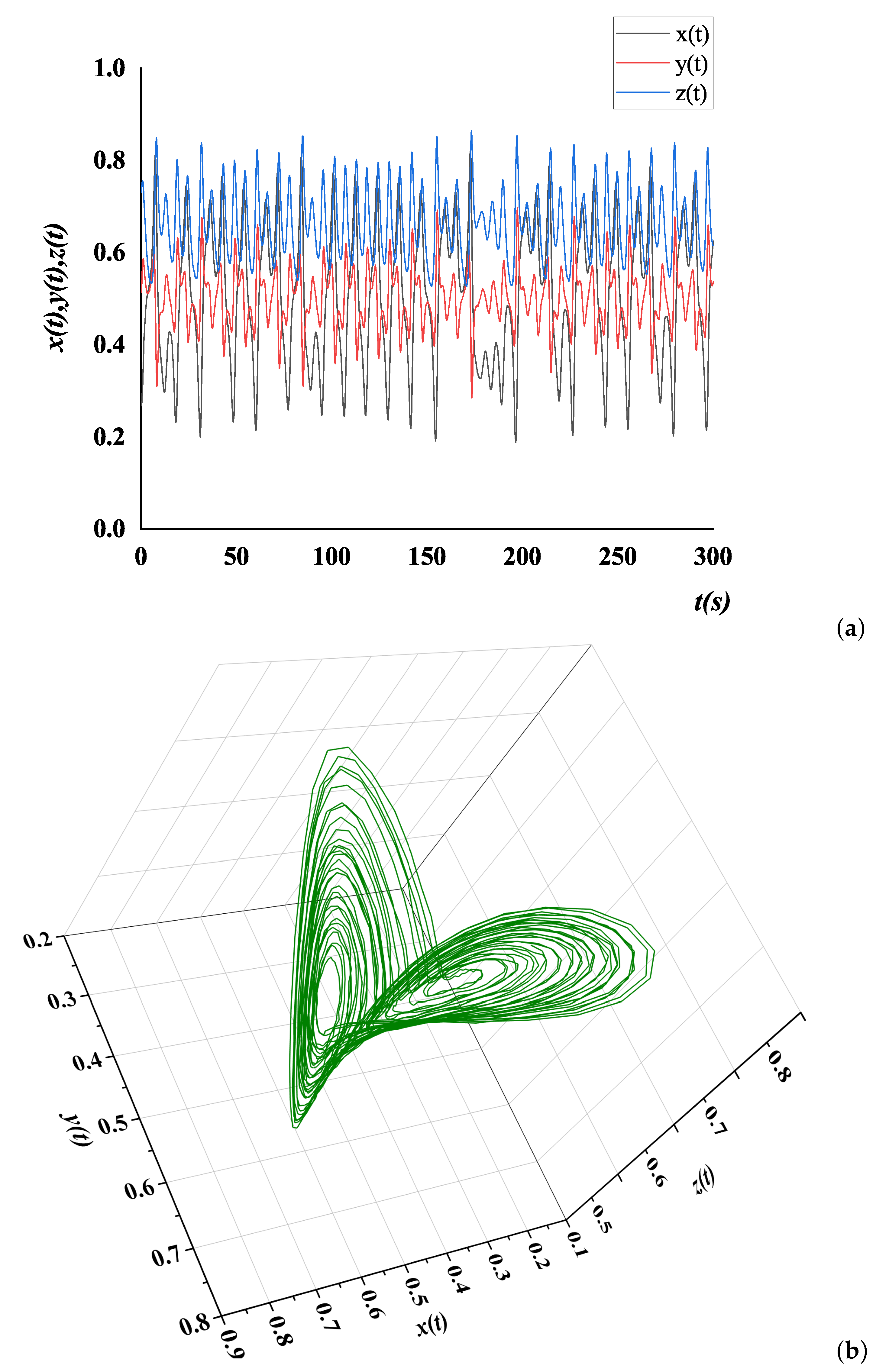
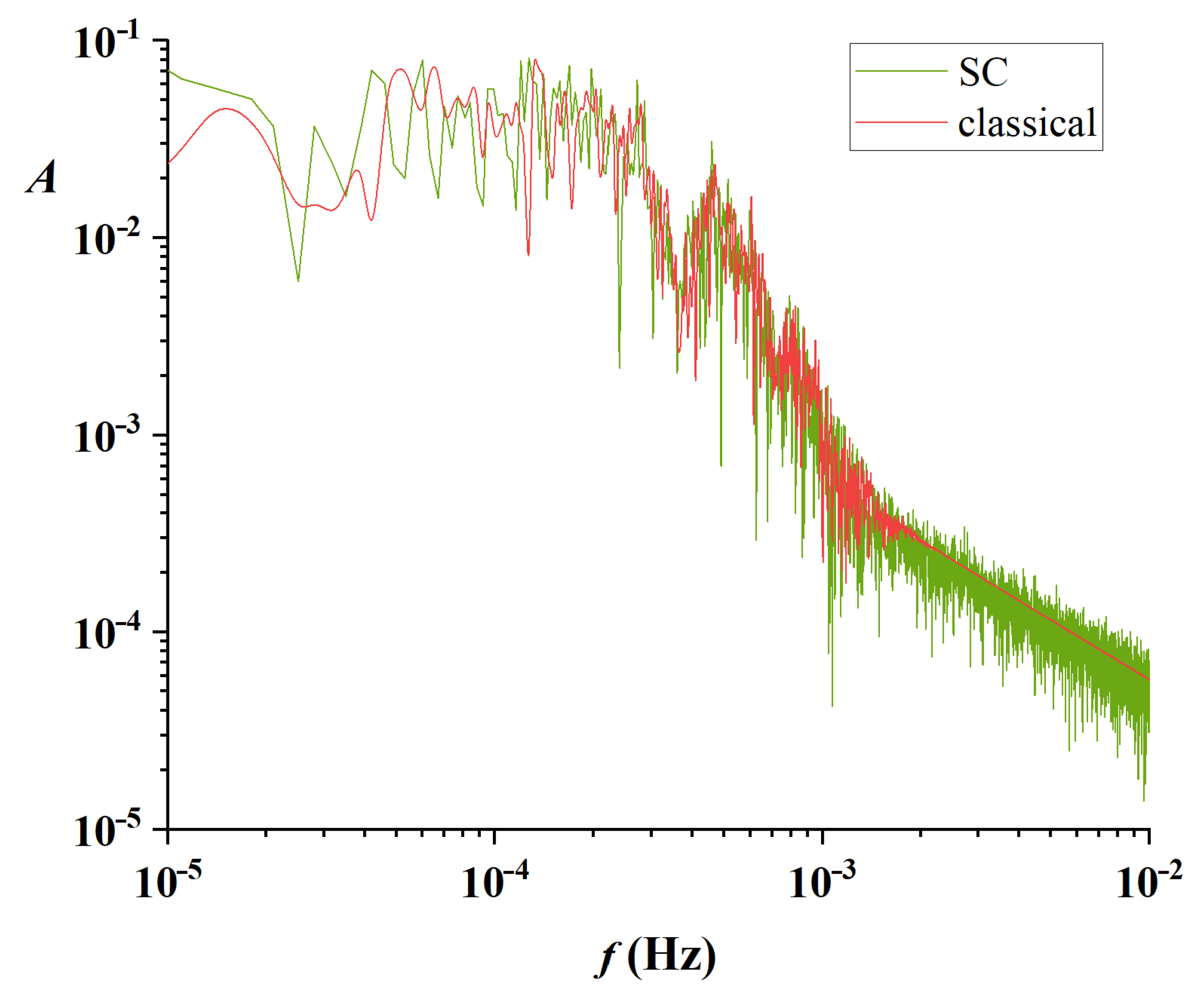
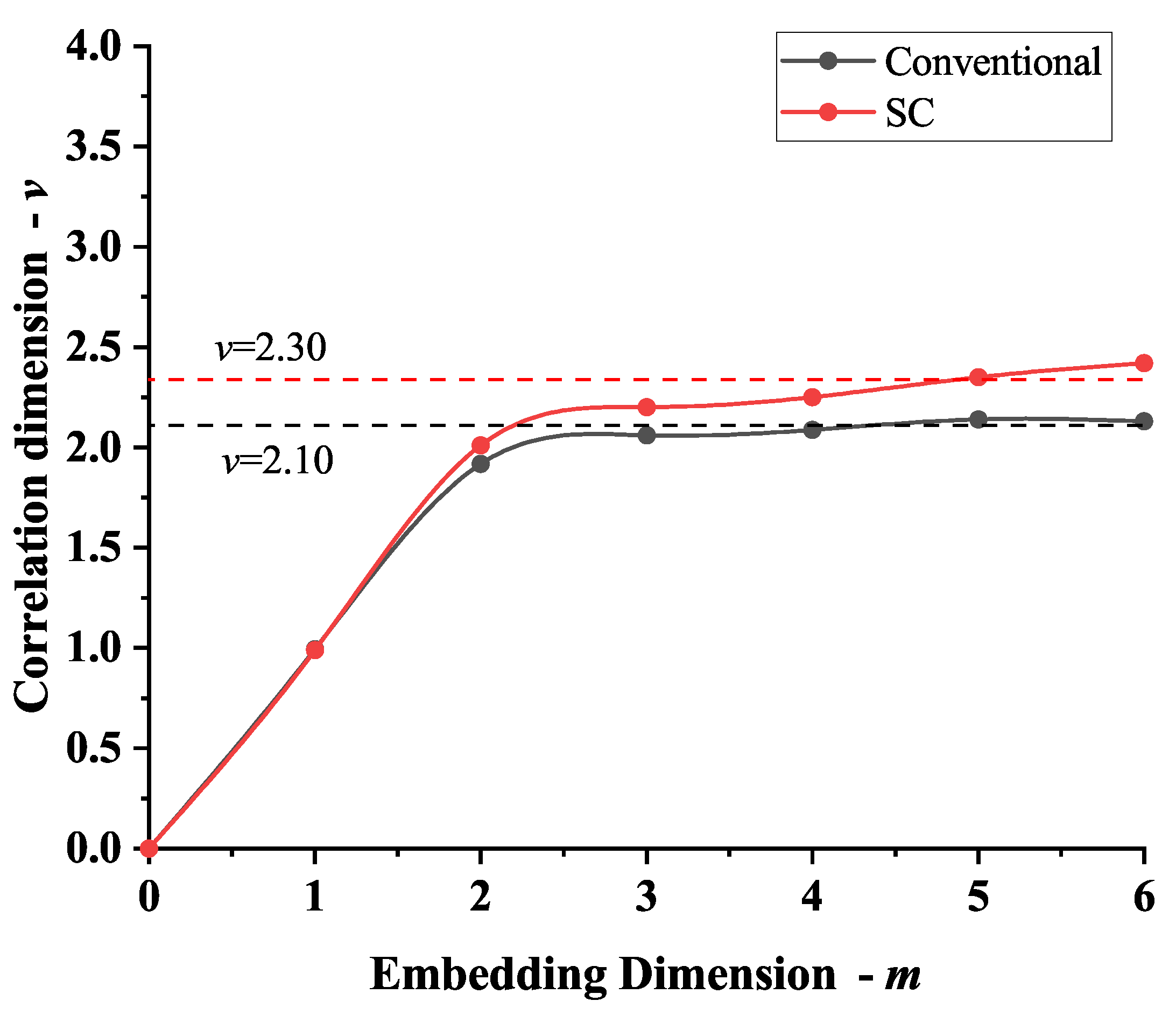
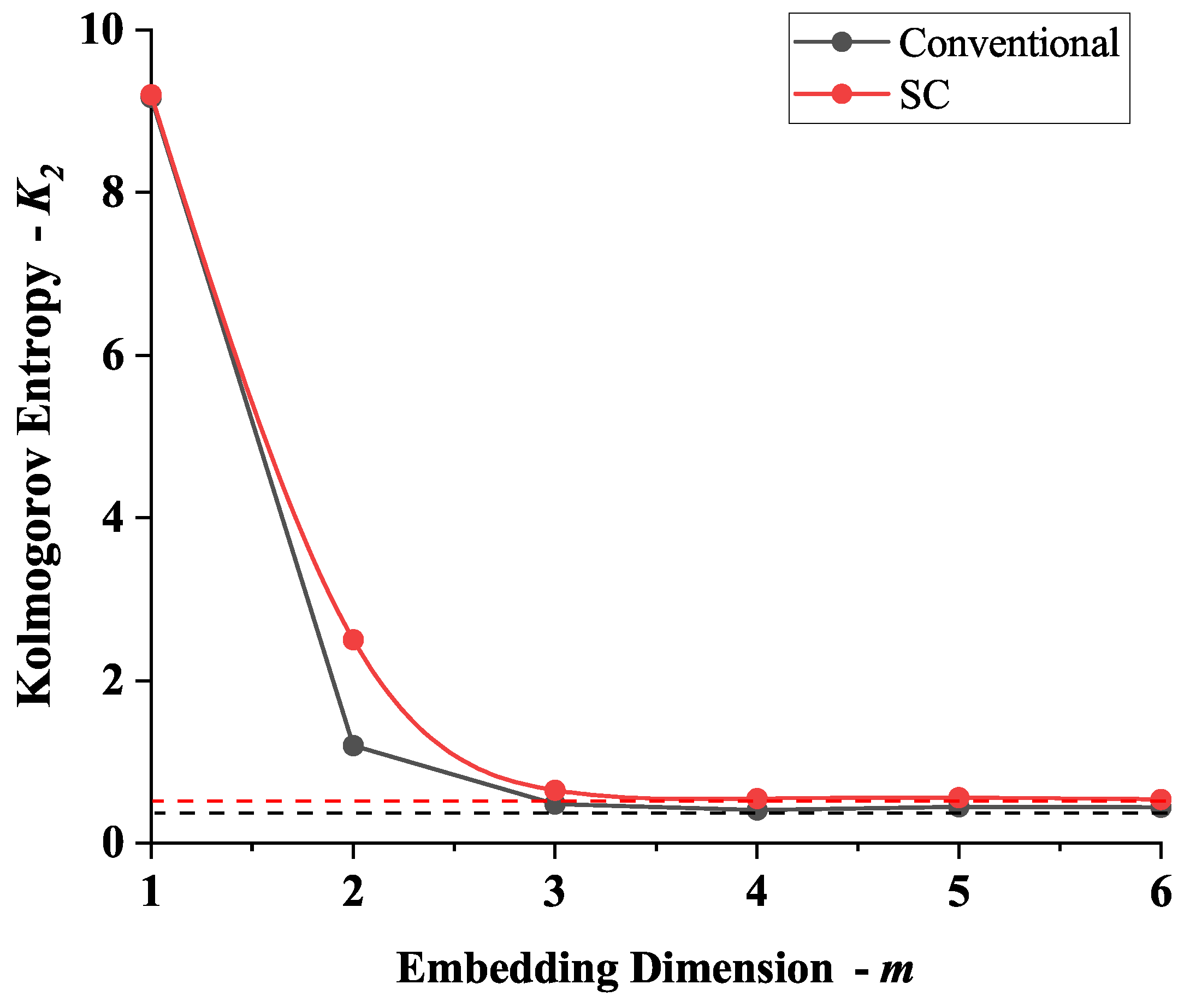
3.4. Chaotic Evaluation

Due to the nature of deterministic chaotic systems and in order to perform a more objective investigation of the fidelity of the dynamics demonstrated by the Shimizu-Morioka equation system, in the stochastic computing environment, a procedure including a variety of relevant metrics was applied.

Initially, the power spectrum of one of the state variables, namely $Z\left(t\right)$, was calculated in both cases. It is presented in Figure 11, where the red line regards the classical integration method and the green line the SC method. The similarity between them is obvious, including the minimum at around 0.35 mHz and the maximum at 0.5 mHz. The most apparent difference appears in the higher frequencies, which can be attributed to both the error in number quantization [44] and the noise from a random walk [37] as expressed in Equations (1) and (2).

Further investigation and analysis of the demonstrated chaotic behavior included calculation of correlation dimension, Kolmogorov entropy, as well as Lyapunov exponents. To this direction, the $z\left(t\right)$ and $Z\left(t\right)$ variable from the three time series appearing in Figure 8a and Figure 10a correspondingly, were considered.

Applying the Takens theory [45] to the $Z\left(t\right)$ time series, the topologically equivalent attractor was reconstructed, in the proper phase space. It is noted that according to this theory, the technique of displaced vectors is applied. So initially, the appropriate time delay $\tau$, needed for the reconstruction of the phase space, was calculated by both the mutual information’s first local minimum and the autocorrelation function’s first zero. In both cases, the conventional and the SC solution, the value emerging for $\tau$ appeared to have a significantly lower value when calculated through the mutual information, and therefore this was the one adopted [23]; for the specific set of parameters and initial conditions: $\tau$ = 16 for the conventionally calculated solution and $\tau$ = 8 for the SC solution (in both cases we refer to measurement points).

The correlation integrals $C(2,\ell )$, for different embedding dimensions, have been numerically calculated, according to the Grassberger-Procaccia method [46,47,48], Equation (16):

$$C_m(2,\ell )=\sum p_i^2=\underset{N\to \infty }{lim}\frac{1}{N^2}\sum _{\begin{array}{c}\mathrm{i},\mathrm{j}=1\\ \mathrm{i}\ne \mathrm{j}\end{array}}^N\Theta \left(\ell -\sqrt{\sum _{k=1}^m{\left|X_{j+k}-X_{i+k}\right|}^2}\right)$$

(16)

where parameter ℓ is the hypercube dimension in the hyperphase space for a series of specific embedding dimensions m, and $\Theta$ the Heaviside function. These integrals provided information characterizing the attractor and were calculated for embedding dimension up to $m=6$, for both the conventional and the SC solutions of $Z\left(t\right)$. In both cases, the integrals appeared to almost parallelize for embedding dimensions $m=3$ and above. The slopes of the correlation integrals’ linear parts (in a double logarithmic scaling) were determined for each embedding dimension (v vs. m) and their values appear in Figure 12. In this plot, the black line refers to conventional solution, while the red one to SC. In both cases a saturation plateau appears for $m\ge 3$, thus, this is the sufficient phase space dimension, necessary to host the system’s global dynamics under any circumstances [23].

In the case of the conventional solution (black line in Figure 12), the saturation tends to the noninteger value of $v=2.10$, which is the correlation dimension of the attractor under these circumstances, further proving the deterministic chaotic nature of the studied time series (and the corresponding system). The closest (to the correlation dimension) higher, integer value defines the minimum embedding dimension, which in this case appears to be $m_{min}=3$, as expected for a three state-variable system. It is apparent that for the Shimizu Morioka system, the calculated minimum embedding dimension coincides with the minimum sufficient phase space dimension $m_{min}=m_{suff}=3$.

In the case of the SC solution (red line in Figure 12) the relation of the correlation integral slope, for all the embedding dimensions (v vs. m) is again saturated after $m=3$, but this time to a slightly higher noninteger value; thus the correlation dimension in this case is $v=2.30$. This difference is something expected and fully explainable, since the approximate computing nature of SC is introducing a specific level of noise, which is expected (and hereby verified) to increase the attractor’s dimensionality. However, this increase is within the system’s minimum dimensions $m_{min}=m_{suff}=3$.

In order to investigate the global chaotic dynamics, the Kolmogorov-Sinai Entropy and the Lyapunov exponents were calculated. The Kolmogorov Entropy appears in Figure 13, in both cases. It clearly possesses positive value, $K_2=0.44$ bits/$\tau$ for the conventional solution, and $K_2=0.54$ bits/$\tau$ for the SC solution. These values are almost the same depicting similar rate of loss of information of the past state of the system; therefore, there is a similar deterministic chaotic nature for both implementations.

Finally, the three (as expected for a three-dimensional system) corresponding average local Lyapunov exponents, as they were calculated by the observed $Z\left(t\right)$ time series [49], are presented in

Table 1. Values of the first three Lyapunov exponents for the “Z” variable in the cases of classical integration and SC integration.

Order	Classical	SC
${\lambda }_1$	0.02112	0.03774
${\lambda }_2$	−0.00487	−0.00462
${\lambda }_3$	−0.31142	−0.29139

. The maximal exponent provides with a measure of the predictability of system producing the studied time series [49,50]. If at least one of them is positive then the system is chaotic. In both investigated cases, the system demonstrates one positive exponent, one nearly zero (due to the finite time series and the approximation introduced by the calculating method) and one negative, hinting for a simple chaotic system. Moreover, in both implementations the values were close one to the other. The higher value of ${\lambda }_1$ in the case of the SC solutions, is again expected and due to the noise introduced by the approximate calculations taking place in the case of the SC implementation [23,34]. Additionally, the second exponent ${\lambda }_2$ is zero in both cases as expected, and the third ones ${\lambda }_3$ are also close in value. It is noted that in this case the value of the maximal exponent (the only positive) also provides the lower bound of the Kolmogorov-Sinai entropy.

All the above calculations of nonlinear dynamics established metrics prove and confirm the ability to implement the chaotic dynamics of Shimizu-Morioka system in SC, indifferent to the approximate nature of this kind of calculations.

4. Discussion

Having in focus edge computing and data trafficking in the frame of the IoT, approximate computing emerges as an essential technological option, being able to provide low cost in both area and energy for (relatively) low precision calculations. To this direction, in this work we have presented a detailed procedure to implement nonlinear equations using stochastic computing (a kind of an approximate computing method). This procedure involves a renormalization of the equations in three phases: first, it sets the possible values of the variables inside the values [−1,1]; secondly, all the constants inside the equations are recalculated so that they would also lay within the same range, which is equivalent to a scaling of the time variable; finally, all the operations are rewritten in a form compatible to the available operations in stochastic computing.

We have also discussed the effect of changing the number of bits used to represent the variables, showing that this number is related to the signal-to-noise ratio that the system can withstand. Specifically, since the process is a random walk, the noise figure is expected to grow according to the bit-string length, as $\sqrt{N}$.

The main advantage of the presented approach is the low number of components needed to implement the equations, which is far below the required number demanded in the classical approach, due to the method of implementing SC calculations. This makes the specific approach useful for small (lightweight) systems that require making complex calculations with a low energy consumption, mainly if the needed number of bits is not large. In addition, the robustness of nonlinear systems in the frame of SC was also shown. This is specially relevant, since nonlinear systems are highly sensitive to initial conditions and parameter variations, which may greatly change their long-term behavior. In our case, we have shown that this long-term behavior is kept, even when all the constants and parameters have been defined as $SCN$.

As examples of application, we have implemented three different systems representing as many differential equation systems: a double integrator, a simple oscillator, and a nonlinear system. As already discussed above, the results from the first two cases appear to be exactly the same as the conventional system implementations. In the case of the Shimizu-Morioka system, which has been used as the toy model for nonlinear system implementation, the results obtained using SC are consistent with a conventional implementation. The metrics used for comparing the implementation in the SC versus the conventional one were three: the correlation dimension (2.10 for the conventional case, 2.30 for the SC); the Kolmogorov entropy (0.44 bits/$\tau$ for the conventional, 0.54 bits/$\tau$ for the SC); and the Lyapunov exponents, which were also found to be very similar.

Related to the performance of the system in stochastic computing; it is clear that its worse aspect is the time needed to perform the calculations. In the proposed FPGA implementation, the throughput of the system is one bit per clock cycle, and it needs 2${}^N$ cycles to perform a single $\delta t$ iteration. This total time can be reduced by parallelization. Thus, using M identical blocks in parallel as proposed in [33], the total time needed to perform the iteration is reduced accordingly to be $t_{SC}=$2${}^N$/M clock cycles. On the other hand, when considering conventional binary operations implemented sequentially, the total time would be given by:

$$t_{conv}=\sum _x{N}_x{\tau }_x$$

(17)

where ${\tau }_x$ is the number of cycles needed to implement the arithmetic operation x, which appears $N_x$ times in the circuit. In our case, we only have used multiplication (mul), addition (add), subtraction (sub), and integration (int). Of those, multiplication needs usually between 3 and 7 clock cycles, and the others only 1, since the integral is just another addition. Thus, for our system, we need a total of clock cycles between 40 and 76, with an expected value around 67 cycles. Thus, for a 16 bit implementation with M parallel SC branches, the ratio between $t_{conv}$ and $t_{SC}$ is:

$$\frac{t_{conv}}{t_{SC}}=M\frac{{\sum }_x{N}_x{\tau }_x}{2^N}=M\frac{67}{65536}\approx M/1000$$

(18)

Thus, for a simple implementation with 32 parallel branches, the conventional arithmetic would be 32 times faster than a Stochastic Computing equivalent. This, as has been discussed above, leads to a trade-off between speed, precision, and power consumption. Notice, however, that for an application requiring a lower number of bits (as, for instance, in [51], where only 10 bits are needed), this is changed to ≈M/16 and an SC implementation could be actually faster and simpler than a conventional one.

Related to the other performance parameters of the system, we have to note that in this paper we are focusing only on the possibility of implementing such systems, with no emphasis on the energy consumption or area optimization. These two aspects are still under consideration for our proposal, since the literature seems to be unclear in this aspect. However, as an example, related to the area optimization, we can compare the difference between the number of logic elements needed to implement a stochastic computing (always a simple gate) against a usual digital implementation of a vedic multiplication [52] into a certain FPGA, as in [53]. These results are compiled in

Table 2. Comparison of the number of Field Programmable Gate Array (FPGA) parts used for implementation of the vedic multiplication algorithm [53] and the SC multiplication. (*) The number of LUTs used in SC is considered to be 1/3 of a 6-input LUT, as those in the FPGA used in [53].

Algorithm	bits	Slices	LUTs
Vedic	4	19	33
SC	6	1	1/3 *
Vedic	16	346	622
SC	22	1	1/3 *
Vedic	32	1427	2566
SC	32	1	1/3 *

and show a clear advantage of SC over conventional implementation. Related to energy consumption, it is known [33] that for short bit-streams (less than 16–17 bits) SC performs better than conventional. Notice, in any case, that the energy consumption needed to generate the random bits is not taken into account, since they can be generated in multiple ways. For instance, a 64-bit Mersenne RNG needs a lot of power to perform all the calculations that lead to the pseudorandom sequence of bits, but if we can use memristors for this task [41,42,43] this energy is drastically reduced, as well as the needed area. Additionally, a final ASIC implementation of the design could utilize some improvements, as extensively discussed in [33], that allow for exponential improvement of consumption.

The results emerging from the SC implementation are thus showing that this technique is capable of implementing complex nonlinear systems, in an area-efficient way, with small loss of precision, equivalent to an analog circuit implementation. Taking into account their possible application for secure data transmission, they are one possible alternative to be considered in IoT, or Edge computing systems, paving the way for an even wider spread of IoT.

References

1. Shi, W.; Pallis, G.; Xu, Z. Edge Computing [Scanning the Issue]. Proc. IEEE 2019, 107, 1474–1481. [Google Scholar] [CrossRef]
2. Venkataramani, S.; Roy, K.; Raghunathan, A. Efficient embedded learning for IoT devices. In Proceedings of the 2016 21st Asia and South Pacific Design Automation Conference (ASP-DAC), IEEE, Macau, China, 25–28 January 2016; pp. 308–311. [Google Scholar]
3. Shafique, M.; Theocharides, T.; Bouganis, C.S.; Hanif, M.A.; Khalid, F.; Hafız, R.; Rehman, S. An overview of next-generation architectures for machine learning: Roadmap, opportunities and challenges in the IOT era. In Proceedings of the 2018 Design, Automation & Test in Europe Conference & Exhibition (DATE), IEEE, Dresden, Germany, 19–23 March 2018; pp. 827–832. [Google Scholar]
4. Xu, Q.; Mytkowicz, T.; Kim, N.S. Approximate computing: A survey. IEEE Des. Test 2015, 33, 8–22. [Google Scholar] [CrossRef]
5. Jayakumar, H.; Raha, A.; Kim, Y.; Sutar, S.; Lee, W.S.; Raghunathan, V. Energy-efficient system design for IoT devices. In Proceedings of the 2016 21st Asia and South Pacific Design Automation Conference (ASP-DAC), IEEE, Macau, China, 25–28 January 2016; pp. 298–301. [Google Scholar]
6. Gao, M.; Wang, Q.; Arafin, M.T.; Lyu, Y.; Qu, G. Approximate computing for low power and security in the internet of things. Computer 2017, 50, 27–34. [Google Scholar] [CrossRef]
7. Du, L.; Du, Y.; Li, Y.; Su, J.; Kuan, Y.C.; Liu, C.C.; Chang, M.C.F. A reconfigurable streaming deep convolutional neural network accelerator for Internet of Things. IEEE Trans. Circuits Syst. I 2017, 65, 198–208. [Google Scholar] [CrossRef] [Green Version]
8. Ipek, E. Memristive Accelerators for Dense and Sparse Linear Algebra: From Machine Learning to High-Performance Scientific Computing. IEEE Micro 2019, 39, 58–61. [Google Scholar] [CrossRef]
9. Yu, F.; Zhang, Z.; Liu, L.; Shen, H.; Huang, Y.; Shi, C.; Cai, S.; Song, Y.; Du, S.; Xu, Q. Secure Communication Scheme Based on a New 5D Multistable Four-Wing Memristive Hyperchaotic System with Disturbance Inputs. Complexity 2020, 2020. [Google Scholar] [CrossRef]
10. Dukhan, A.; Jayalath, D.; van Heijster, P.; Senadji, B.; Banks, J. A generalized multilevel-hybrid chaotic oscillator for low-cost and power-efficient short-range chaotic communication systems. EURASIP J. Wirel. Commun. Netw. 2020, 2020, 23. [Google Scholar] [CrossRef]
11. Rao, F.Y.; Bertino, E. Privacy Techniques for Edge Computing Systems. Proc. IEEE 2019, 107, 1632–1654. [Google Scholar] [CrossRef]
12. Xiao, Y.; Jia, Y.; Liu, C.; Cheng, X.; Yu, J.; Lv, W. Edge computing security: State of the art and challenges. Proc. IEEE 2019, 107, 1608–1631. [Google Scholar] [CrossRef]
13. Alvarez, G.; Li, S. Some basic cryptographic requirements for chaos-based cryptosystems. Int. J. Bifurc. Chaos 2006, 16, 2129–2151. [Google Scholar] [CrossRef] [Green Version]
14. Hui, H.; Zhou, C.; Xu, S.; Lin, F. A novel secure data transmission scheme in industrial internet of things. China Commun. 2020, 17, 73–88. [Google Scholar] [CrossRef]
15. Voronova, A.; Tsareva, P.; Zhilenkov, A. The Synthesis Problem of a Chaotic Signal Computer System for Secure Data Transmission. In Proceedings of the 2020 IEEE Conference of Russian Young Researchers in Electrical and Electronic Engineering (EIConRus), St. Petersburg and Moscow, Russia, 27–30 January 2020; pp. 551–555. [Google Scholar]
16. Peng, H.; Tian, Y.; Kurths, J.; Li, L.; Yang, Y.; Wang, D. Secure and energy-efficient data transmission system based on chaotic compressive sensing in body-to-body networks. IEEE Trans. Biomed. Circ. Syst. 2017, 11, 558–573. [Google Scholar] [CrossRef]
17. Miliou, A.N.; Antoniades, I.P.; Stavrinides, S.G.; Anagnostopoulos, A.N. Secure communication by chaotic synchronization: Robustness under noisy conditions. Nonlinear Anal. Real World Appl. 2007, 8, 1003–1012. [Google Scholar] [CrossRef]
18. Anagnostopoulos, A.; Miliou, A.; Stavrinides, S.; Dmitriev, A.; Efremova, E. Digital information transmission using discrete chaotic signal. In Chaos Synchronization and Cryptography for Secure Communications: Applications for Encryption; IGI Global: Hershey, PA, USA, 2011; pp. 439–462. [Google Scholar]
19. Stavrinides, S.; Anagnostopoulos, A.; Miliou, A.; Valaristos, A.; Magafas, L.; Kosmatopoulos, K.; Papaioannou, S. Digital chaotic synchronized communication system. J. Eng. Sci. Technol. Rev. 2009, 2, 82–86. [Google Scholar] [CrossRef]
20. Stavrinides, S.; Karagiorgos, N.; Papathanasiou, K.; Nikolaidis, S.; Anagnostopoulos, A. A digital nonautonomous chaotic oscillator suitable for information transmission. IEEE Trans. Circ. Syst. 2013, 60, 887–891. [Google Scholar] [CrossRef]
21. Miliou, A.; Valaristos, A.; Stavrinides, S.; Kyritsi, K.; Anagnostopoulos, A. Characterization of a non-autonomous second-order non-linear circuit for secure data transmission. Chaos Solitons Fractals 2007, 33, 1248–1255. [Google Scholar] [CrossRef]
22. Miliou, A.; Stavrinides, S.; Valaristos, A.; Anagnostopoulos, A. Nonlinear electronic circuit, Part II: Synchronization in a chaotic MODEM scheme. Nonlinear Anal. Theory Methods Appl. 2009, 71, e21–e31. [Google Scholar] [CrossRef]
23. Sprott, J.C. Chaos and Time-Series Analysis; Oxford University Press Inc.: Oxford, UK, 2003. [Google Scholar]
24. Von Neumann, J. Probabilistic logics and the synthesis of reliable organisms from unreliable components. Autom. Stud. 1956, 34, 43–98. [Google Scholar]
25. Ardakani, A.; Leduc-Primeau, F.; Onizawa, N.; Hanyu, T.; Gross, W.J. VLSI implementation of deep neural network using integral stochastic computing. IEEE Trans. Very Large Scale Integrat. (VLSI) Syst. 2017, 25, 2688–2699. [Google Scholar] [CrossRef] [Green Version]
26. Kim, K.; Kim, J.; Yu, J.; Seo, J.; Lee, J.; Choi, K. Dynamic energy-accuracy trade-off using stochastic computing in deep neural networks. In Proceedings of the 53rd Annual Design Automation Conference, Austin, TX, USA, 5–9 June 2016; pp. 1–6. [Google Scholar]
27. Morro, A.; Canals, V.; Oliver, A.; Alomar, M.L.; Rossello, J.L. Ultra-fast data-mining hardware architecture based on stochastic computing. PLoS ONE 2015, 10, e0124176. [Google Scholar] [CrossRef] [PubMed] [Green Version]
28. Wang, R.; Han, J.; Cockburn, B.; Elliott, D. Stochastic circuit design and performance evaluation of vector quantization. In Proceedings of the 26th International Conference on Application-specific Systems, Architectures and Processors (ASAP), IEEE, Toronto, ON, Canada, 27–29 July 2015; pp. 111–115. [Google Scholar]
29. Yuan, B.; Wang, Y.; Wang, Z. Area-efficient scaling-free DFT/FFT design using stochastic computing. IEEE Trans. Circ. Syst. 2016, 63, 1131–1135. [Google Scholar]
30. Marin, S.T.; Reboul, J.Q.; Franquelo, L.G. Digital stochastic realization of complex analog controllers. IEEE Trans. Ind. Electron. 2002, 49, 1101–1109. [Google Scholar] [CrossRef]
31. Toral, S.; Quero, J.; Ortega, J.; Franquelo, L. Stochastic A/D sigma-delta converter on FPGA. In Proceedings of the 42nd Midwest Symposium on Circuits and Systems (Cat. No.99CH36356), IEEE, Las Cruces, NM, USA, 8–11 August 1999; Volume 1, pp. 35–38. [Google Scholar]
32. Moons, B.; Verhelst, M. Energy-Efficiency and Accuracy of Stochastic Computing Circuits in Emerging Technologies. IEEE J. Emerg. Select. Top. Circ. Syst. 2014, 4, 475–486. [Google Scholar] [CrossRef]
33. Li, S.; Glova, A.O.; Hu, X.; Gu, P.; Niu, D.; Malladi, K.T.; Zheng, H.; Brennan, B.; Xie, Y. SCOPE: A Stochastic Computing Engine for DRAM-Based In-Situ Accelerator. In Proceedings of the 2018 51st Annual IEEE/ACM International Symposium on Microarchitecture (MICRO), Fukuoka, Japan, 20–24 October 2018; pp. 696–709. [Google Scholar]
34. Schuster, H.; Just, W. Deterministic Chaos: An Introduction; Wiley: Hoboken, NJ, USA, 2006. [Google Scholar]
35. Toral, S.; Quero, J.; Franquelo, L. Stochastic pulse coded arithmetic. In Proceedings of the 2000 IEEE International Symposium on Circuits and Systems (ISCAS), Geneva, Switzerland, 28–31 May 2000; Volume 1, pp. 599–602. [Google Scholar]
36. Khanday, F.A.; Akhtar, R. Reversible stochastic computing. Int. J. Num. Model. Electron. Netw. Devi. Fields 2020, 33, e2711. [Google Scholar] [CrossRef]
37. Camps, O.; Picos, R.; de Benito, C.; Al Chawa, M.M.; Stavrinides, S.G. Effective accuracy estimation and representation error reduction for stochastic logic operations. In Proceedings of the 2018 7th International Conference on Modern Circuits and Systems Technologies (MOCAST), IEEE, Thessaloniki, Greece, 7–9 May 2018; pp. 1–4. [Google Scholar]
38. Liu, S.; Gross, W.J.; Han, J. Introduction to Dynamic Stochastic Computing. IEEE Circ. Syst. Mag. 2020, 20, 19–33. [Google Scholar] [CrossRef]
39. Shimizu, T.; Morioka, N. On the bifurcation of a symmetric limit cycle to an asymmetric one in a simple model. Phys. Lett. A 1980, 76, 201–204. [Google Scholar] [CrossRef]
40. Neugebauer, F.; Polian, I.; Hayes, J.P. S-box-based random number generation for stochastic computing. Microproces. Microsyst. 2018, 61, 316–326. [Google Scholar] [CrossRef]
41. Rai, V.K.; Tripathy, S.; Mathew, J. Memristor based random number generator: Architectures and evaluation. Proc. Comput. Sci. 2018, 125, 576–583. [Google Scholar] [CrossRef]
42. Yang, B.B.; Xu, N.; Zhou, E.R.; Li, Z.W.; Li, C.; Yi, P.Y.; Fang, L. A method of generating random bits by using electronic bipolar memristor. Chin. Phys. B 2020, 29, 048505. [Google Scholar] [CrossRef]
43. Téllez, M.; Mejía, J.; López, H.; Hernández, C. Random Number Generator with Long-Range Dependence and Multifractal Behavior Based on Memristor. Electronics 2020, 9, 1607. [Google Scholar] [CrossRef]
44. Picos, R.; Roca, M.; Iniguez, B.; Garcia-Moreno, E. A new procedure to extract the threshold voltage of MOSFETs using noise-reduction techniques. Solid-State Electron. 2003, 47, 1953–1958. [Google Scholar] [CrossRef]
45. Takens, F. Detecting strange attractors in turbulence. In Dynamical Systems and Turbulence, Warwick 1980; Springer: Berlin/Heidelberg, Germany, 1981; pp. 366–381. [Google Scholar]
46. Grassberger, P.; Procaccia, I. Characterization of strange attractors. Phys. Rev. Lett. 1983, 50, 346. [Google Scholar] [CrossRef]
47. Grassberger, P.; Procaccia, I. Dimensions and entropies of strange attractors from a fluctuating dynamics approach. Phys. D Nonlinear Phenomen. 1984, 13, 34–54. [Google Scholar] [CrossRef]
48. Grassberger, P.; Procaccia, I. Measuring the strangeness of strange attractors. In The Theory of Chaotic Attractors; Springer: Berlin/Heidelberg, Germany, 2004; pp. 170–189. [Google Scholar]
49. Bryant, P.; Brown, R.; Abarbanel, H.D. Lyapunov exponents from observed time series. Phys. Rev. Lett. 1990, 65, 1523. [Google Scholar] [CrossRef] [PubMed]
50. Abarbanel, H.D.; Brown, R.; Sidorowich, J.J.; Tsimring, L.S. The analysis of observed chaotic data in physical systems. Rev. Modern Phys. 1993, 65, 1331. [Google Scholar] [CrossRef] [Green Version]
51. Camps, O.; Stavrinides, S.G.; Picos, R. Efficient Implementation of Memristor Cellular Nonlinear Networks using Stochastic Computing. In Proceedings of the 2020 European Conference on Circuit Theory and Design (ECCTD), IEEE, Sofia, Bulgaria, 7–10 September 2020; pp. 1–4. [Google Scholar]
52. Mathur, M.; Aarnav. Demystification of Vedic Multiplication Algorithm. Am. J. Comput. Math. 2017, 7, 94. [Google Scholar] [CrossRef] [Green Version]
53. Kamble, M.M.; Ugale, S.P. FPGA implementation and analysis of different multiplication algorithms. Int. J. Comput. Appl. 2016, 149, 8887. [Google Scholar]
Figure 1. Basic implementation scheme of a SC multiplier in the [0,1] range (AND gate, left) and in the [−1,1] range (XNOR gate, right).
Mathematics 09 00375 g001
Figure 2. Basic implementation schemes (a) of a SC adder using a multiplexer and (b) a Binary Encoded Number (BEN) to a Stochastic Encoded Number (SEN), using a Random Number Generator (RNG).
Mathematics 09 00375 g002
Figure 3. (a) Symbol for the integrator block; (b) Basic implementation scheme of a SC integrator. Notice that both the input x ˙ ( t ) and the output x ( t ) are SEN numbers.
Mathematics 09 00375 g003
Figure 4. Basic implementation scheme of a second order ODE with constant input and initial conditions ( x ¨ , x ˙ , x )   =   ( k 2 , k 1 , k 0 ). The analytical solution is also provided at the end of each stage.
Mathematics 09 00375 g004
Figure 5. Output of the scheme in Figure 4, showing x, x ˙ and x ¨ . The values of the initial conditions are k 2 = 0.08 ,   k 1 = 0.0 ,   k 0 = 0.0 , and N a c c = 5000 , N = 21 bits, providing a timestep Δ t 2.384 ms .
Mathematics 09 00375 g005
Figure 6. Basic implementation scheme of a coupled second order ODE, as in Equation (7).
Mathematics 09 00375 g006
Figure 7. Output of the scheme in Figure 6, showing both x and x ˙ . In this case, N a c c = 16 , N = 18 bit , resulting in a Δ t = 1 / 8192 s .
Mathematics 09 00375 g007
Figure 8. For the normalized Shimizu-Morioka system, beginning from initial conditions ( x , y , z ) = (0.51,0.51,0.51), (a) the nonlinear time series of the normalized Shimizu-Morioka system and (b) the corresponding attractor in a 3D phase space, are presented.
Mathematics 09 00375 g008
Figure 9. Implementation of the Shimizu-Morioka equations using SC. The subindex in the variables means a delay equivalent to the number used to decorrelate them. The constants c i are those corresponding to Equation (15).
Mathematics 09 00375 g009
Figure 10. (a) The nonlinear time series of the Shimizu-Morioka system, as this was calculated using SC, beginning from initial conditions ( X , Y , Z ) = (0.51,0.51,0.51) and N = 22 bits, N a c c = 2 12 iterations. (b) The corresponding attractor.
Mathematics 09 00375 g010
Figure 11. Power Spectra obtained from the Z ( t ) time series using the SC (green) and classical (red) integration methods.
Mathematics 09 00375 g011
Figure 12. Correlation Dimension for the conventionally calculated Z ( t ) time series (black line) and the one calculated in the SC environment (red line).
Mathematics 09 00375 g012
Figure 13. Kolmogorov-Sinai Entropy for the conventionally calculated Z ( t ) time series (black line) and the one calculated in the SC environment (red line).
Mathematics 09 00375 g013