Article

New Insight on Soil Loss Estimation in the Northwestern Region of the Zagros Fold and Thrust Belt

by
Arsalan Ahmed Othman
1,*,
Ahmed K. Obaid
2,
Diary Ali Mohammed Amin Al-Manmi
3,
Ahmed F. Al-Maamar
4,
Syed E. Hasan
5,
Veraldo Liesenberg
6,
Ahmed T. Shihab
4 and
Younus I. Al-Saady
4
1
Iraq Geological Survey, Sulaymaniyah Office, Sulaymaniyah 46001, Iraq
2
Department of Geology, University of Baghdad, Al-Jadiryah Street, Baghdad 10071, Iraq
3
Department of Geology, College of Science, University of Sulaimani, Sulaymaniyah 46001, Iraq
4
Iraq Geological Survey, Al-Andalus Square, Baghdad 10068, Iraq
5
Department of Earth & Environmental Sciences, University of Missouri, Kansas City, MO 64110-2499, USA
6
Department of Forest Engineering, Santa Catarina State University (UDESC), Lages, SC 88520-000, Brazil
*
Author to whom correspondence should be addressed.
ISPRS Int. J. Geo-Inf. 2021, 10(2), 59; https://doi.org/10.3390/ijgi10020059
Submission received: 5 December 2020 / Revised: 8 January 2021 / Accepted: 28 January 2021 / Published: 1 February 2021
(This article belongs to the Special Issue Integrating GIS and Remote Sensing in Soil Mapping and Modeling)

Abstract

:
Soil loss is one of the most important causes of land degradation. It is an inevitable environmental and socio-economic problem that exists in many physiographic regions of the world, which, besides other impacts, has a direct bearing on agricultural productivity. A reliable estimate of soil loss is critical for designing and implementing any mitigation measures. We applied the widely used Revised Universal Soil Loss Equation (RUSLE) in the Khabur River Basin (KhRB) within the NW part of the Zagros Fold and Thrust Belt (ZFTB). The areas such as the NW Zagros range, characterized by rugged topography, steep slope, high rainfall, and sparse vegetation, are most susceptible to soil erosion. We used the Digital Elevation Model (DEM) of the Shuttle Radar Topography Mission (SRTM), Tropical Rainfall Measuring Mission (TRMM), Harmonized World Soil Database (HWSD), and Landsat imagery to estimate annual soil loss using the RUSLE model. In addition, we estimated sediment yield (SY) at sub-basin scale, in the KhRB where a number of dams are planned, and where basic studies on soil erosion are lacking. Estimation of SY will be useful in mitigation of excessive sedimentation affecting dam performance and watershed management in this region. We determined the average annual soil loss and the SY in the KhRB to be 11.16 t.ha−1.y−1 and 57.79 t.ha−1.y−1, respectively. The rainfall and runoff erosivity (R factor), slope length (L factor), and slope steepness (S factor), are the three main factors controlling soil loss in the region. This is the first study to determine soil loss at the sub-basin scale along with identifying suitable locations for check dams to trap the sediment before it enters downstream reservoirs. The study provides valuable input data for design of the dams to prevent excessive siltation. This study also aims at offering a new approach in relating potential soil erosion to the actual erosion and hypsometric integrals.

1. Introduction

Soil loss by water erosion is one of the most influential factors in land degradation, which cause significant environmental and socio-economic consequences that are critical to human welfare [1,2]. The evolution of the earth’s landscape results from interplay among three main factors, which are lithology, climate, and tectonics [3,4]. These factors control, directly or indirectly, the erosional rate and soil losses [5]. Geomorphological processes, including erosion, continually modify the landscape, reduce area relief, and generate a vast amount of sediment that directly impact agricultural, ecological, and water resources.
Based on their lithological characteristics, different rock units, exposed in the Zagros region, offer varying levels of resistance to erosional forces, thereby exhibiting different erosional patterns [3]. In terms of climate, the northwestern part of the Zagros region is characterized by a heavy rainfall season preceded by a long dry season [6,7]. Collectively, the lithological and meteorological features sculpt the land, creating distinctive features, such as rugged topography with steep slopes [8], that occur in the northwestern Zagros [9]. Tectonics has also been a dominant factor in modifying the landscape of the Zagros Fold and Thrust Belt (ZFTB). For instance, high topography and steep slopes to the northeast of the Dezful and Kirkuk embayments result from intense thrusting caused by low strain at the two embayments [9,10]. This intense thrusting and the resulting steep slopes cause rivers to incise deep topography, yielding large volume of sediments, which can potentially affect the safety of the downstream dams and shorten reservoir life.
Hypsometry—the relation between forms of drainage basins (catchments) and their slopes [11]—is a function of river action, which, in turn, is controlled by lithology, climate, and tectonics. An individual basin can be represented by different intervals of elevation that enclose different areas. These intervals of elevations and areas form the hypsometric curve, which can be integrated into the Hypsometric Integral (HI) [12]. The amount of residual terrain above the lowest horizontal plane of a basin is the HI of a basin and can be used as a proxy for the erosional stage and landforms development [12,13]. HI has been used in several studies to express the relation between uplift and erosion and it gives reliable results on the degree of dissection to describe the erosional cycle through the youthful, mature, and old stages [14]. This allows the determination of active and inactive erosional regions.
Soil erosion removes the most fertile topsoil containing rich organic matter and nutrients, adversely impacting soil productivity [15,16]. An estimated 84% of land degradation worldwide results from erosion [17,18]. Due to the global nature of the problem and its direct impact on agricultural productivity, availability of a reliable and cost-effective method for estimating soil loss is of critical importance. Many models have been proposed to quantify soil loss that can be grouped into: (1) physical models [19,20], which are based on principles of water erosion; (2) conceptual models, that define significant human and natural factors, which affect the processes of erosion and sedimentation [21]; and (3) empirical models, which identify the different interacting erosion variables. Of these, the empirical models are easy to apply and require less computational time [22,23].
The popular Universal Soil Loss Equation (USLE) model was developed to estimate the amount of soil or sediment (mass of soil/sediment loss per unit area over time) reaching the outlet of a basin undergoing water erosion [24]. The USLE was purposed to foresee the mean rates of long-term erosion but not for prediction of soil loss events [22] where there is high fluctuation of soil losses from individual events [25] and such fluctuation cannot not be accurately included in the USLE model. This limitation has been removed in the Revised Universal Soil Loss Equation (RUSLE) by taking into consideration the rainfall energy [15]. Recent research, integrating RUSLE in the Geographic Information System (GIS) and remote sensing techniques, aided by the ever-increasing power and efficiency of computers [26], enables estimating soil loss for large areas quickly and at a reasonable cost [27,28,29,30,31,32,33,34,35,36,37,38] in different climatic zones [39].
The RUSLE model is widely used for soil loss estimation in many countries of the world due to its flexibility, direct application at field-scale, and value in establishing conservation measures and policies [40]. It is designed to estimate the average annual soil loss (A) based on five factors [41]; these factors are the rainfall erosivity factor (R), the slope length and steepness factor (LS), the conservation practice factor (P), the soil erodibility factor (K), the cover management factor (C). [42] stated that soil erosion can be classified into two types: potential erosion (PE) and actual erosion (AE). The R, K, and LS factors were examined as PE, whereas the C and P factors, in addition to R, K, LS factors, were considered as actual soil erosion [42]. We used the RUSLE model to estimate AE.
Soil erosion is the primary process for sediment delivery to rivers and streams. The amount of sediments exported at the basin outlet over a given period of time constitutes the sediment yield (SY) [43]. A barrier in the flow path, such as a dam, causes sediment deposition in the dam’s reservoir in the form of bedload and suspended load [44]. Gradual accumulation of sediments leads to reduced reservoir storage capacity that lowers its useful life [45,46,47]. Mosul Dam, downstream of the present study area, is a good example of excessive reservoir siltation problem [7,48].
Several investigators have used the RUSLE model to estimate soil loss in neighboring countries (i.e., Iran [49,50,51,52,53,54,55] and Turkey [56,57]), and have applied RUSLE to determine the Sediment Delivery Ratio (SDR) [55,58]. However, RUSLE and SY models have not been used in the Kurdistan Region, north of Iraq, for soil loss estimation. Thus, our study serves to fill this critical knowledge gap and provides a reliable estimate of soil loss and SY in this part of the Zagros Range. In addition, our study also investigated the relationship between PE and HI at a basin scale.
This study also presents a new approach to relate PE—represented by the R, K, and LS factors—with rate of AE. It offers a useful tool to predict the effectiveness of soil loss control measures in a virgin area with no, or minimum human intervention. The resulting data should be valuable in implementing erosion control measures, such as ground cover management (C) and terracing and/or contour farming (P).

2. Materials and Methods
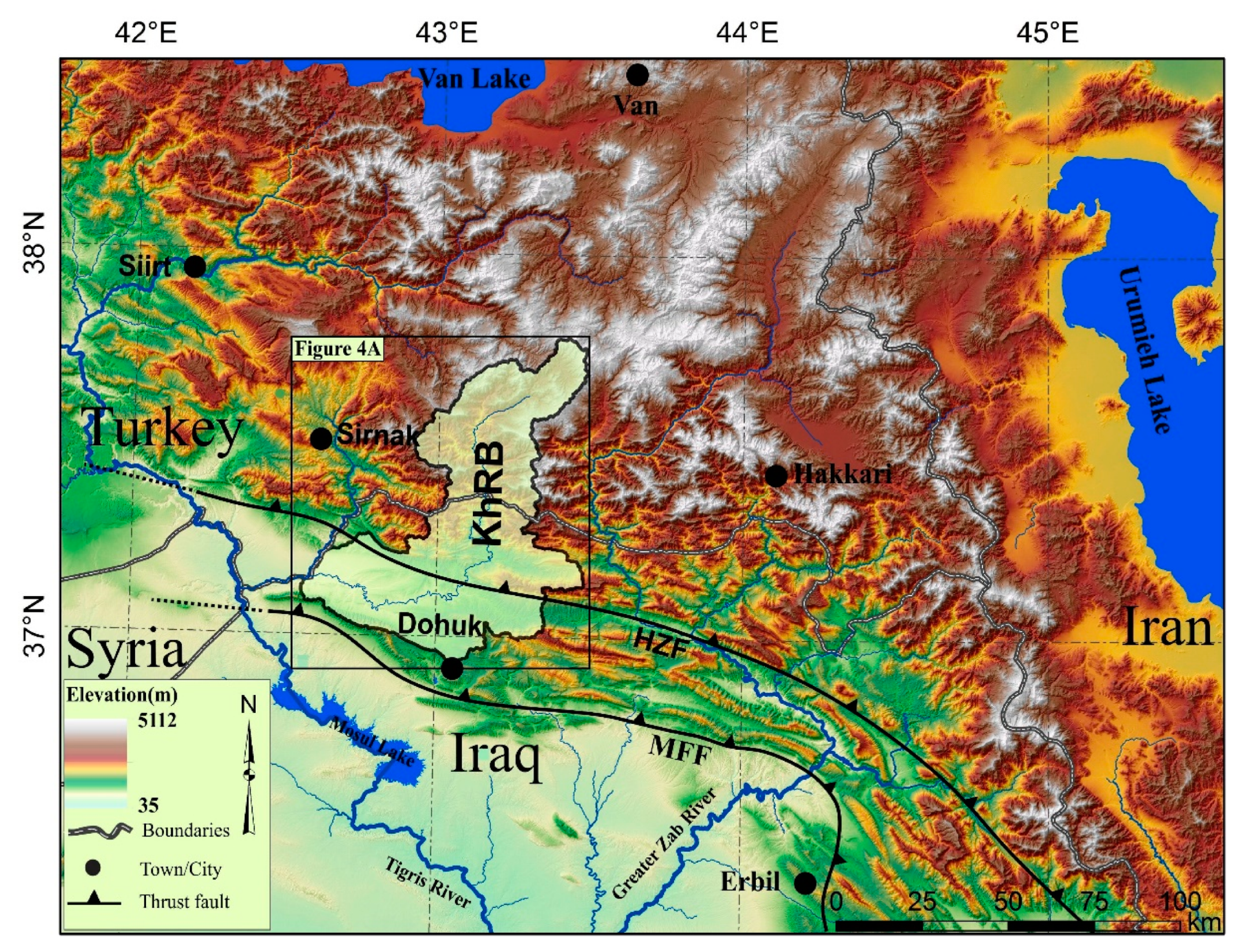
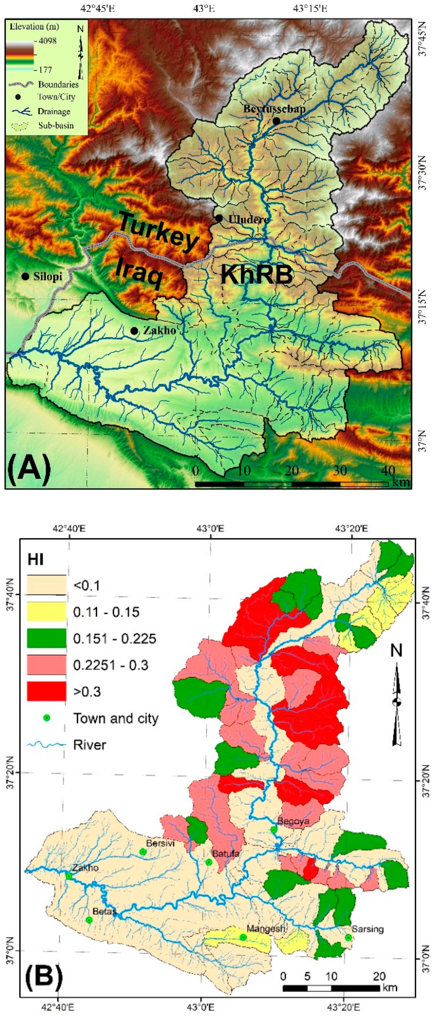
2.1. Study Area

The study area is located at the distal northwestern part of the ZFTB between 36°55′28″–37°47′01″ N latitudes and 42°34′44″–43°29′5″ E longitudes, along the border between Iraq and Turkey. It encompasses an area of ~3500 km2 and represents the Khabur River Basin (KhRB). The area is characterized by rugged topography and high relief to the north, due to the presence of the High Zagros Fault (HZF), and subdued topography and low relief in the southern part, near Dohuk city (Figure 1). The area is characterized by its remoteness and difficulty of access, frequent landslides and lacks useful in situ hydrological and pedological information. The area encompasses the Khabur River that is the source of life-sustaining water to the region. The Zakho meteorological station data indicate significant seasonal fluctuation in the region, characterized by long, dry summers and short, rainy winter conditions. Most of the precipitation (586 mm) occurs between October and May, with a maximum monthly average of 134.3 mm occurring in January. The monthly average temperature and evaporation occurs in July, 33.96 °C, and 354.7 mm, respectively, and the minimum temperature of 4.17 °C was recorded in January (Figure 2).
A number of dams have been planned in the KhRB and, like the existing Mosul dam with a high rate of reservoir siltation at 78,000 t.ha−1.y−1 [59]. Excessive soil erosion in the region would create a major problem for the proposed dams, as pointed out by [48]. The rate of soil loss determined by this study will, therefore, enable the decision makers to incorporate suitable soil conservation measures to mitigate reservoir siltation problem, and also to optimize agricultural productivity.

2.2. Data and Software

We used four scenes of the mosaicked Digital Elevation Model (DEM), with 30 m spatial resolution (1 arc-second), gathered by Shuttle Radar Topography Mission (SRTM) [60]. DEM was used to extract the drainage network and calculate the slope and runoff flow accumulations. Due to the lack of in situ meteorological data, we employed Tropical Rainfall Measuring Mission (TRMM) data [61] to produce the rainfall map. The TRMM (3B43-V7) is a raster structure with 0.25° × 0.25° spatial resolution that collects monthly precipitation data [62]. The Harmonized World Soil Database (HWSD) [63] was used to determine soil erodibility, or the K factor. It has a cell size of 30 arc-second (~1 km). We combined seasonal impacts on vegetation using four Landsat Operational Land Imager (OLI) scenes. These scenes in Level 1T format, acquired in 2019, were used in this study. Details are listed in Table 1. The spectral images are of good quality, geo-referenced, and orthorectified with a 30 m spatial resolution, and are available without any charge, from the Earth Resources Observation and Science (EROS) center in Sioux Falls, South Dakota, U.S.A. Only scenes with excellent quality and less than 12.5 % cloud cover were chosen for this study. The region of interest is positioned in zone 38 north and the path and row of the image are 170 and 34 respectively. All input data were reprojected to the Universal Transverse Mercator (UTM) projection/WGS 1984 datum, within zone 38N using the nearest neighbor resampling method to fit with the OLI scenes.
Combining the powerful capabilities of remote sensing and GIS, and using multiple datasets from different sources [64], we applied the RUSLE model to estimate soil loss in the study area. We used the MATLAB based TecDEM 2.2 [65,66] software to extract the drainage network. Specific functions within the ArcGIS 10.3 [67], such as slope, runoff flow accumulation, interpolation, raster conversion, and raster calculator, were utilized for base map preparation. In addition, we used Environment for Visualizing Images (ENVI) software for Landsat imageries preparation and processing that included implementing Boolean operation, surface reflectance conversion, and Normalized Differential Vegetation Index (NDVI) determination. R-studio script was used for statistical analysis.

2.3. Hypsometric Integral (HI)

The HI is a useful metric to identify different stages of landscape development in its geomorphological erosion cycle [12,68,69]. We used HI to determine the stage of landscape development (erosional stages) to quantify the relationship between HI and amount of soil loss. The mature (highly eroded) areas have low HI values, while the youthful (slightly eroded) areas show high HI values [12,14,69,70,71,72]. According to [73], the HI of a given area can be estimated using Equation (1):
H I =   H m e a n H m i n H m a x H m i n
where H m a x , H m i n , and   H m e a n are the maximum, minimum, and mean elevations, respectively.
An HI value close to 1 means that the terrain removal is in the lowest stage (uplift > erosion) and the land surface is in its youthful stage, while low HI values (close to 0) refers to high amount of terrain removal (erosion > uplift) and the land surface is in its mature stage. This dimensionless parameter is very useful for comparing the erosional stage of different basins regardless of their size (areas).

2.4. RUSLE Model Description

The RUSLE model, proposed by [41], can been used to estimate annual soil loss as shown in Equation (2).
A E = R   .   K   .   L S   .   C   .   P
where,
  • AE is the actual erosion (yearly rate of the soil loss (t.ha−1.y−1));
  • R rainfall and runoff erosivity factor (MJ.mm.ha−1.h−1.y−1);
  • K, soil erodibility factor (t.ha.h.ha−1.MJ−1.mm−1);
  • LS, the slope length and slope steepness factor;
  • C, the cover management factor;
  • P, the support practice factor;
  • LS, C, and P factors are dimensionless.
The following sections explain the method of calculating RUSLE factors.

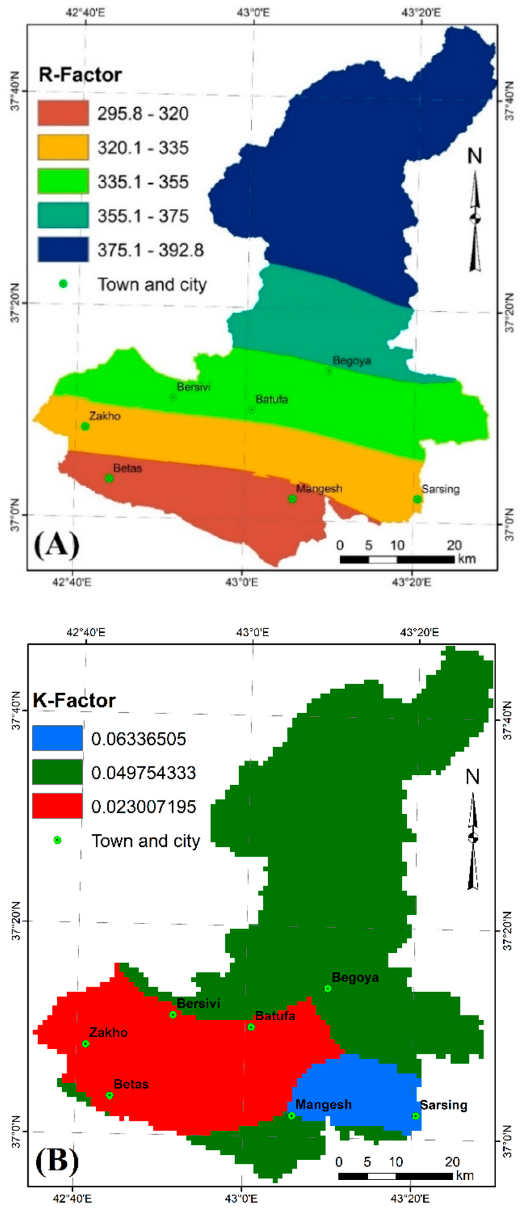
2.4.1. Rainfall and Runoff Erosivity (R factor)

The R factor expresses the effect of precipitation on soil erosion [74,75], as soil particle detachment is directly related to precipitation [76]. Estimation of R factor requires the availability of accurate and continuous precipitation data [22,31].
Since the study area lacks reliable meteorological data, we used the monthly TRMM (3B43-V7) to calculate the yearly average precipitation (mm), due to its suitable temporal and spatial resolution [30], and because of its extensive application for assessing the R factor, as compared to other satellite data. The TRMM data covers 15 years between September 2002 and August 2017. The TRMM pixels have been changed in vectors (points) format, and these points were interpolated employing an Inverse Distance Weighting (IDW) method, to produce a raster format with a spatial resolution of 30 m.
Numerous approaches have been used to calculate the R factor by employing long-term precipitation data. [77] found that Equation (3) can be used to calculate the R factor, which is directly related to the average annual rainfall.
R = 81.5 + 0.38   P A
where R is the rainfall erosivity factor in MJ.mm.ha−1.h−1.y−1 and P A is the average annual precipitation in mm.
Precipitation in the KhRB amounts to 562.85 mm∙yr−1 in the south, increasing to 785 mm∙yr−1 to the north. The suitability of applying TRMM data in the study area was evaluated by comparing it with the observed precipitation dataset of Zakho meteorological station. Sixty-two monthly precipitation measurements, covering the period from September 2002 to December 2007 were compared with the TRMM data (Figure 3). In this figure, a strong direct relationship was found, the coefficient of determination (R2) being 0.853, at a significant p-value of <0.05. The slope and intercept were 0.9124 and 9.5485, respectively.

2.4.2. Soil Erodibility (K) Factor

The K–factor representing soil vulnerability to erosion, is affected by rainfall and runoff, [30,78]. Soil susceptibility to erosion is affected by its physical and chemical characteristics, such as its texture, mineralogy, and structure. Five soil parameters (i.e., texture, organic matter content (OM), coarse fragments, structure, and permeability) are the main properties that influence the K–factor. With the soil OM being inversely proportional to soil erodibility, such that any increase in soil OM decreases its vulnerability to detachment [36]. For this study, dataset of the HWSD was used to obtain information about soil texture and soil organic carbon (OC). We used Table 2 and Table 3 to estimate the soil structure class and the soil permeability class, respectively [22,79]. We estimated the K–factor of the soil types in the study area using Equations (4) and (5) [22,79].
K = [ 2.1   × 10 4   M 1.14   ( 12 O M ) + 3.25 ( s 2 ) + 2.5 ( p 3 ) 100 ] 0.1317
M = ( m s i l t + m v f s ) ( 100 m c )
mc [%] is clay fraction (<0.002 mm);
msilt [%] silt fraction (0.002–0.05 mm);
mvfs [%] very fine sand fraction (0.05–0.1 mm);
OM [%] the organic matter;
s is the soil structure class (s = 1: very fine granular, s = 2: fine granular, s = 3, medium or coarse granular, s = 4: blocky, platy or massive; Table 2);
p is the permeability class (p = 1: very rapid, …, p = 6: very slow; Table 3).
Estimating soil OM from the organic carbon (OC) is a simple procedure but requires the use of a conversion factor [80]. However, there is no agreement on the conversion factor [81] to use for converting soil OC to OM [82]. According to [80,82], a more reliable value of OM can be obtained by using the conversion factor of 1.724, which is based on the assumption that soil OM contains 58% carbon, as shown in Equation (6).
O M = 1.724 O C

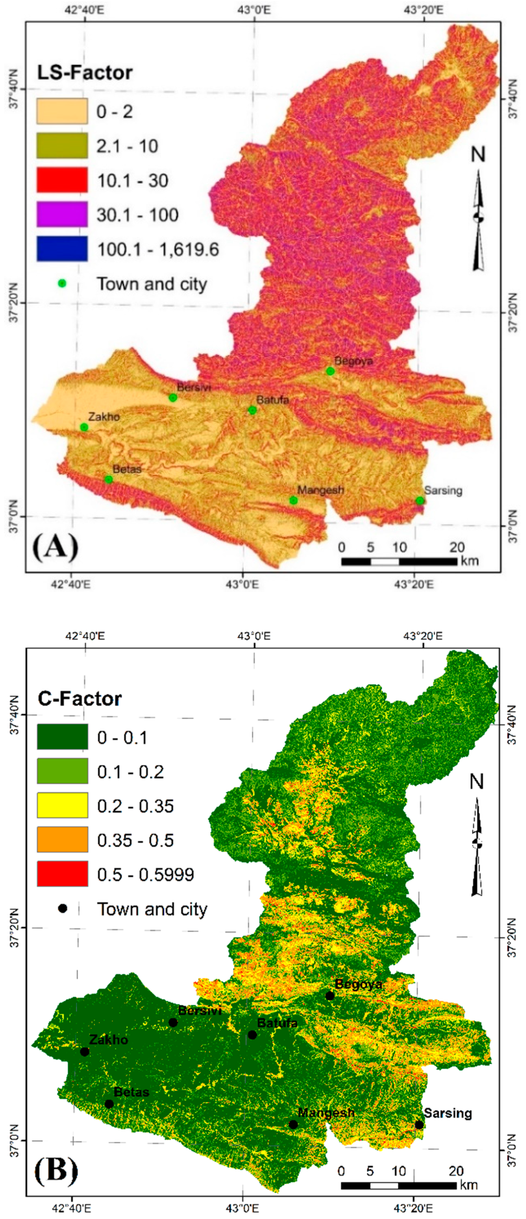
2.4.3. Slope Length and Slope-Steepness Factor (LS factor)

The LS factor which is a function of slope length (L) and slope steepness (S), reflects local topography’s influence on soil erosion. Numerous approaches have been proposed to evaluate the LS factor (e.g., [22,23,36,83,84,85,86]. We have estimated the L factor using Equations (7)–(9) proposed by Moore and Burch (1986).
The L factor can be computed by using a slope (in percent) and runoff flow accumulation. We divided the slope map into four classes, which are <1%, 1–3%, 3–5%, and ≥5%.
L = ( λ 22.12848 ) m
λ = FA Ps
λ = FA Ps
where, λ is the horizontal projection of slope length (m), m is a constant, based on the value of slope; FA is runoff flow accumulation, Ps is the cell size of DEM, and θ is the slope angle in percent.
We estimated the S factor by dividing the slope (in percent) into three classes: <9%, 9–18%, and ≥18% (Equation (10). Equation (11) was applied to evaluate the LS factor.
S = { 10.8 . s i n θ + 0.03                                                       θ < 9 % 16.8 . s i n θ 0.05                         9 %   θ < 18 % 21.9 . s i n θ 0.96                                                     θ 18 %
L S = L S
where S is the slope steepness factor, θ is the slope angle in percent, and L S represents the slope length and slope steepness factors [87].

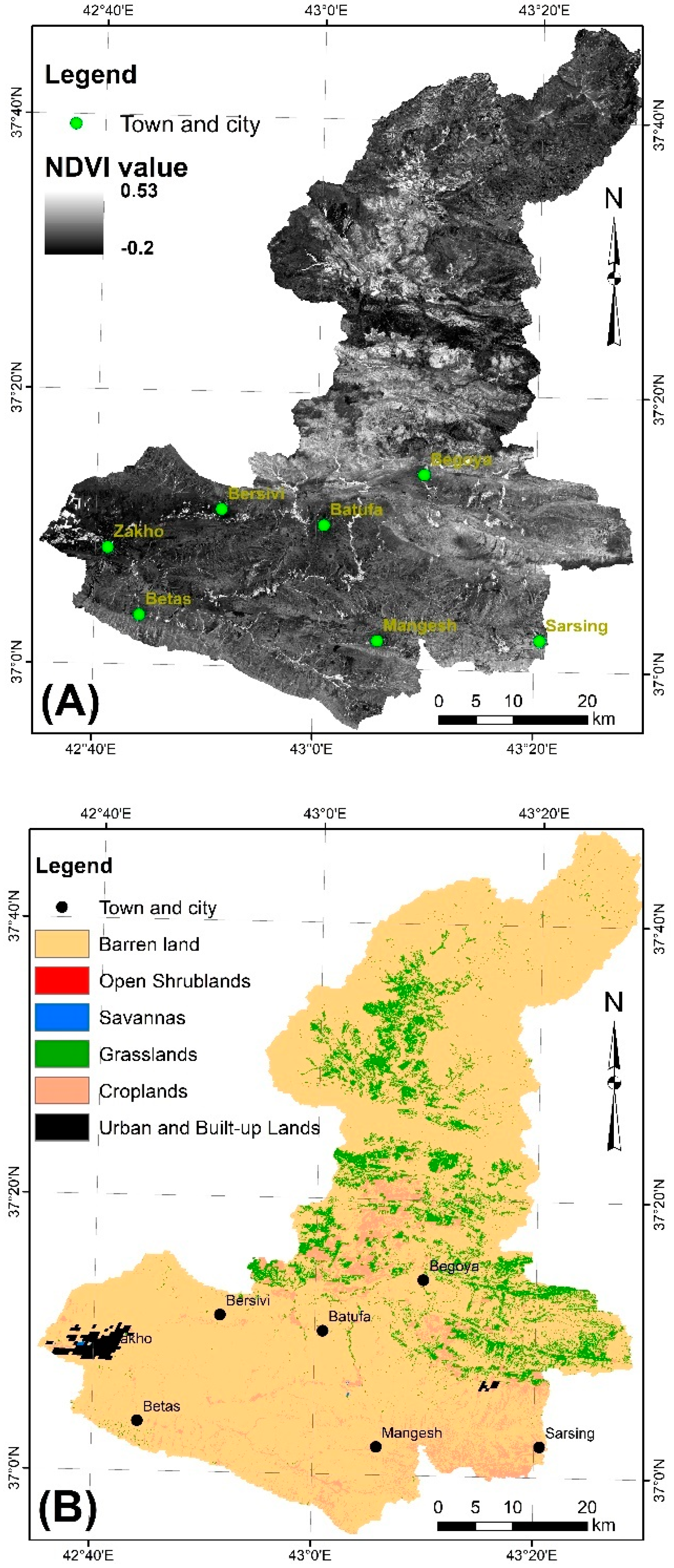
2.4.4. Cover and Management Factor (C factor)

As a dimensionless and influential factor used in the RUSLE model, the C factor refers to the amount of soil erosion related to the degree of vegetation/ground cover. Evaluation of vegetation cover is considered the most significant aspect of estimating the C factor [88].
We first performed the radiometric corrections to compute top of atmosphere reflectance ( ρ ) by using (Equation (12)).
ρ =   π L λ D 2 ( E s u n , λ c o s   ( θ ) ) 1
where ρ is reflectance (at sensor), Lλ represents at-sensor radiance, D is sun–earth distance in astronomical units, θ is the solar zenith angle, and Esun,λ is the solar spectral irradiance. Next step involved atmospheric corrections that were performed using the Fast Line-of-Sight Atmospheric Analysis of Spectral Hypercubes (FLAASH) model. The FLAASH [89] model is based on a MODTRAN4 model to decrease the molecular and particulate scattering, absorption, and adjacency effects to retrieve at-surface reflectance values ( ρ ) [90,91,92]. The surface reflectance ( ρ ) of the OLI imageries is used to compute NDVI following Equation (13) [93], which, in turn, was used to compute the C factor using Equation (14) [94,95,96].
N D V I = ρ N I R ρ R ρ N I R + ρ R
where ρ N I R and ρ R are the reflectance of band 5 (851 nm–879 nm) and band 4 (636 nm–673 nm) of the Landsat-8 OLI surface reflectance.
C = E x p [ α N D V I ( β N D V I ) ]
where α , β are constants, which were deduced from [94,95] to be 2 and 1, respectively. These constants determine the shape of the NDVI–C curve. We omitted the bare rock in the soil loss assessment, affirmed by relatively low values of NDVI [32].

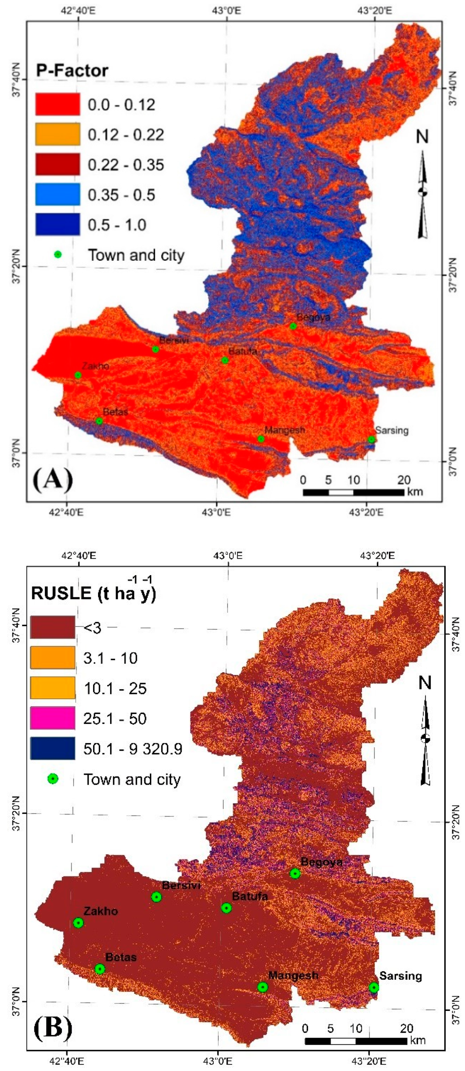
2.4.5. Support Practice Factor Related to Slope Direction (P)

The P factor describes soil loss ratio by a specific soil conservation or support practice to the corresponding loss up– and down–slope [23,97]. Lack of in situ data for conservation practices within the Zagros region prompted us to apply Equation (15) for estimating the P factor. We modified Equation (15) as suggested by Wener [33,37,98] and used the modified equation (Equation (16)) to calculate P.
P = 0.2 + 0.008 θ
P = 0.2 + 0.03 θ
where, P is the support practice factor, θ is the slope angle in percent. By applying Equation (16), the P factor of flat pixels ( θ = 0) was found to be 0.2 (i.e., P = 0.2 + 0.008 * 0), and for the highest slope angle pixels ( θ = 100) it was 1 (i.e., P = 0.2 + 0.008 * 100).

2.5. Sediment Yield (SY)

We estimated the SY in the KhRB following [99]. First, we measured the areas of the sub-basins within the KhRB. Then, we calculated the SDR (Equation (17)). Finally, we estimated the SY amount for each sub-basin following Equation (18) [99]. Results of SY were used to estimate the amount of sediment transported by streams and rivers to the downstream area to determine the check dam locations.
S D R = 1.817 × A b 0.132
S Y = A E × S D R
SDR is sediment delivery ratio;
Ab is area of a basin (km2);
AE is the actual erosion (yearly rate of soil loss (t.ha−1.y−1));
SY is the sediment yield (t.ha−1.y−1).

2.6. Work Procedure

We applied the RUSLE model to estimate soil loss for the KhRB. The KhRB was subdivided into a number of sub-basins (Figure 4A). We estimated the mean of the AE, the PE, and the mean of the HI, for each sub-basin (Figure 4B). Afterwards, we tested the relationship between AE and PE for them.
We classified various parameters in the RUSLE model into five classes, using the natural breaks technique, except the K factor that was classified into three classes based on the three soil types present in the KhRB. These classes are: very high, high, moderate, low, and very low. The natural break classification is best applied to familiar data ranges. It reduces the variance within classes and maximizes the variance between classes [72,100]. This characteristic makes the natural breaks useful when RUSLE and its factors histogram show distinct breaks.

3. Results

3.1. The Hypsometric Integral (HI)

Figure 4B displays the HI for the study area. The HI values range from 0.36 to 0.05; low values (<0.30) were obtained for the central and lower parts of the KhRB, indicating plain terrain with occasional slope. The HI values above 0.30 fall in the part of basin located inside Turkey. The topography of these areas possesses high relief, which might be controlled by the active thrust fault, HZF (Figure 1).

3.2. The R Factor

The value of R factor in the study area varied from ~296 to ~393 MJ.mm.ha−1.h−1.y−1, with an average of ~354 MJ.mm.ha−1.h−1.y−1. The R factor map of KhRB, presented in (Figure 5A), has been sliced into five groups, to show relatively lower R factor values in the south of the KhRB compared to the mountainous terrain in the north.

3.3. K Factor

The K factor data presented in Figure 5B show that the minimum and maximum soil erodibility is ~0.023 t·ha·h·ha−1·MJ−1.mm−1 in the southwestern part of the KhRB and ~0.063 t·ha·h·ha−1·MJ−1.mm−1 in the southeastern parts of the KhRB respectively. Major part of the basin has an intermediate to high K value (~0.0498) occurring in the central and northern part of the basin. Three types of soil occur in the KhRB: lithosols, calcic xerosols, and chromic vertisols. The textural description and the K–factor for each soil type is shown in Table 4 and Figure 5B. Variations in the K–factor values are possibly due to variations in the soil types’ physical characteristics.

3.4. The LS Factor

The highest slope angle in the KhRB is 77°, the average being 17.5°. Nearly all high slope areas are located in the central and northern parts of the KhRB. Due to the difference in runoff flow accumulation, and slope distribution, the LS factor values range from 0 to 1619.6 with the average and standard deviation 12.05 and 12.74, respectively (Figure 6A). The KhRB, generally, is characterized by moderate LS factor values: It is <10 in the lower part of the KhRB, but the middle and upper parts of the basin show relatively higher LS factor values, which indicate the possibility of greater soil erosion and consequently accelerated land degradation.

3.5. The C Factor

The C factor ranges from 0 to 0.5999 (Figure 6B). Less than 16% of the KhRB is covered with vegetation, and most of the barren land occurs in the upstream and downstream parts of the basin (Figure 7A) where C factor values are low (dark green and green colors). Presence of vegetation increases soil particles’ adhesion and binding, making it less prone to erosion. The moderate, high, and very high (>0.2) values of the C factor (green, orange, and red colors) are mainly restricted to the midstream part of the KhRB. Four types of vegetative areas exist in the KhRB (Figure 7B). Open shrublands (dominated by woody perennials (1–2 m height), 10–60% cover), savannas (tree cover 10–30% (canopy > 2 m)), grasslands (dominated by herbaceous annuals (<2 m)), and croplands (at least 60% of area is cultivated cropland) [101].

3.6. The P Factor

Values of the P factor within the KhRB range between 0 and 1 (Figure 8A). Low values correspond to pixels with good conservation practice, while the high values denote areas of poor conservation practice [31]. P factor value depends on slope length and steepness, and farming method [102]. Therefore, an increase in the value of P factor is consistent with the rise in the LS factor value (Figure 6A and Figure 8A). High and very high (0.35–1) values of P factor are mainly distributed in the middle part of the KhRB, while the low and very low values (0–0.22) are mainly distributed downstream of the KhRB (Figure 8A).

3.7. Estimation of Soil Loss

We integrated the RUSLE model’s parameters within the GIS environment to evaluate the average annual soil loss in the KhRB and estimate it to be 11.16 t.ha−1.y−1 (Figure 8B). The minimum and maximum yearly soil losses are 0 t.ha−1.y−1 and 3617.6 t.ha−1.y−1, respectively. Total annual soil loss for the whole study area is estimated at 31,237,283.358 t.y−1. The low and very low range (<10 t.ha−1.y−1) of the yearly soil loss values mainly occur in the northeastern and downstream reaches of the KhRB, while the moderate, high and very high range (>10 t.ha−1.y−1) occurs in the midstream and upstream parts of the KhRB (Figure 8B). Very high soil losses (>50 t.ha−1.y−1) occur only in 6.19% of the KhRB.

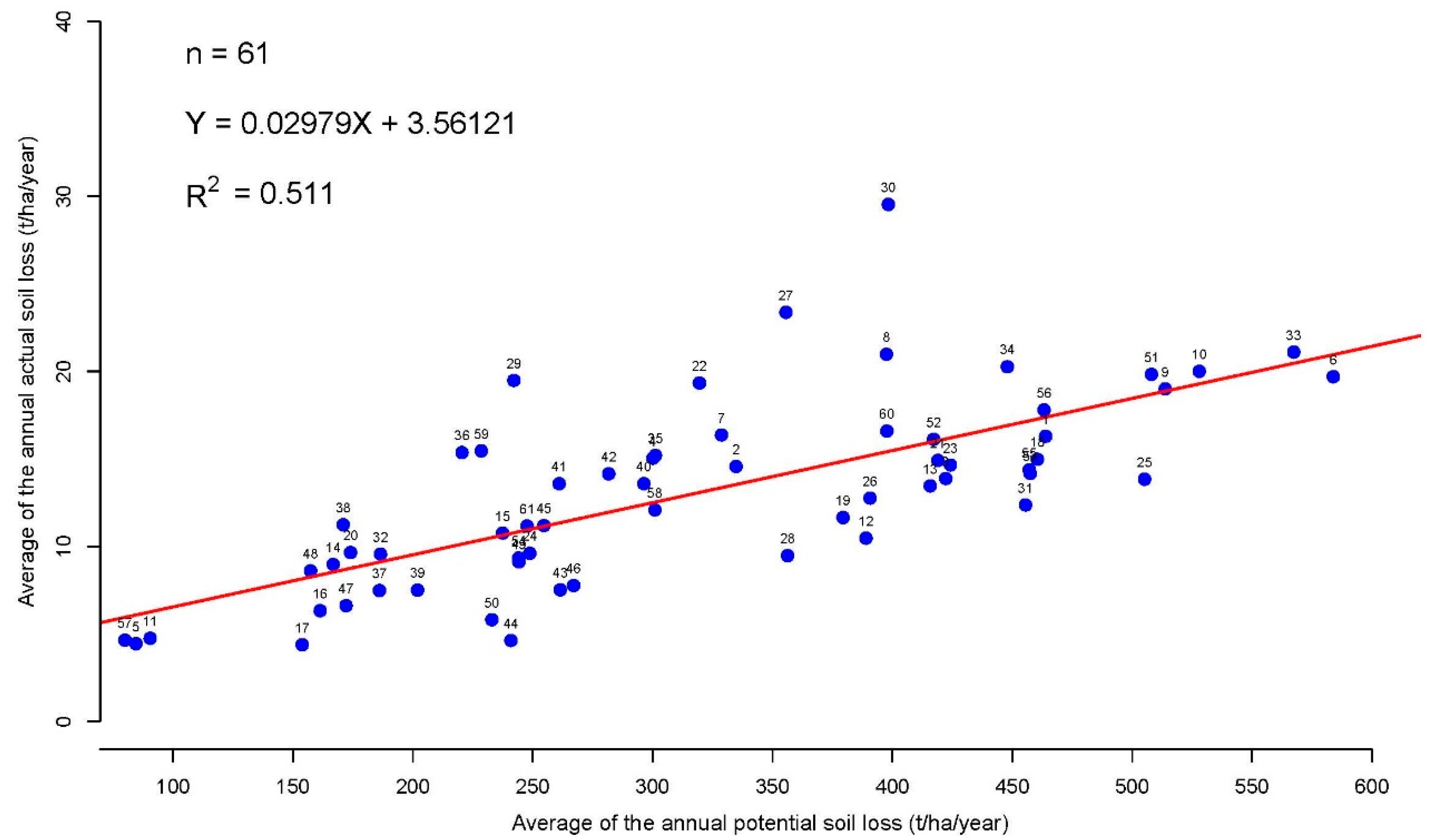
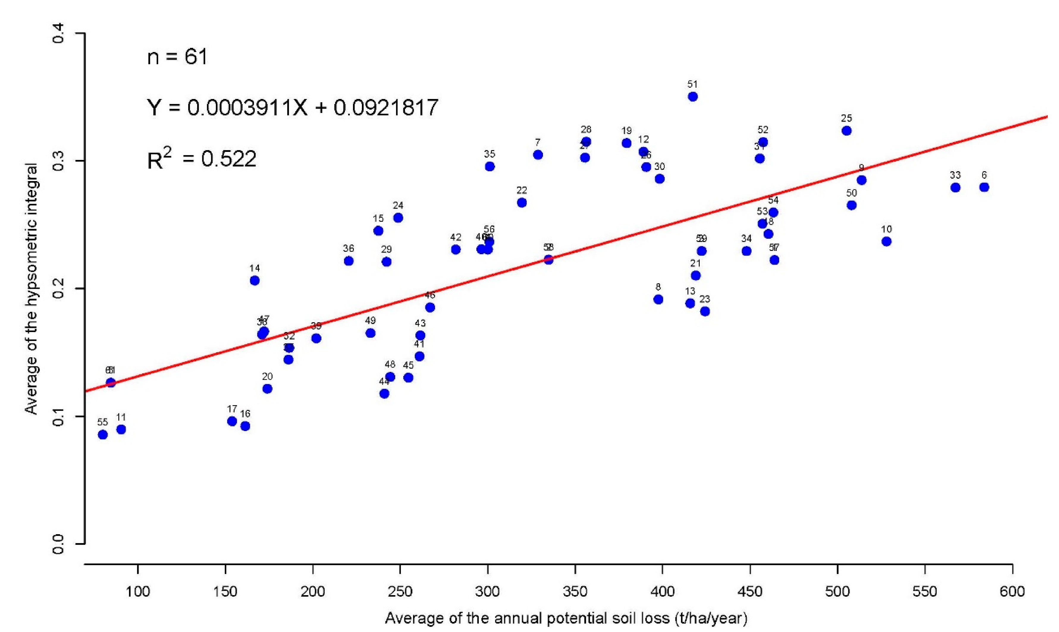
3.8. Relationship of PE to RUSLE and the HI

Our study revealed a strong direct correlation between: (a) PE and soil loss, and (b) PE and HI. It is well recognized that heavy rain, and steeper slopes contribute to a large volume of runoff with high erosive energy and greater amount of soil loss. Sixty-one sub-basins included in the KhRB, comprise areas ranging between 3.5 and 974.6 km2 (average: 57.5 km2). Analyses of annual soil loss within the KhRB at the sub-basin scale reveal a moderate linear relationship between the mean of the PE and mean of soil loss. This direct relationship is clearly displayed in Figure 9, where the statistical correlation, the p-value, the t-test, the slope, and the intercept of the data were >0.511, 9.572 × 10⁻¹¹, 7.8565, 0.02979, and 3.56121, respectively. Using the same procedure, we found a moderate linear relationship between the mean of HI and mean of soil loss (Figure 10), where the statistical correlation, the p-value, the t-test, the slope, and the intercept of the data were 0.522, 3.315 × 10⁻¹⁰, 7.6743, 0.0003911, and 0.0921817, respectively.

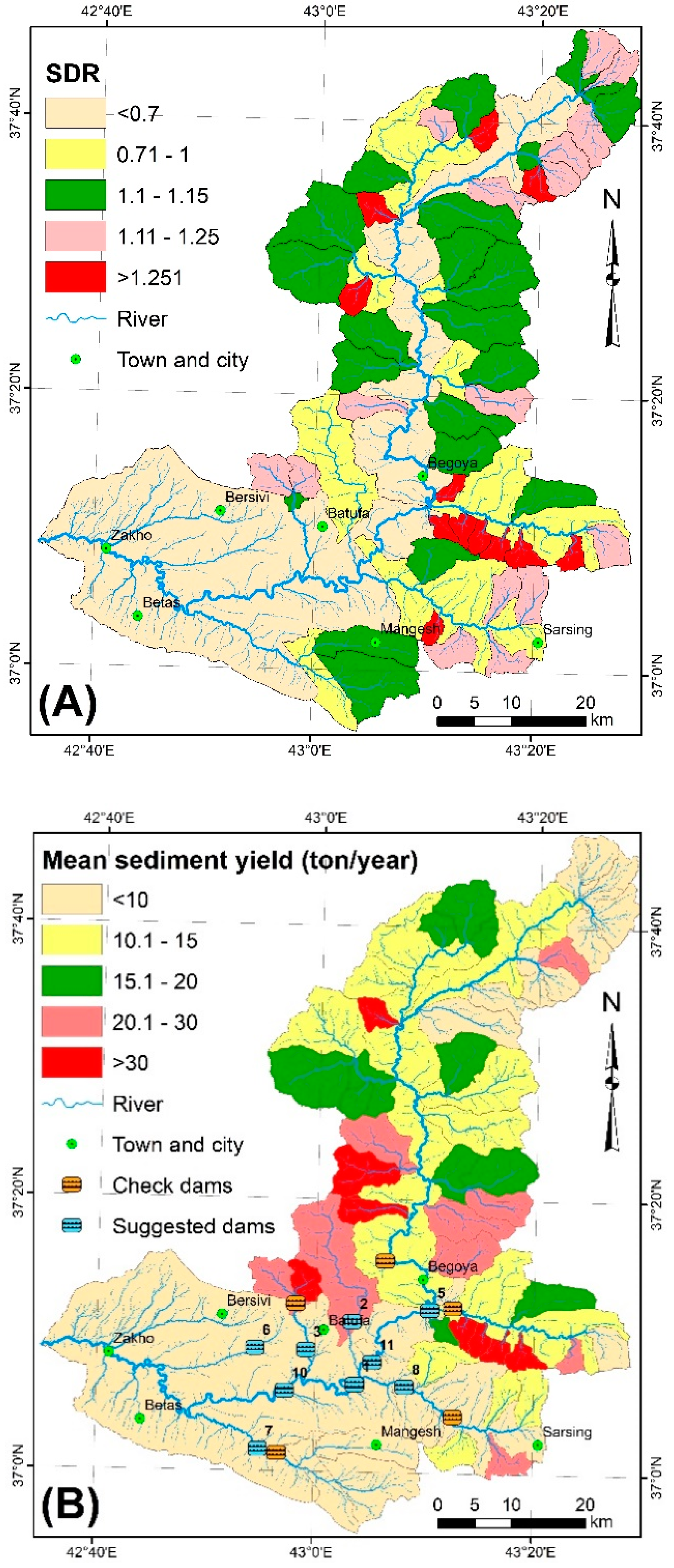
3.9. Estimation the Sediment Yield

In addition to SDR (Figure 11A), we also calculated the average annual quantity of SY for the 61 sub-basins included in the KhRB. The SDR values range between 0.619 and 1.373, respectively. Estimate of the yearly average of SY in the KhRB is 57.79 t.y−1. The minimum and maximum yearly SY are 6.9 t.y−1 and 165.12 t.y−1, respectively. Total annual SY for the whole study area is estimated at 21,817.68 t.y−1. The low and very low range (<10 t.ha−1.y−1) of annual SY values mainly occur in the northeastern and downstream reaches of the KhRB, while the moderate, high and very high range (>10 t.ha−1.y−1) occur in the midstream part of the KhRB (Figure 11B).

4. Discussion

It is well established that soil loss is controlled by the five factors of the RUSLE model (i.e., R, K, LS, C, and P). Change in one of these factors leads to a change in the quantity of soil loss. As can be seen in Equation (3), the R factor is directly related to the amount of precipitation [77]. Moreover, in the KhRB, precipitation is affected by elevation (Figure 1). The soil loss is a function of K factor, rainfall, and runoff [30,78]. The higher the K factor, the greater is the amount of soil loss and vice versa [103]. The same is true for the LS factor, where the amount of soil loss increases with increasing LS factor and vice versa [85,87]. Our results show moderate to high soil loss in areas with high R factor values (Figure 5A), which is consistent with relatively steeper slope zones (Figure 6A and Figure 8B). Soil loss is a function of the products of all five factors in RUSLE, of which R, K, LS are natural factors and cannot be changed, P and C are factors that can be altered by human intervention. This is precisely what is done to minimize soil loss in agricultural land [104,105]. Therefore, by taking measures to reduce values of P and C factors by contour ploughing, no-till seeding, and terracing, etc. the overall soil loss can be reduced.
The C factor is relatively lower in the southern part of the KhRB (Figure 6B) because of sparse vegetation, somewhat gentler slopes, and lower rainfall amounts–all of which contribute to lower rate of soil loss (Figure 8B). On the other hand, the central and the northwestern parts of the KhRB, with lower values of the C factor, due to presence of vegetation, exhibit a relatively higher amount of soil loss due to relatively steeper slope and higher amounts of rainfall. Dynamics of the erosional process are greatly affected by the LS factor that controls runoff flow. Our results agree with the findings reported by [106] in which the altitude variance and topographic relief control the LS factor (Figure 6A); and higher value of P factor (Figure 8A) directly correlates with a higher rate of soil loss (Figure 8B). Interestingly, both of which are related to the steeper slopes (Figure 6A).
This study also concurs with [8], which stated that the main factor controlling soil loss “in the NW part of the ZFTB” is the LS factor (Figure 6A). The next important factor that affects soil loss is the R factor (Figure 5A). There is a narrow range in the values of the K factor (~0.023–0.063 t·ha·h·ha−1·MJ−1.mm−1), C factor (0.2–0.87), P factor (0–1), and R factor in the sub-basins. The LS factor for ~99% of the pixels in the sub-basins gave values of <166, except some that show an extremely high value of about 1500.
From the above discussion of the various RUSLE parameters, it can be stated that slope is the main proxy that controls soil loss in the region, where precipitation is strongly affected by the slope. Regional tectonism, evidenced by the presence of HZF in the study area (Figure 1), is believed to have contributed to development of steeper slopes.
Although the RUSLE model is widely used to quantify soil loss and may be more accurate than other methods [107], it has not been applied at pixel scale to estimate PE in the study area. Our study revealed direct relationship between potential soil loss and actual soil loss at the sub-basin scale, but a with moderate-strong value of 0.51 for the coefficient of determination, R2 (Figure 9). This may be due to the difference in precipitation, soil types, and vegetation density in the various sub-basins.
Overall, this study shows that soil loss in the study area increases with an increase in slope angle, rainfall, and lack of vegetation, and is more pronounced in regions of steeper slopes. This study agrees with [108], which reported that different slopes initiate different rates of soil loss, and progressively higher soil loss occurs on steeper slopes. Our study indicates that the direct relationship between PE and HI can be formed in quantitative relationships (Figure 10). This relation confirms the finding of [14,71] that the sub-basins in youthful stage are more active than mature stage. This allows the determination of active and inactive erosional regions, which will be helpful to select the best sites for check dams.
Further studies should be carried out to ensure safety of existing dams in Iraq. Regarding potential siltation problems in the proposed dams in Iraq, research should be undertaken to determine annual volume of soil that will enter the reservoirs to ensure safety and longevity of the planned structures.

Estimation of the Dam Siltation in the KhRB

Estimation of soil loss at sub-basin scale provided reliable data to find suitable sites for locating main dams and the check dams. We applied RUSLE with GIS and RS at the sub-basin scale for the first time in the KhRB to estimate soil loss. Since the planned dams are located in the sub-basins (Figure 11B, Table 5), they would experience excessive reservoir siltation due to high rate of soil loss. To minimize this problem, we have recommended check dams to trap the sediments upstream of the main dams.
One of the common and simple ways to mitigate excessive siltation is construction of small check dams. [48] had recommended suitable locations for dams in the KhRB (Figure 11B and Table 5) based on lithology, tectonic zones, distance to active fault, distance to the lineaments, soil type, land cover, elevation, slope gradient, precipitation, stream width, curve number, distance to road, distance to towns and cities, and distance to villages [109,110,111]. These dam sites might be influenced by soil loss from the upstream areas leading to excessive reservoir siltation. Drawing upon our present research, we propose construction of five check dams to trap sediments transported from the upstream area of the KhRB (Figure 11). These dams will prevent ~1757 t.y−1 of sediment, eroded from the upper reaches of the KhRB, from entering the main dams. The suggested check dams will prolong the lives of proposed dams (Figure 11B), and also increase the useful life of the Mosul dam to the southwest of the KhRB.

5. Conclusions

The classical RUSLE model has been integrated with remote sensing and GIS to estimate soil loss and sediment yield in the KhRB. Results show the spatial distribution and rate of average annual soil loss and sediment yield within selected basins that ranges from 0 t.ha−1.y−1 to 3617.6 t.ha−1.y−1, and from 6.9 t.y−1 to 165.12 t.y−1, respectively. The northwestern part of KhRB experiences low rate of soil loss (A) and SY. These rates are mainly influenced by topography, characterized by steep slopes, and high rainfall. Our study also demonstrates that LS and R are the most dominant factors controlling soil loss in the selected area. Analysis of the potential and actual soil erosion for KhRB shows a direct relationship. We conclude that RUSLE can serve as an effective model for estimating sediment yield, and for mitigation its adverse effects on multi-purpose river valley development projects for water supply, agriculture, etc. We recommend locating check dams in the upstream reaches of KhRB to minimize reservoir siltation and ensure safety of the main dams. Our study showed a correlation between potential soil erosion and HI. We found that HI values at the sub-basin scale can be used to identify active and inactive erosional regions. Thus, HI could serve as a useful geomorphic index for locating check dams in basins with high rate of soil loss. Further studies should be performed to find out if the HI can be used for estimating actual soil loss at specific locations.

Author Contributions

Arsalan Ahmed Othman outlined the research, prepared and processed the data, accomplished the study, and wrote the manuscript. Ahmed K. Obaid processed the data and supported the writing, analysis, and discussion. Diary Ali Mohammed Amin Al-Manmi, Ahmed F. Al-Maamar, Ahmed T. Shihab, and Younus I. Al-Saady supported the analysis and RUSLE model. Veraldo Liesenberg and Syed E. Hasan supported the writing and discussion. All authors have checked and revised the manuscript. All authors have read and agreed to the published version of the manuscript.

Funding

This research received no external funding. Veraldo Liesenberg is supported by FAPESC (2017TR1762) and CNPq (313887/2018-7).

Institutional Review Board Statement

Not applicable.

Informed Consent Statement

Not applicable.

Data Availability Statement

Data available on request due to privacy restrictions.

Acknowledgments

We thank USGS for providing Landsat and DEM data. We are grateful to the General Survey Authority and Ministry of Planning, Iraq for providing other useful data used in our study. We would like to thank the Food and Agriculture Organization (FAO) of the United Nations, Chinese Academy of Sciences (CAS), International Institute for Applied Systems Analysis (IIASA), International Soil Reference and Information Centre (ISRIC), and Joint Research Centre of the European Commission (JRC) for supplying Harmonized world soil database (HWSD). We are grateful to the U.S. National Aeronautics and Space Administration (NASA) and the Japan Aerospace Exploration Agency (JAXA) for providing Tropical Rainfall Measuring Mission (TRMM) data.

Conflicts of Interest

The authors declare no conflict of interest.

References

  1. García-Ruiz, J.M.; Beguería, S.; Nadal-Romero, E.; González-Hidalgo, J.C.; Lana-Renault, N.; Sanjuán, Y. A meta-analysis of soil erosion rates across the world. Geomorphology 2015, 239, 160–173. [Google Scholar] [CrossRef] [Green Version]
  2. Pimentel, D.; Terhune, E.C.; Dyson-Hudson, R.; Rochereau, S.; Samis, R.; Smith, E.A.; Denman, D.; Reifschneider, D.; Shepard, M. Land degradation: Effects on food and energy resources. Science 1976, 194, 149–155. [Google Scholar] [CrossRef] [PubMed]
  3. Othman, A.A. Improving Remote Sensing Based Landslide Investigations and Lithological Mapping Using Morphological Features: A Case Study in NE-Iraq and W-Iran; Technische Universität Bergakademie: Freiberg, Germany, 2015. [Google Scholar]
  4. Kuzucuoğlu, C.; Çiner, A.; Kazancı, N. (Eds.) The Geomorphological Regions of Turkey BT. In Landscapes and Landforms of Turkey; Springer International Publishing: Cham, Switzerland, 2019; pp. 41–178. ISBN 978-3-030-03515-0. [Google Scholar]
  5. Carretier, S.; Regard, V.; Vassallo, R.; Aguilar, G.; Martinod, J.; Riquelme, R.; Pepin, E.; Charrier, R.; Hérail, G.; Farías, M.; et al. Slope and climate variability control of erosion in the Andes of central Chile. Geology 2013, 41, 195–198. [Google Scholar] [CrossRef]
  6. Al-Saady, Y.; Al-Suhail, Q.; Al-Tawash, B.; Othman, A. Drainage network extraction and morphometric analysis using remote sensing and GIS mapping techniques (Lesser Zab River Basin, Iraq and Iran). Environ. Earth Sci. 2016, 75. [Google Scholar] [CrossRef]
  7. Othman, A.A.; Al-Maamar, A.F.; Al-Manmi, D.A.M.; Liesenberg, V.; Hasan, S.; Al-Saady, Y.I.; Shihab, A.T.; Khwedim, K. Application of DInSAR-PSI Technology for Deformation Monitoring of the Mosul Dam, Iraq. Remote Sens. 2019, 11, 2632. [Google Scholar] [CrossRef] [Green Version]
  8. Thornes, J.B. Modelling Soil Erosion by Grazing: Recent Developments and New Approaches. Geogr. Res. 2007, 45, 13–26. [Google Scholar] [CrossRef]
  9. Obaid, A.K.; Allen, M.B. Landscape expressions of tectonics in the Zagros fold-and-thrust belt. Tectonophysics 2019. [Google Scholar] [CrossRef]
  10. Allen, M.B.; Talebian, M. Structural variation along the Zagros and the nature of the Dezful Embayment. Geol. Mag. 2011, 148, 911–924. [Google Scholar] [CrossRef] [Green Version]
  11. Langbein, W.B. Topographic Characteristics of Drainage Basins; US Department of Interior: Tulsa, OK, USA, 1947. [Google Scholar]
  12. Strahler, A.N. Hypsometric (area-altitude) analysis of erosional topography. Geol. Soc. Am. Bull. 1952, 63, 1117–1142. [Google Scholar] [CrossRef]
  13. Schumm, S.A. Evolution of drainage systems and slopes in badlands at Perth Amboy, New Jersey. Geol. Soc. Am. Bull. 1956, 67, 597–646. [Google Scholar] [CrossRef]
  14. Keller, E.A.; Pinter, N. Active Tectonics: Earthquakes, Uplift, and Landscape; Prentice Hall: Upper Saddle River, NJ, USA, 2002. [Google Scholar]
  15. Li, L.; Du, S.; Wu, L.; Liu, G. An overview of soil loss tolerance. Catena 2009, 78, 93–99. [Google Scholar] [CrossRef]
  16. Montanarella, L.; Pennock, D.; McKenzie, N.; Badraoui, M.; Chude, V.; Baptista, I.; Mamo, T.; Yemefack, M.; Aulakh, M.; Yagi, K.; et al. World’s soils are under threat. Soil 2016, 2. [Google Scholar] [CrossRef] [Green Version]
  17. Blanco-Canqui, H.; Lal, R. Principles of Soil Conservation and Management; Springer: Dordrecht, The Netherlands, 2008; ISBN 9781402087097. [Google Scholar]
  18. Toy, T.J.; Foster, G.R.; Renard, K.G. Soil Erosion: Processes, Prediction, Measurement, and Control; Wiley: Hoboken, NJ, USA, 2002; ISBN 9780471383697. [Google Scholar]
  19. Laflen, J.M.; Lane, L.J.; Foster, G.R. WEPP: A new generation of erosion prediction technology. J. Soil Water Conserv. 1991, 46, 34–38. [Google Scholar]
  20. Yu, B.; Rose, C.W.; Ciesiolka, C.A.A.; Coughlan, K.J.; Fentie, B. Toward a framework for runoff and soil loss prediction using GUEST technology. Soil Res. 1997, 35, 1191–1212. [Google Scholar] [CrossRef]
  21. Viney, N.R.; Sivapalan, M. A conceptual model of sediment transport: Application to the Avon River Basin in Western Australia. Hydrol. Process. 1999, 13, 727–743. [Google Scholar] [CrossRef]
  22. Wischmeier, W.H.; Smith, D.D. Predicting Rainfall Erosion Losses: A Guide to Conservation Planning; Science and Education Administration, US Department of Agriculture: Washington, DC, USA, 1978.
  23. Renard, K.G.; Foster, G.R.; Weesies, G.A.; McCool, D.K.; Yoder, D.C. Predicting Soil Erosion by Water: A Guide to Conservation Planning with the Revised Universal Soil Loss Equation (RUSLE); United States Department of Agriculture: Washington, DC, USA, 1997; Volume 703.
  24. Nearing, M.A.; Yin, S.; Borrelli, P.; Polyakov, V.O. Rainfall erosivity: An historical review. Catena 2017, 157, 357–362. [Google Scholar] [CrossRef]
  25. Nearing, M.A.; Govers, G.; Norton, L.D. Variability in Soil Erosion Data from Replicated Plots. Soil Sci. Soc. Am. J. 1999, 63, 1829–1835. [Google Scholar] [CrossRef] [Green Version]
  26. Boardman, J. Soil erosion science: Reflections on the limitations of current approaches. Catena 2006, 68, 73–86. [Google Scholar] [CrossRef]
  27. Qiwei, C.; Kangning, X.; Rong, Z. Assessment on erosion risk based on GIS in typical Karst region of Southwest China. Eur. J. Remote Sens. 2020, 1–12. [Google Scholar] [CrossRef]
  28. Gianinetto, M.; Aiello, M.; Polinelli, F.; Frassy, F.; Rulli, M.C.; Ravazzani, G.; Bocchiola, D.; Chiarelli, D.D.; Soncini, A.; Vezzoli, R. D-RUSLE: A dynamic model to estimate potential soil erosion with satellite time series in the Italian Alps. Eur. J. Remote Sens. 2019, 52, 34–53. [Google Scholar] [CrossRef]
  29. Saygın, S.D.; Ozcan, A.U.; Basaran, M.; Timur, O.B.; Dolarslan, M.; Yılman, F.E.; Erpul, G. The combined RUSLE/SDR approach integrated with GIS and geostatistics to estimate annual sediment flux rates in the semi-arid catchment, Turkey. Environ. Earth Sci. 2014, 71, 1605–1618. [Google Scholar] [CrossRef]
  30. Phinzi, K.; Ngetar, N.S. The assessment of water-borne erosion at catchment level using GIS-based RUSLE and remote sensing: A review. Int. Soil Water Conserv. Res. 2019, 7, 27–46. [Google Scholar] [CrossRef]
  31. Ganasri, B.P.; Ramesh, H. Assessment of soil erosion by RUSLE model using remote sensing and GIS—A case study of Nethravathi Basin. Geosci. Front. 2016, 7, 953–961. [Google Scholar] [CrossRef] [Green Version]
  32. Thomas, J.; Joseph, S.; Thrivikramji, K.P. Assessment of soil erosion in a tropical mountain river basin of the southern Western Ghats, India using RUSLE and GIS. Geosci. Front. 2018, 9, 893–906. [Google Scholar] [CrossRef]
  33. Terranova, O.; Antronico, L.; Coscarelli, R.; Iaquinta, P. Soil erosion risk scenarios in the Mediterranean environment using RUSLE and GIS: An application model for Calabria (southern Italy). Geomorphology 2009, 112, 228–245. [Google Scholar] [CrossRef]
  34. Nasir, N.; Selvakumar, R. Influence of land use changes on spatial erosion pattern, a time series analysis using RUSLE and GIS: The cases of Ambuliyar sub-basin, India. Acta Geophys. 2018, 66, 1121–1130. [Google Scholar] [CrossRef]
  35. Farhan, Y.; Zregat, D.D.; Farhan, I. Spatial Estimation of Soil Erosion Risk Using RUSLE Approach, RS, and GIS Techniques: A Case Study of Kufranja Watershed, Northern Jordan. J. Water Resour. Prot. 2013, 5, 1247–1261. [Google Scholar] [CrossRef] [Green Version]
  36. Zerihun, M.; Mohammedyasin, M.S.; Sewnet, D.; Adem, A.A.; Lakew, M. Assessment of soil erosion using RUSLE, GIS and remote sensing in NW Ethiopia. Geoderma Reg. 2018, 12, 83–90. [Google Scholar] [CrossRef]
  37. Fu, B.J.; Zhao, W.W.; Chen, L.D.; Zhang, Q.J.; Lü, Y.H.; Gulinck, H.; Poesen, J. Assessment of soil erosion at large watershed scale using RUSLE and GIS: A case study in the Loess Plateau of China. Land Degrad. Dev. 2005, 16, 73–85. [Google Scholar] [CrossRef]
  38. Bircher, P.; Liniger, H.P.; Prasuhn, V. Comparing different multiple flow algorithms to calculate RUSLE factors of slope length (L) and slope steepness (S) in Switzerland. Geomorphology 2019, 346, 106850. [Google Scholar] [CrossRef]
  39. Ghosal, K.; Das Bhattacharya, S. A Review of RUSLE Model. J. Indian Soc. Remote Sens. 2020, 48, 689–707. [Google Scholar] [CrossRef]
  40. Chen, T.; Niu, R.; Li, P.; Zhang, L.; Du, B. Regional soil erosion risk mapping using RUSLE, GIS, and remote sensing: A case study in Miyun Watershed, North China. Environ. Earth Sci. 2011, 63, 533–541. [Google Scholar] [CrossRef]
  41. Renard, K.G.; Foster, G.R.; Weesies, G.A.; Porter, J.P. RUSLE: Revised universal soil loss equation. J. Soil Water Conserv. 1991, 46, 30–33. [Google Scholar]
  42. Chuenchum, P.; Xu, M.; Tang, W. Estimation of Soil Erosion and Sediment Yield in the Lancang–Mekong River Using the Modified Revised Universal Soil Loss Equation and GIS Techniques. Water 2020, 12, 135. [Google Scholar] [CrossRef] [Green Version]
  43. Samad, N.; Hamid, M.; Muhammad, C.; Saleem, M.; Hamid, Q.; Babar, U.; Tariq, H.; Farid, M.S. Sediment yield assessment and identification of check dam sites for Rawal Dam catchment. Arab. J. Geosci. 2016, 9, 1–14. [Google Scholar] [CrossRef]
  44. Dutta, S. Soil erosion, sediment yield and sedimentation of reservoir: A review. Model. Earth Syst. Environ. 2016, 2, 1–18. [Google Scholar] [CrossRef] [Green Version]
  45. Bagherzadeh, A.; Daneshvar, M.R.M. Evaluation of sediment yield and soil loss by the MPSIAC model using GIS at Golestan watershed, northeast of Iran. Arab. J. Geosci. 2013, 6, 3349–3362. [Google Scholar] [CrossRef]
  46. Zhou, Q.; Yang, S.; Zhao, C.; Cai, M.; Ya, L. A soil erosion assessment of the upper mekong river in yunnan province, China. Mt. Res. Dev. 2014, 34, 36–47. [Google Scholar] [CrossRef]
  47. Eroğlu, H.; Çakir, G.; Sivrikaya, F.; Akay, A.E. Using high resolution images and elevation data in classifying erosion risks of bare soil areas in the Hatila Valley Natural Protected Area, Turkey. Stoch. Environ. Res. Risk Assess. 2010, 24, 699–704. [Google Scholar] [CrossRef]
  48. Othman, A.A.; Al-Maamar, A.F.; Al-Manmi, D.A.M.; Veraldo, L.; Hasan, S.E.; Obaid, A.K.; Al-Quraishi, A.M.F. GIS-based modeling for selection of dam sites in the Kurdistan Region, Iraq. ISPRS Int. J. Geo-Inf. 2020, 9, 244. [Google Scholar] [CrossRef] [Green Version]
  49. Mehri, A.; Salmanmahiny, A.; Tabrizi, A.R.M.; Mirkarimi, S.H.; Sadoddin, A. Investigation of likely effects of land use planning on reduction of soil erosion rate in river basins: Case study of the Gharesoo River Basin. Catena 2018, 167, 116–129. [Google Scholar] [CrossRef]
  50. Ahmadi Mirghaed, F.; Souri, B.; Mohammadzadeh, M.; Salmanmahiny, A.; Mirkarimi, S.H. Evaluation of the relationship between soil erosion and landscape metrics across Gorgan Watershed in northern Iran. Environ. Monit. Assess. 2018, 190. [Google Scholar] [CrossRef] [PubMed]
  51. Sheikh, V.; Kornejady, A.; Ownegh, M. Application of the coupled TOPSIS–Mahalanobis distance for multi-hazard-based management of the target districts of the Golestan Province, Iran. Nat. Hazards 2019, 96, 1335–1365. [Google Scholar] [CrossRef]
  52. Zakeri, E.; Mousavi, S.A.; Karimzadeh, H. Scenario-based modelling of soil conservation function by rangeland vegetation cover in northeastern Iran. Environ. Earth Sci. 2020, 79. [Google Scholar] [CrossRef]
  53. Zare, M.; Nazari Samani, A.A.; Mohammady, M.; Teimurian, T.; Bazrafshan, J. Simulation of soil erosion under the influence of climate change scenarios. Environ. Earth Sci. 2016, 75. [Google Scholar] [CrossRef]
  54. Arekhi, S.; Niazi, Y.; Kalteh, A.M. Soil erosion and sediment yield modeling using RS and GIS techniques: A. case study, Iran. Arab. J. Geosci. 2012, 5, 285–296. [Google Scholar] [CrossRef]
  55. Ebrahimzadeh, S.; Motagh, M.; Mahboub, V.; Mirdar Harijani, F. An improved RUSLE/SDR model for the evaluation of soil erosion. Environ. Earth Sci. 2018, 77, 1–7. [Google Scholar] [CrossRef]
  56. Demirci, A.; Karaburun, A. Estimation of soil erosion using RUSLE in a GIS framework: A case study in the Buyukcekmece Lake watershed, northwest Turkey. Environ. Earth Sci. 2012, 66, 903–913. [Google Scholar] [CrossRef]
  57. Imamoglu, A.; Dengiz, O. Determination of soil erosion risk using RUSLE model and soil organic carbon loss in Alaca catchment (Central Black Sea region, Turkey). Rend. Lincei 2017, 28, 11–23. [Google Scholar] [CrossRef]
  58. Özalp, M.; Yüksel, E.E.; Yıldırımer, S. Subdividing large mountainous watersheds into smaller hydrological units to predict soil loss and sediment yield using the GeoWEPP model. Polish J. Environ. Stud. 2017, 26, 2135–2146. [Google Scholar] [CrossRef]
  59. Issa, I. Sedimentological and Hydrological Investigation of Mosul Dam Reservoir. Ph.D. Thesis, Lulea University of Technology, Luleå, Sweden, 2015. [Google Scholar]
  60. Rabus, B.; Eineder, M.; Roth, A.; Bamler, R. The shuttle radar topography mission—A new class of digital elevation models acquired by spaceborne radar. ISPRS J. Photogramm. Remote Sens. 2003, 57, 241–262. [Google Scholar] [CrossRef]
  61. GSFC DAAC. Tropical Rainfall Measurement Mission Project (TRMM;3B43 V7). Available online: http://disc.gsfc.nasa.gov/datacollection/TRMM_3B42_daily_V6.shtml (accessed on 10 April 2020).
  62. Kummerow, C.; Barnes, W.; Kozu, T.; Shiue, J.; Simpson, J. The Tropical Rainfall Measuring Mission (TRMM) sensor package. J. Atmos. Ocean. Technol. 1998, 15, 809–817. [Google Scholar] [CrossRef]
  63. Nachtergaele, F.; Van Velthuizen, H.; Van Engelen, V.; Fischer, G.; Jones, A.; Montanarella, L.; Petri, M.; Prieler, S.; Teixeira, E.; Shi, X. Harmonized World Soil Database (Version 1.2); FAO: Rome, Italy; IIASA: Laxenburg, Austria, 2012; pp. 1–50. [Google Scholar]
  64. Akintorinwa, O.J.; Okoro, O. V Combine electrical resistivity method and multi-criteria GIS-based modeling for landfill site selection in the Southwestern Nigeria. Environ. Earth Sci. 2019, 78. [Google Scholar] [CrossRef]
  65. Shahzad, F.; Gloaguen, R. TecDEM: A MATLAB based toolbox for tectonic geomorphology, Part 2: Surface dynamics and basin analysis. Comput. Geosci. 2011, 37, 261–271. [Google Scholar] [CrossRef]
  66. Shahzad, F.; Gloaguen, R. TecDEM: A MATLAB based toolbox for tectonic geomorphology, Part 1: Drainage network preprocessing and stream profile analysis. Comput. Geosci. 2011, 37, 250–260. [Google Scholar] [CrossRef]
  67. ESRI (Environmental Systems Research Institute). ArcGIS Desktop: Release 10.3; ESRI: Redlands, CA, USA, 2015. [Google Scholar]
  68. Zhang, L.; Liang, S.; Yang, X.; Gan, W. Landscape evolution of the Eastern Himalayan Syntaxis based on basin hypsometry and modern crustal deformation. Geomorphology 2020, 355, 107085. [Google Scholar] [CrossRef]
  69. Pérez-Peña, J.V.; Azañón, J.M.; Azor, A. CalHypso: An ArcGIS extension to calculate hypsometric curves and their statistical moments. Applications to drainage basin analysis in SE Spain. Comput. Geosci. 2009, 35, 1214–1223. [Google Scholar] [CrossRef]
  70. Obaid, A.K.; Allen, M.B. Landscape maturity, fold growth sequence and structural style in the Kirkuk Embayment of the Zagros, northern Iraq. Tectonophysics 2017, 717, 27–40. [Google Scholar] [CrossRef]
  71. Othman, A.A.; Gloaguen, R. River Courses Affected by Landslides and Implications for Hazard Assessment: A High Resolution Remote Sensing Case Study in NE Iraq–W Iran. Remote Sens. 2013, 5, 1024–1044. [Google Scholar] [CrossRef] [Green Version]
  72. Othman, A.A.; Gloaguen, R.; Andreani, L.; Rahnama, M. Improving landslide susceptibility mapping using morphometric features in the Mawat area, Kurdistan Region, NE Iraq: Comparison of different statistical models. Geomorphology 2018, 319, 147–160. [Google Scholar] [CrossRef]
  73. Pike, R.J.; Wilson, S.E. Elevation-relief ratio, hypsometric integral, and geomorphic area-altitude analysis. Bull. Geol. Soc. Am. 1971, 82, 1079–1084. [Google Scholar] [CrossRef]
  74. Zeng, C.; Wang, S.; Bai, X.; Li, Y.; Tian, Y.; Li, Y.; Wu, L.; Luo, G. Soil erosion evolution and spatial correlation analysis in a typical karst geomorphology using RUSLE with GIS. Solid Earth 2017, 8, 721–736. [Google Scholar] [CrossRef] [Green Version]
  75. Kayet, N.; Pathak, K.; Chakrabarty, A.; Sahoo, S. Evaluation of soil loss estimation using the RUSLE model and SCS-CN method in hillslope mining areas. Int. Soil Water Conserv. Res. 2018, 6, 31–42. [Google Scholar] [CrossRef]
  76. Ma, X.; He, Y.; Xu, J.; Noordwijk, M.; Lu, X. Spatial and temporal variation in rainfall erosivity in a Himalayan watershed. Catena 2014, 121, 248–259. [Google Scholar] [CrossRef]
  77. Karan, S.K.; Ghosh, S.; Samadder, S.R. Identification of spatially distributed hotspots for soil loss and erosion potential in mining areas of Upper Damodar Basin—India. Catena 2019, 182, 104144. [Google Scholar] [CrossRef]
  78. Thomas, J. (Ed.) Frontispiece BT. In Nineteenth-Century Illustration and the Digital: Studies in Word and Image; Springer International Publishing: Cham, Switzerland, 2017; pp. 1–14. ISBN 978-3-319-58148-4. [Google Scholar]
  79. Panagos, P.; Meusburger, K.; Ballabio, C.; Borrelli, P.; Alewell, C. Soil erodibility in Europe: A high-resolution dataset based on LUCAS. Sci. Total Environ. 2014, 479, 189–200. [Google Scholar] [CrossRef]
  80. Kerven, G.L.; Menzies, N.W.; Geyer, M.D. Analytical methods and quality assurance. Commun. Soil Sci. Plant Anal. 2000, 31, 1935–1939. [Google Scholar] [CrossRef]
  81. Pribyl, D.W. A critical review of the conventional SOC to SOM conversion factor. Geoderma 2010, 156, 75–83. [Google Scholar] [CrossRef]
  82. Waksman, S.A.; Stevens, K.R. A critical study of the methods for determining the nature and abundance of soil organic matter. Soil Sci. 1930, 30, 97–116. [Google Scholar] [CrossRef]
  83. Desmet, P.J.J.; Govers, G. A GIS procedure for automatically calculating the USLE LS factor on topographically complex landscape units. J. Soil Water Conserv. 1996, 51, 427–433. [Google Scholar]
  84. Mitasova, H.; Hofierka, J.; Zlocha, M.; Iverson, L.R. Modelling topographic potential for erosion and deposition using GIS. Int. J. Geogr. Inf. Syst. 1996, 10, 629–641. [Google Scholar] [CrossRef]
  85. Moore, I.D.; Burch, G.J. Physical Basis of the Length-slope Factor in the Universal Soil Loss Equation1. Soil Sci. Soc. Am. J. 1986, 50, 1294–1298. [Google Scholar] [CrossRef]
  86. Wilson, J.P.; Gallant, J.C. Terrain Analysis: Principles and Applications; Wiley: Hoboken, NJ, USA, 2000; Volume 4, p. 479. [Google Scholar]
  87. Li, Y.; Qi, S.; Liang, B.; Ma, J.; Cheng, B.; Ma, C.; Qiu, Y.; Chen, Q. Dangerous degree forecast of soil loss on highway slopes in mountainous areas of the Yunnan–Guizhou Plateau (China) using the Revised Universal Soil Loss Equation. Nat. Hazards Earth Syst. Sci. 2019, 19, 757–774. [Google Scholar] [CrossRef] [Green Version]
  88. Pal, S.C.; Chakrabortty, R. Simulating the impact of climate change on soil erosion in sub-tropical monsoon dominated watershed based on RUSLE, SCS runoff and MIROC5 climatic model. Adv. Space Res. 2019, 64, 352–377. [Google Scholar] [CrossRef]
  89. Abrams, M.; Hook, S. ASTER User Handbook. Version 2; Jet Propulsion Laboratory/California Institute of Technology: Pasadena, CA, USA, 2002. [Google Scholar]
  90. Felde, G.W.; Anderson, G.P.; Cooley, T.W.; Matthew, M.W.; Adler-Golden, S.M.; Berk, A.; Lee, J. Analysis of Hyperion data with the FLAASH atmospheric correction algorithm. In 2003 IEEE International Geoscience and Remote Sensing Symposium; IEEE International: New York, NY, USA, 2003; Volume 1, pp. 90–92. [Google Scholar]
  91. Liesenberg, V.; Gloaguen, R. Evaluating SAR polarization modes at L-band for forest classification purposes in Eastern Amazon, Brazil. Int. J. Appl. Earth Obs. Geoinf. 2013, 21, 122–135. [Google Scholar] [CrossRef]
  92. Othman, A.A.; Gloaguen, R. Integration of spectral, spatial and morphometric data into lithological mapping: A comparison of different Machine Learning Algorithms in the Kurdistan Region, NE Iraq. J. Asian Earth Sci. 2017. [Google Scholar] [CrossRef]
  93. Rouse, J.W.; Haas, R.H.; Schelle, J.A.; Deering, D.W. Monitoring the Vernal Advancement or Retrogradation of Natural Vegetation; NASA/GSFC: Greenbelt, MD, USA, 1974.
  94. Chandramani, L.; Oinam, B. Soil Loss Assessment in Imphal River Watershed, Manipur, North-East India: A Spatio-Temporal Approach BT. In Advances in Water Resources Engineering and Management; Al Khaddar, R., Singh, R.K., Dutta, S., Kumari, M., Eds.; Springer: Singapore, 2020; pp. 81–101. [Google Scholar]
  95. Durigon, V.L.; Carvalho, D.F.; Antunes, M.A.H.; Oliveira, P.T.S.; Fernandes, M.M. NDVI time series for monitoring RUSLE cover management factor in a tropical watershed. Int. J. Remote Sens. 2014, 35, 441–453. [Google Scholar] [CrossRef]
  96. Nyesheja, E.M.; Chen, X.; El-Tantawi, A.M.; Karamage, F.; Mupenzi, C.; Nsengiyumva, J.B. Soil erosion assessment using RUSLE model in the Congo Nile Ridge region of Rwanda. Phys. Geogr. 2019, 40, 339–360. [Google Scholar] [CrossRef]
  97. Prasannakumar, V.; Vijith, H.; Abinod, S.; Geetha, N. Estimation of soil erosion risk within a small mountainous sub-watershed in Kerala, India, using Revised Universal Soil Loss Equation (RUSLE) and geo-information technology. Geosci. Front. 2012, 3, 209–215. [Google Scholar] [CrossRef] [Green Version]
  98. Lufafa, A.; Tenywa, M.M.; Isabirye, M.; Majaliwa, M.J.G.; Woomer, P.L. Prediction of soil erosion in a Lake Victoria basin catchment using a GIS-based Universal Soil Loss model. Agric. Syst. 2003, 76, 883–894. [Google Scholar] [CrossRef]
  99. Sharda, V.N.; Ojasvi, P.R. A revised soil erosion budget for India: Role of reservoir sedimentation and land-use protection measures. Earth Surf. Process. Landforms 2016, 41, 2007–2023. [Google Scholar] [CrossRef]
  100. Jenks, G.F. The Data Model Concept in Statistical Mapping. Int. Yearb. Cartogr. 1967, 7, 186–190. [Google Scholar]
  101. Sulla-Menashe, D.; Friedl, M.A. User Guide to Collection 6 MODIS Land Cover (MCD12Q1 and MCD12C1) Product; NASA EOSDIS Land Processes DAAC: Sioux Falls, SD, USA, 2018.
  102. Bouguerra, H.; Bouanani, A.; Khanchoul, K.; Derdous, O.; Tachi, S.E. Mapping erosion prone areas in the Bouhamdane watershed (Algeria) using the Revised Universal Soil Loss Equation through GIS. J. Water L. Dev. 2017, 32, 13–23. [Google Scholar] [CrossRef]
  103. Kumar, S.; Kushwaha, S.P.S. Modelling soil erosion risk based on RUSLE-3D using GIS in a Shivalik sub-watershed. J. Earth Syst. Sci. 2013, 122, 389–398. [Google Scholar] [CrossRef] [Green Version]
  104. Renard, K.G.; Yoder, D.C.; Lightle, D.T.; Dabney, S.M. Universal Soil Loss Equation and Revised Universal Soil Loss Equation. Handb. Eros. Model. 2011, 135–167. [Google Scholar] [CrossRef]
  105. Toy, T.J.; Foster, G.R.; Renard, K.G. RUSLE for mining, construction and reclamation lands. J. Soil Water Conserv. 1999, 54, 462–467. [Google Scholar]
  106. Olorunfemi, I.E.; Komolafe, A.A.; Fasinmirin, J.T.; Olufayo, A.A.; Akande, S.O. A GIS-based assessment of the potential soil erosion and flood hazard zones in Ekiti State, Southwestern Nigeria using integrated RUSLE and HAND models. Catena 2020, 194, 104725. [Google Scholar] [CrossRef]
  107. Alexakis, D.D.; Hadjimitsis, D.G.; Agapiou, A. Integrated use of remote sensing, GIS and precipitation data for the assessment of soil erosion rate in the catchment area of “Yialias” in Cyprus. Atmos. Res. 2013, 131, 108–124. [Google Scholar] [CrossRef]
  108. Assouline, S.; Ben-Hur, M. Effects of rainfall intensity and slope gradient on the dynamics of interrill erosion during soil surface sealing. Catena 2006, 66, 211–220. [Google Scholar] [CrossRef]
  109. Al-Ruzouq, R.; Shanableh, A.; Yilmaz, A.; Idris, A.; Mukherjee, S.; Khalil, M.; Barakat, M.; Gibril, M.B.A. Dam Site Suitability Mapping and Analysis Using an Integrated GIS and Machine Learning Approach. Water 2019, 11, 1880. [Google Scholar] [CrossRef] [Green Version]
  110. Mohammed, A.; Pradhan, B.; Mahmood, Q. Dam site suitability assessment at the Greater Zab River in northern Iraq using remote sensing data and GIS. J. Hydrol. 2019, 574, 964–979. [Google Scholar] [CrossRef]
  111. Ramakrishnan, D.; Bandyopadhyay, A.; Kusuma, K.N. SCS-CN and GIS-based approach for identifying potential water harvesting sites in the Kali Watershed, Mahi River Basin, India. J. Earth Syst. Sci. 2009, 118, 355–368. [Google Scholar] [CrossRef] [Green Version]
Figure 1. Shaded relief map showing location of the study area in Zagros range.
Ijgi 10 00059 g001
Figure 2. Monthly data of rainfall, evaporation, and temperature, collected at the Zakho meteorological station for the period 2002–2010; data modified from [48].
Ijgi 10 00059 g002
Figure 3. Linear relationship between precipitation data collected at the meteorological station of Zakho and the corresponding cell of the TRMM data for the period September 2002–December 2007 [48].
Ijgi 10 00059 g003
Figure 4. Map showing (A) the basins tested for estimating soil loss, and (B) the mean value of HI for each sub-basin within the study area.
Ijgi 10 00059 g004
Figure 5. Maps showing the distribution of the R factor (A), and the K factor (B) within KhRB.
Ijgi 10 00059 g005
Figure 6. Maps showing distribution of the: (A) LS factor, and (B) C factor.
Ijgi 10 00059 g006
Figure 7. Maps showing (A) MODIS land cover (MOD12Q1) in 2019, and (B) the NDVI extracted from Landsat OLI, acquired on 26 August 2019.
Ijgi 10 00059 g007
Figure 8. Maps showing distribution of the: (A) P factor, and (B) soil loss (t.ha−1.y−1) in the KhRB.
Ijgi 10 00059 g008
Figure 9. Relationship between average potential soil loss (i.e., R*K*LS product) and the actual soil loss (R*K*LS*P*C) in the KhRB, in individual subbasins.
Ijgi 10 00059 g009
Figure 10. Relationship between average of potential erosion (i.e., R*K*LS product) and the average of the HI in the KhRB, in individual subbasins.
Ijgi 10 00059 g010
Figure 11. Map showing the distribution of (A) sediment delivery ratio (SDR), and (B) the average sediment yield within the sub-basins of the KhRB. Location of dam sites recommended in an early study by [48] along with proposed check dams are indicated in (B).
Ijgi 10 00059 g011
Table 1. Landsat OLI raw data.
DateIDQualityCloud Cover
23 June 2019LC08_L1TP_170034_20190623_20200827_02_T190.55%
26 August 2019LC08_L1TP_170034_20190826_20200826_02_T1 90.02%
27 October 2019LC08_L1TP_170034_20191013_20200825_02_T190.05%
16 December 2019LC08_L1TP_170034_20191216_20201023_02_T1912.40%
Table 2. Classes of soil structure derived from the European Soil Database.
Structure Class (s)Soil Database
1 (very fine granular: 1–2 mm)G (good)
2 (fine granular: 2–5 mm)N (normal)
3 (medium or coarse granular: 5–10 mm)P (poor)
4 (blocky, platy or massive: >10 mm)H (peaty top soil)
Table 3. Soil permeability classes and saturated hydraulic conductivity ranges estimated from major soil textural classes.
Permeability Class (p)TextureSaturated Hydraulic Conductivity, mm h−1
1 (fast and very fast)Sand>61.0
2 (moderate fast)Loamy sand, sandy loam20.3–61.0
3 (moderate)Loam, silty loam5.1–20.3
4 (moderate low)Sandy clay loam, clay loam2.0–5.1
5 (slow)Silty clay loam, sand clay1.0–2.0
6 (very slow)Silty clay, clay>1.0
Table 4. K factor, type, texture, and organic material content of the three soil types.
Type of SoilTexture ClassSand%Silt%Clay%OC%OMK Factor
LithosolsLoam4334231.42.41360.049754
Calcic XerosolsClay loam4037230.560.965440.063365
Chromic VertisolsClay1629550.751.2930.023007
Table 5. Features of the proposed dam (modified after [48]). The dam sites (4 and 9) are excluded because they are outside of the study area.
Dam No.Dam Width (m)Lake Area (km2)Volume (m3)Basin Area (km2)Soil Loss (m3)X-CoordinateY-CoordinateNv
11109.98.61226,654,0262420.5336,547,265.443.06106637.107368
2509.61.3137,026,508103.818,905,137.143.0556837.184271
3850.02.3553,640,73974.37,383,939.542.9857237.149234
5667.05.34421,706,403266.921,822,711.443.20865437.202192
6443.00.465,769,17826.3458,963.842.90783237.150430
7817.04.39191,423,581219.94,950,075.442.91486837.027361
81367.014.861,182,091,212276.913,890,242.643.13691937.105350
10372.01. 6055,823,17135.6301,711.742.95395737.098760
11737.06.04199,256,7011963.5313,212,044.743.0866937.134893
Publisher’s Note: MDPI stays neutral with regard to jurisdictional claims in published maps and institutional affiliations.

