Abstract
The converter is an important component in wind turbine power drive-train systems, and usually, it has a higher failure rate. Therefore, detecting the potential faults for prediction of its failure has become indispensable for condition-based maintenance and operation of wind turbines. This paper presents an approach to wind turbine converter fault detection using convolutional neural network models which are developed by using wind turbine Supervisory Control and Data Acquisition (SCADA) system data. The approach starts with the selection of fault indicator variables, and then the fault indicator variables data are extracted from a wind turbine SCADA system. Using the data, radar charts are generated, and the convolutional neural network models are applied to feature extraction from the radar charts and characteristic analysis of the feature for fault detection. Based on the analysis of the Octave Convolution (OctConv) network structure, an improved AOctConv (Attention Octave Convolution) structure is proposed in this paper, and it is applied to the ResNet50 backbone network (named as AOC–ResNet50). It is found that the algorithm based on AOC–ResNet50 overcomes the issues of information asymmetry caused by the asymmetry of the sampling method and the damage to the original features in the high and low frequency domains by the OctConv structure. Finally, the AOC–ResNet50 network is employed for fault detection of the wind turbine converter using 10 min SCADA system data. It is verified that the fault detection accuracy using the AOC–ResNet50 network is up to 98.0%, which is higher than the fault detection accuracy using the ResNet50 and Oct–ResNet50 networks. Therefore, the effectiveness of the AOC–ResNet50 network model in wind turbine converter fault detection is identified. The novelty of this paper lies in a novel AOC–ResNet50 network proposed and its effectiveness in wind turbine fault detection. This was verified through a comparative study on wind turbine power converter fault detection with other competitive convolutional neural network models for deep learning.
1. Introduction
In recent years, the penetration of wind energy into the whole energy market is constantly growing. The installed capacity worldwide reached 650.8 GW by the end of 2019 with a yearly average increase rate of more than 10% in the past 10 years [1]. Wind energy is captured using wind turbines. However, most wind turbines are operating in a very harsh environment. As a result, wind turbine health condition assessment has become increasingly important for the purpose of realization of condition-based maintenance and operation.
In a wind turbine, the power drive-train system usually has a higher failure rate than others. As a critical component in the power drive-train system, the converter plays a role to transmit the generated power to grid. The power converter realizes the conversion and control of the generated wind power. It converts the electrical energy that changes with fluctuation by following the wind speed into energy with stable frequency complying with the requirement of the grid.
Grid-side converter voltage failure is the most influential converter failure in a wind farm. When it occurs, the grid voltage, current, and grid-side active and reactive power will produce secondary harmonics. Wave pulsation causes the voltage of the capacitor terminal on the DC side to be unstable, the operation performance of the grid-connected converter is reduced and the power loss increases. In severe cases, the main power device may be burnt, and the asymmetry of the grid voltage will be further aggravated [2]. The research work reported in this paper is focused on the faulty status detection of the Double–fed Induction Generator (DFIG) wind turbine converter in order to avoid unnecessary shutdowns of the wind turbines caused by converter failure.
Regarding fault detection and diagnosis for wind turbines, there are different models and methods developed which can be generally categorized as model-based [3,4,5,6] and data-based [6,7,8,9,10,11,12,13] approaches. The model-based approach is mainly used for fault mechanism analysis, and the data-based approach is for condition assessment and prediction. The data-based approach is adopted in this paper using the Supervisory Control and Data Acquisition (SCADA) system data of wind turbines. In [14], a review of research on fault detection and condition monitoring using SCADA data is provided, with some discussions on the potential research trend in the future. Using SCADA data for wind turbine fault detection and diagnosis, different modeling techniques have been developed and utilized. They are generally classified as artificial neural networks (such as back-propagation, radial basis function, auto-associative, multilayer perceptron and concurrent and convolutional neural networks), Support Vector Regression (SVR), Support Vector Machine (SVM) [15,16], Bayesian inference (such as Bayesian network, Naïve Bayes), fuzzy logic and fuzzy inference (such as fuzzy inference system, fuzzy logic system and adaptive neuro-fuzzy inference system), Principal Component Analysis (PCA), Self-Organizing Feature Map (SOFM), expert systems, k-means clustering, decision trees and wavelet-based techniques [6,10,17,18,19,20,21,22,23,24,25]. In [23], a brief summary of the application of these techniques is given. In [12], an in detail review of these techniques from the perspective of deep learning was conducted. One review of machine learning methods for wind turbine condition monitoring is proposed by Stetco et al. [26], where various techniques applied to regression and classification are discussed. From these reviews, it is perceived that the application of deep learning techniques to wind turbine fault detection and diagnosis will represent a strong research and application trend for the operation of wind turbines; see, for example, refs. [27,28,29,30,31,32] published in the last two years.
Regarding fault detection and diagnosis of wind turbine converters, the methods applied are generally categorized as model-driven-, data-driven- and signal processing-based; see a short review provided below.
1.1. Model-Based Methods
In [33], a hybrid model is established covering inverter and permanent magnet synchronous generators to diagnose inverter open circuit fault by analyzing the residual signal of the generator stator current through the model. In [34], the use of heat flux sensors to monitor the condition of a wind power converter, mainly for the failure and aging of electronic power devices, i.e., insulated-gate bipolar transistors (IGBTs) in the converter, where models are developed for the implementation of condition monitoring is proposed. In [35], a generic mathematical model of a two-level converter with open-switch faults is described. The impact of open-switch fault on the current control system of isotropic permanent-magnet synchronous generator (PMSG) was investigated.
The method based on the analytical model has the advantages of being unaffected by the load, not requiring new hardware such as sensors and fast diagnosis, but its accuracy depends heavily on the accuracy of the system model and parameter values estimated. The wind turbine power converter is a multivariable system involving strong coupling and nonlinearity, and its physical parameters change dynamically in operation. Therefore, the fault detection and diagnosis method based on analytical models is limited in practical applications.
1.2. Methods Based on Signal Processing
This kind of method extracts fault features by analyzing the mean value, frequency and harmonics of sensor signals to realize fault detection and diagnosis. In this category, the methods are mainly divided into current signal-based and voltage signal-based methods.
Fault diagnosis by analysis of current signal
The average current Park’s vector method is proposed in [36], where the average value of the three-phase current is transformed to the average current Park’s vector by Clark transform. Under normal and fault conditions of the system, the faulty power device is located by analyzing the replication and phase difference of the average current Park’s vector. In [37], a method is introduced for the diagnosis of DFIG back-to-back converter open circuit fault, which can realize fault detection and fault location. For fault detection, it gives an absolutely normalized Park’s vector method. When the wind turbine generator is running at a synchronous speed, this method can detect multiple open-circuit switch faults and ensure that they are free from false alarms. For fault location, this method uses the normalized current average value to identify single-circuit and double-circuit open-circuit faults. In [38], converter fault occurrence is identified by detecting the current Park’s vector phase angle change. The fault is located based on the Park’s vector phase angle interval of the average current on the machine side converter and the positive and negative of each phase current on the grid side converter. In view of the fluctuation and high noise of wind speed, in [39], a diagnosis algorithm is proposed based on the Park current amplitude normalization method by reference to wind speed. Combined with the current trajectory, the fault diagnosis of a permanent magnet synchronous wind turbine power converter can be achieved under variable wind speed.
Fault diagnosis by analysis of voltage signal
In [40], a method is presented for the diagnosis of open circuit fault of an inverter by measuring and comparing the three-phase output voltage of the inverter and the midpoint voltage at the DC side. For the three-level topology, however, this method can only judge the faulty phase but cannot locate the faulty element. In [41], an inverter phase voltage observer is established. It is used to diagnose open-circuit faults of a converter by comparing the observed voltage with a reference voltage, but the accuracy of the observer is greatly affected by generator parameters. In [42], the operating characteristics of various voltages when the permanent magnet synchronous wind turbine power converter has an open circuit fault are revealed through detailed theoretical derivation. In [43], the deviation of the line voltage before and after the converter fault of the permanent magnet synchronous wind turbine is used to diagnose and locate the fault. The fault diagnosis reliability is improved by satisfying both the voltage amplitude and time width criteria. In [44] a new switch fault diagnosis method which treats output inductor voltages as diagnostic criteria is developed. Based on the features of diagnostic signals in such a system, a low-cost diagnostic circuit is designed. The failed module caused by open-circuit or short-circuit fault could be detected within one switching period, allowing for an immediate fault-tolerant action.
The fault diagnosis method based only on current or voltage signal has certain limitations in application. First of all, the electronic control system is relatively independent and compact; it is not easy to add additional sensors or data acquisition units unless it is redesigned. It is also required that the monitoring and diagnosis system cannot interfere with the normal operation of the electronic control system. Second, relying only on a single signal for diagnosis will increase the missed fault detection and false detection rate due to signal loss and signal interference.
1.3. Data-Driven Methods
The data-driven method does not require the precise mathematical model of the diagnostic object, nor does it need to add extra sensors or hardware circuits. It is widely applied to the fault detection/diagnosis of the converter. The typically applied techniques include neural networks, expert systems, support vector machine (SVM), fuzzy logic and cluster analysis [45,46,47,48,49].
In [45], wavelet transform is used to obtain three-phase current fault characteristics, where the artificial neural network algorithm or fuzzy expert system is employed to complete classification of failure modes from which the open circuit fault of the converter is diagnosed. In [41], a summary of a variety of diagnostic methods for open circuit, short circuit and drive signal loss for converter IGBT module failure is provided and compared to the effectiveness and anti-interference abilities of the methods. In [46], a data-driven fault diagnostic method using long short-term memory (LSTM) network to detect multiple open-circuit switch faults of the back-to-back converters used in DFIG wind turbines is presented. In [47], an advanced Fault Detection and Diagnosis (FDD) approach aiming to increase the availability, reliability and required safety of wave energy converters (WEC) under different conditions is described. The developed approach exploits the benefits of the Machine Learning (ML)-based Hidden Markov Model (HMM) and the PCA model. To improve the accuracy of fault diagnosis for wind turbine converters, a fault feature extraction method combined with a wavelet transform and compressed sensing theory is proposed in [48], in which an improved AdaBoost-SVM is developed and used for fault diagnosis. The three-phase output current signal is selected as the research object and is processed by the wavelet transform to reduce the signal noise. In [49], fault detection was conducted for three wind turbine subsystems, including a pitch system, generator and converter by developing SVR, SVM and convolutional neural network (CNN) models using SCADA system data. It is verified that the CNN model’s performance is superior to SVR and SVM models.
In view of the literature review above, the following conclusions can be drawn:
- The model-based fault diagnosis method has higher diagnosis speed and lower cost, but it is sensitive to system parameters so that its practical application is limited.
- The current signal-based fault diagnosis method does not require new hardware to be added, but its diagnosis speed is lower, and it is easily affected by noise disturbance. The voltage signal-based method has fast diagnosis and high accuracy, but it requires additional hardware circuits, such as voltage sensors, which increases the system cost and complexity. Usually, it is not suitable to add new sensors to a wind turbine control system unless it is redesigned. The fault diagnosis performance is not sufficient, and it is not stable if only one signal is used.
- The data-based method does not require the establishment of an accurate mathematical model and has certain advantages for complex systems, but the algorithm is relatively complicated.
Nowadays, with the fast improvement in computational capacities and large volumes of high frequency and multi-dimensional parametric data recorded, new opportunities are created that make it possible to take advantage of deep learning techniques in fault detection and diagnosis for wind turbines. Based on a quick literature review, it was found that the future techniques applied to fault detection and diagnosis of wind turbines will be driven by deep learning approaches and algorithms. Motivated by this finding, this paper focuses on fault detection of wind turbine power converters using convolutional neural network models which are one kind of important model in deep learning.
Considering that the operation of wind turbines is affected by many factors, such as wind load and environment conditions, the condition monitoring signals involve a certain degree of randomness, and hence the signals are related to the faulty converter status. These signals are generally weaker than mechanical signals. Certain correlations exist between the converter fault signals. They interact and influence each other. In order to explore the relationship between the fault signals and improve the accuracy of fault detection, this research work starts with the selection of fault indicators and construction of radar charts based on the fault indicator variables data. The second step is to convert the radar charts into images which are then utilized for further processing in the fault detection. From the perspective of image processing, different features embedded in the images are extracted and analyzed to identify the normal and faulty operations of the wind turbines. This method helps to discover the correlation between signals, and can determine more characteristics from some weak signals involved in the process.
As one kind of important network model of deep learning, the convolutional neural network can take the original image as data input, analyze the relationship and characteristics between pixels in the image and reduce the information loss of the image in the processing and hence reduce errors. With the continuous increase in the number of image samples, the network depth is required to be increasingly deeper in order to seek better processing results. However, with increase in the network depth, it is difficult to optimize the neural network, and the accuracy of the network is obviously "degraded" so that the satisfactory learning effects cannot be obtained. Residual Network (ResNet), which introduces residual learning into the convolutional neural network, can help effectively solve this problem of rapid degradation of the accuracy of the network as the depth increases. It can greatly increase the depth of the network, but does not cause a sharp increase in the number of parameters. In 2019, Facebook AI, the National University of Singapore and Qihoo 360 AI Institute, jointly proposed OctConv (Octave Convolution) based on the mixed characteristics of information at different frequencies [50]. Using it to replace the traditional convolution can greatly save the computing resources while improving the learning effect. Therefore, this present paper applies OctConv to the ResNet network to detect faults in the wind turbine power converter. At the same time, in order to verify the effectiveness of the improved convolutional neural network for fault detection, the fault detection effects are compared with the ResNet50 convolutional neural network and the OctConv (Oct–ResNet50) network based on the ResNet50 backbone.
However, the OctConv structure has two shortcomings: one is that the asymmetry of the upsampling and downsampling methods causes the asymmetry of the information in modeling, and the second is that OctConv directly adds the high- and low-frequency domain features to realize the information interaction between different frequency domains, which greatly destroys the original features in the high- and low-frequency domains. Aiming to overcome the above shortcomings, an improved network structure based on the OctConv one, named the Attention Octave Convolution (AOctConv) structure, is proposed in this paper. First, this is to modify the existing sampling method of OctConv, replace the original downsampling method with max pooling and replace the original upsampling method with max unpooling to achieve symmetry of the downsampling and upsampling processes. Secondly, a self-attention mechanism is introduced to adaptively control the interaction process of information in the OctConv module, and self-supervise the output of the two branches in the high- and low-frequency domains. Therefore, this paper applies the improved AOctConv structure to the ResNet50 backbone network and hence proposes the AOC–ResNet50 network to realize fault detection for the wind turbine power converter.
In summary, the overall workflow of this paper is illustrated in Figure 1. The first step is to determine the fault indicator variables that provide some indications or reflection of the converter health status. Seven fault indicator variables were selected based on analyses of existing failure cases and understanding of the requirements for converter functions. Step 2 is to determine an appropriate approach for fault detection. In this paper, the data-driven approach was selected based on the literature review and discussions as well as the available data. Step 3 is to select the techniques for modelling and analysis for which CNN models were applied to feature extraction of radar charts generated using SCADA system data. Step 4 is to give an introduction to the typical CNN structures for the purpose of the development of a new improved CNN architecture. Step 5 is to propose a new improved CNN architecture. With this new development, Step 6 is to apply the AOC–ResNet50 network to converter fault detection, and Step 7 provides a brief discussion based on the research findings and conclusion of the paper.
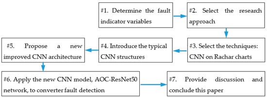
Figure 1.
The research workflow diagram.
In view of the overall process as discussed above, the remainder of this paper is organized as follows: Section 2 gives a brief introduction to the generation of radar charts; Section 3 presents deep learning network principles; Section 4 describes the improved convolutional neural network; Section 5 discusses the fault detection of the wind turbine power converter using the convolutional neural network models with a comparison of the model performance; Section 6 provides a brief discussion, and Section 7 concludes the paper and indicates future research directions.
2. Generation of Radar Chart
The radar chart analysis method is a multivariate comparative analysis based on the graphics on the similar navigation radar screen.
2.1. Radar Chart Introduction
A radar chart is a graph that shows multiple quantitative parameter value changes along different axes starting from the same original point. It can be used to describe multivariate data. The relative position and angle of the radar chart axis are usually the undefined information. It is often called a network chart, spider chart, star chart, Kiviat chart or irregular polygon. It is a typical evaluation method based on graphically comprehensive analysis. It is, therefore, suitable for the comprehensive analysis and comparison of multiple factors. It can vividly and intuitively reflect the comprehensive attributes of the evaluation target. Its advantages are that it is intuitive, vivid and easy to operate [51].
The radar chart shows the visual expression of numerical data from the perspective of “face thinking”, and converts the information in the high-dimensional invisible space into intuitive planar information. Radar charts are widely used in scientific research and industrial fields for data visualization and graphical representation for effectively displaying multiple variables [52,53,54,55].
Before drawing a graph, the data need to be standardized, usually in the interval [0,1]. If there are m numerical data with n-dimensional features, each line in the figure represents a one-dimensional variable in the process of drawing, and there are n in total. They intersect at the center of the circle. Connect the points corresponding to each variable value in order to form a closed n polygon. Finally, m data samples can be represented as m two-dimensional n polygons so that the original numerical data are represented by an image.
2.2. Radar Chart Drawing
The SCADA system data of wind turbines were collected from two-year operation data of 27 wind turbines in a wind farm in Hebei Province, China, which was put into operation in 2012. Before proceeding to draw radar charts, the fault indicator variables must be determined. The function of the converter in the operation control of a wind turbine is illustrated in Figure 2. The converter plays a role to make sure that the output power complies with the requirements of grid. It ensures that the output voltage is in a threshold range and the current frequency is in accordance with the grid. The output power of the generator is under control through adjusting the blade angle by a pitch control system. According to an investigation and analysis, the grid-side converter voltage, generator torque set-point, active and reactive power, wind speed, turbine rotor position and generator rotor speed are selected as the fault indicators of the converter. Wind speed is measured by wind sensor standing on the top and rear of wind turbine nacelle. Turbine rotor position and generator rotor speed are measured, and the other parameter values are recorded in wind turbine operation.
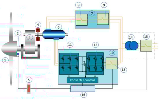
Figure 2.
Schematic of wind turbine control system diagram. (1) Rotor; (2) main shaft; (3) gearbox; (4) brake system; (5) pitch control system; (6) generator; (7) power control to the grid; (8) low voltage switchgear; (9) low voltage switchgear; (10) converter system; (11) generator side converter; (12) grid side converter; (13) on/off switch control; (14) transformer; (15) high voltage switchgear; (16) wind turbine controller.
With the SCADA system data, one can extract the data 30 min, 3 h, 24 h, 7 days or 15 days ahead of occurrence of failures and put the data into a design Excel table. Table 1 shows an example of the fault indicator variable data which are 24 h ahead of a converter failure. Each table, like Table 1, has 181 rows of data, and a total of 100 sets of data were extracted for study in this paper; the extracted normal operation data were in the same sample size as the failure data set.

Table 1.
Sample of fault indicator variable data of converter.
The specific steps for drawing a radar chart in this paper are as follows:
The first step is to select the wind speed index as the drawing reference;
The second step is to normalize the fault indicator variable values representing the converter operation condition status;
Step 3 is to collect all fault indicator variable values with a determined wind speed, and draw the 7 indicator variable values on a radar chart;
Step 4 is to draw a closed heptagon through the 7 points on the 7 axes representing the seven fault indicator variables. It is noted that the closed area defines the size of the image converted later.
The radar charts generated are shown in Figure 3 below. The numbers 1–7 in the figure represent the 7 fault indicator variables, respectively. Through drawing the graphs, the changes of the fault indicator variable values and the correlation between the fault indicator variables can be intuitively reflected. Figure 3a shows radar charts of the fault indicator variables data under normal operation of the converter; Figure 3b presents radar charts of the fault indicator variables data under faulty operation status of the converter.
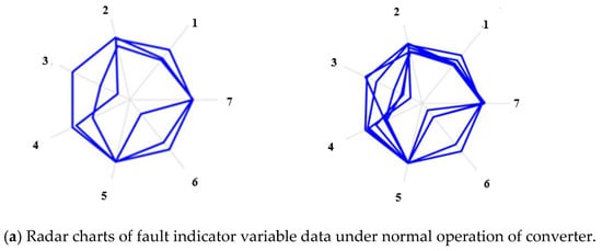
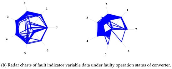
Figure 3.
Radar charts covering the fault features. (1) Wind speed; (2) turbine rotor position; (3) active power; (4) reactive power; (5) generator rotor speed; (6) grid side converter voltage; (7) generator torque set-point.
In Figure 3a, the charts were plotted corresponding to the wind speeds of 3.1 and 6.4 m/s, respectively. In the case of normal operation of the converter, the fault indicator variables data do not change much and are relatively stable. Although the amount of data is large, the number of curves shown in the graph is relatively small because of the phenomenon of data overlap, and the graph is relatively regular. In Figure 3b, the charts were plotted under the operation condition with wind speeds of 4.3 and 6.5 m/s, respectively. In the case of faulty status of the converter in operation, the fault indicator variables data change remarkably, resulting in poor regularity of the graph and irregular lines. When the system fails, some fault indicator variable data appear to be 0, such as the power data, so that incomplete graphics are observed in the radar chart. It can be seen from the figure that although there is a certain overlap in the radar chart of the fault indicator variables data, there is still a big difference from the radar charts drawn by using the normal operation data.
3. Deep Learning Network Principles
3.1. ResNet50 Convolutional Neural Network
Deep learning is an important research direction in the field of machine learning. Its introduction to machine learning makes it closer to artificial intelligence. The convolutional neural network is a deep neural network model that includes convolution. Its core process is to train and learn from a large amount of sample data through multiple iterations to extract the deep feature expression of the sample data, and finally predict the sample data according to different required tasks [56].
As the number of layers in the deep learning network increases, features of different layers can be extracted. The more abstract the feature expression, the richer the semantic information. However, as the number of original network layers in deep learning simply increases, it will cause gradients to disappear or become extremely large. The traditional method to solve this problem is generally to use reasonable weight initialization and regularization, but the implementation of the method will bring new problems of network performance degradation [57]. ResNet is a residual learning framework that can improve the performance of the network under the premise of increasing depth. The basic residual unit structure diagram of ResNet is shown in Figure 4 [58].
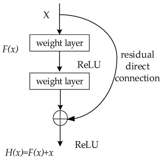
Figure 4.
Basic residual unit structure diagram [58].
If the back layer of the deep network is an identity mapping, the model can be degenerated into a shallow network. However, it is more difficult to directly use some layers to fit potential identity mapping functions, such as H(x) = x. Therefore, the network is designed as , and the problem is transformed into learning a residual function F(x) = H(x) − x. When F(x) = 0, it constitutes an identity mapping H(x) = x, so that it is easier to implement residual fitting.
In summary, the residual network structure was chosen for this paper to increase the network depth to improve the performance and accuracy of the network, and the residual structure can solve the problem of the disappearance of the gradient caused by the increase in the network depth.
The common residual network models are ResNet18, ResNet50 and ResNet101. As the number of layers increases, the amount of network calculation also increases [15,59]. By considering the calculation speed and the fault detection accuracy of the network employed, the ResNet50 structure is selected as the backbone network, and the residual unit adopts a three-layer bottleneck layer design as shown in Figure 5.
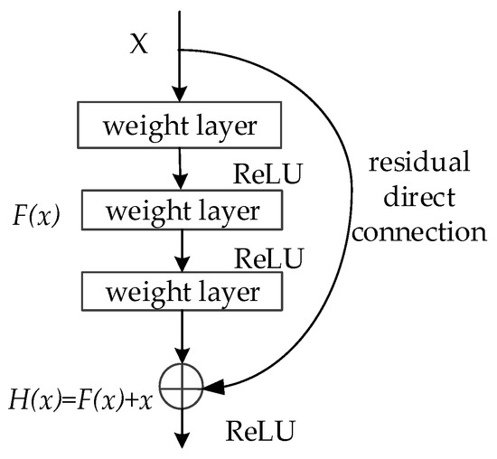
Figure 5.
Structure chart of three-layer bottleneck layer residual unit.
3.2. Oct–ResNet50 Convolutional Neural Network
Chen et al. [60] proposed a novel Octave Convolution (OctConv) operation applied to convolutional neural networks (CNNs). OctConv is designed as a single, generic, plug-and-play convolution unit that can directly replace the original convolution without the need to adjust the network architecture [60]. OctConv is dedicated to reducing the spatial redundancy in CNNs and aims to replace the ordinary convolution operations without adjusting the backbone CNN architecture. It is confirmed that OctConv has superiority over the ordinary convolution methods in improving efficiency and performance of CNN models [60].
- Idea for OctConv
The idea for OctConv is to understand the image from the perspective of the frequency domain. To view an image from the perspective of spatial domain, it can be generally represented by a c × H × W matrix where H and W denote the spatial dimensions and c is the number of feature maps or channels. Each position in the matrix corresponds to a value of [0, 255]. From the perspective of the frequency domain, the image can be decomposed into low spatial frequency components (low frequency domain) that describe smoothly changing structures and high spatial frequency components (high frequency domain) that describe the fast-changing fine details. It can effectively process the corresponding low-frequency and high-frequency components, and can also achieve effective interfrequency communication.
OctConv defines the feature map after the “downsampling” operation as the “low frequency domain”, while the original size feature map without downsampling is defined as the “high frequency domain”. After the above operations, the size of the feature map is reduced due to downsampling, thereby reducing the computation amount of OctConv. In addition, because the network has different scales of information (two frequency domains) and the two scales of the information are aggregated after the convolution is completed, the performance of OctConv is improved.
- 2.
- OctConv Principle
OctConv is a combination of downsampling and upsampling operation, as shown in Figure 6, where the green arrows represent the operation of information updates; the red arrows facilitate information exchange between the two frequencies; and X and Y are the input and output tensors, respectively. Between the input and output, it is the convolution process.
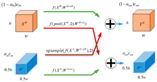
Figure 6.
OctConv convolution schematic [60].
The output, Y, is expressed by:
where the format represents the convolutional update from the feature map group A to B, and denote the high- and low-frequency components of Y, respectively. Specifically, and indicate intrafrequency update, and and indicate interfrequency communication.
In order to obtain the above terms, the convolution kernel W is divided into for the convolution with the input feature maps of and , respectively. Each component can be further divided into two parts (within frequency part and between frequencies part), namely, and .
The main work of OctConv is to split the original convolution operation into four operations, and the input processed by three of these four operations is half the height and width of the original feature map. Therefore, the amount of computation is reduced.
Using average pooling for downsampling, the output is:
where, represents the convolution with the parameter, W; represents the average pooling operation with the kernel size and the step size, k; and is the upsampling operation with the factor through the nearest interpolation.
The four parallel lines in Figure 4 correspond to the four terms in Equation (1). The two green paths, namely, the first and the fourth, correspond to the information update of the high-frequency and low-frequency feature maps, respectively; the two red paths play the role of information exchange between the two frequency domains.
- 3.
- OctConv Operation
The number of feature map channels is divided into high frequency and low frequency according to the preset coefficient, am. The width and height of the low frequency part are reduced to half of the original. OctConv performs the following operations:
- (1)
- The high frequency part is directly convolved through , that is, high frequency to high frequency convolution; the number of output channels is .
- (2)
- The high-frequency part is first downsampled and then convolved. The downsampling is by and then , that is, the convolution from high-frequency to low-frequency, and the number of output channels is .
- (3)
- The low frequency part is directly convolved and then upsampled, is the convolution from low frequency to high frequency and the number of output channels is .
- (4)
- The low frequency part directly convolves in , that is, the low frequency to the low frequency convolution; the number of output channels is .
The above operations are followed by the information aggregation process, i.e., the results from the first and third path are added by bit, and it is the same for the output results from the second and fourth path; see Figure 6.
4. Analysis of Principles of Improved Convolutional Neural Network Based on Frequency Domain Features
OctConv is suitable for the majority of existing trunk network structures, such as ResNet and MobileNet, which can bring performance improvement while reducing the amount of computation of existing models and is validated in ImageNet Classification tasks.
However, this paper finds that there are two deficiencies in the OctConv structure. The first is the asymmetry of information caused by the asymmetry of the upper- and lower-sampling methods; the second is that OctConv adopts the way that the two frequency domain features are directly added together to ensure the information interaction between the high- and low-frequency domains; however, it is likely to destroy the original characteristics of the features at the high frequency domain and the low frequency domain.
Therefore, this paper makes improvement to the OCtConv structure to overcome the above two deficiencies, and proposes the structure of Attention Octave Convolution.
4.1. Improvement in Sampling Methods
OctConv’s downsampling uses the average pooling method. When conducting upsampling, the same pixel values are copied in the upsampling step size, and the step size is 2 for both the downsampling and the upsampling, as shown in Figure 7.
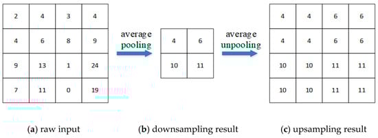
Figure 7.
OctConv sampling principle.
The OctConv sampling method will cause information asymmetry. In view of this problem, this paper proposes to change OctConv’s existing sampling method as shown below.
Replace the original OctConv downsampling with max pooling and the original upsampling with the form of max unpooling as shown in Figure 8 below.
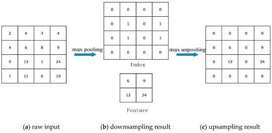
Figure 8.
Improved OctConv sampling principle.
The improved downsampling process outputs the sampling index in addition to the sampled feature map. During the sampling process, the feature map can be restored according to the corresponding index, and its other positions can be made up to 0.
Compared to average pooling, the max pooling operation can better preserve the local maximum points in the feature graph where the local maximum points generally characterize the information of the edges or corners of the image. In addition, the max pooling operation can produce a corresponding sampling index which provides a basis for subsequent upsampling operations, thereby achieving symmetry in the downsampling and upsampling processes.
In summary, max pooling and max unpooling are better suited for sampling tasks in OctConv. Because of the number of channels in the index, this paper adjusts the operation from the low frequency domain to the high frequency domain in OctConv, that is, the max unpooling operation is carried out first, followed by the convolution operation, in order to restore the feature graph in the upper sample.
4.2. Add a Branch of the Self-Attention Mechanism
OctConv transforms an existing backbone network into a two-stream format, i.e., high-frequency and low-frequency domains. At the same time, in order to ensure the two-stream information interaction, the information at the two frequency domains is directly added to the corresponding position and then reverted to the form of two streams at the end of each OctConv module, as shown in the following procedure.
where, and are the information after convolution transforms within their respective frequency domains, and are the information after the convolution transforms across the frequency domains and the addition of the corresponding positions of the feature graph can ensure the information interaction within the two frequency domains, but the information in and may destroy the information of and in the original frequency domain.
In summary, this paper introduces an Attention mechanism, an adaptive control of the information interaction process in the OctConv module. This is to control and feature diagram information to be added to the feature diagrams of and .
The specific operation is to multiply each channel in and by its corresponding coefficient to achieve the effect of scaling the feature map, as shown in Figure 7. The size of the input feature map X in Figure 9 is , and the layer in the right branch is responsible for the Attention task. The specific implementation process is as follows: First, the input feature map X is subjected to global average pooling, and the output size becomes 1 × 1 × c. Second, the feature extraction is achieved through two fully connected layers, and , successively. The output of the layer is the feature vector with 1 × 1 × c/16 dimensions, and it is activated by ReLU. The purpose of is to reduce the number of channels for reducing the number of parameters and computation. The output of the layer is the feature vector with dimensions, which serves the purpose of the further extraction of features and re-upgrading the number of channels from to , keeping it consistent with the original input. In order to prevent the output characteristics from being destroyed, the output of the layer is no longer activated by ReLU. Finally, the sigmoid function is used to compress the features of each channel in the output feature vector to the range of [0,1]. After the original input X passes through the attention branch, the output feature vector becomes dimensions. The feature vector is multiplied by the original input X channel by channel, and the result is used as the new output of .
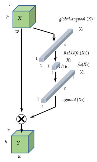
Figure 9.
The branch structure diagram of self-attention mechanism.
The above structure is introduced into and branches, and the output of the two branches is controlled by self-supervision. When and are not suitable for fusion with the original and , the scale coefficient will approach 0, and, on the contrary, it will approach 1.
The self-attention mechanism proposed in this paper has the following characteristics:
- (1)
- All layers in the Attention branch are differentiable, that is, they can directly participate in the network end-to-end training task.
- (2)
- After the output of the Attention branch passes the sigmoid threshold, the output range is limited to [0,1], which ensures that the value in the original feature will not be excessively scaled.
- (3)
- When the model performs a prediction task, the output of the Attention branch is not a fixed value but is determined by the original input, that is, it responds differently to different inputs.
The structure of AOctConv proposed in this paper is shown in Figure 10, where f(XH; WH→H) and f(XL; WL→L) represent high frequency to high frequency and low frequency to low frequency convolution, respectively; max pool(XH, 2) denotes the maximum pooling operation; max unpool(XL, 2) is a function which applies the maximum unpooling operation and upsamples the spatial dimensions of the input data; ψ is an upsampling operation based on the index; and is a function of the information represented by or . When max unpool(XL, 2) performs upsampling, the index generated by downsampling is used for max unpooling, and the Attention branch added by and branches is represented by . The branches represented by f(XH; WH→H) and f(XL; WL→L) keep the original operation without change.
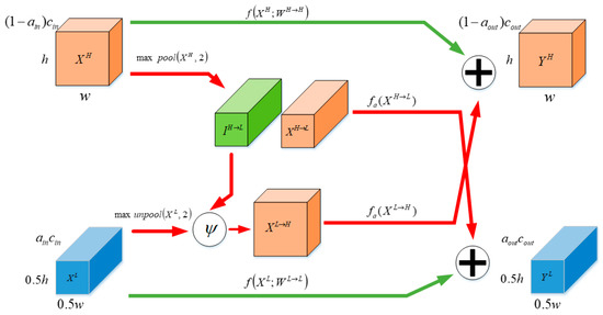
Figure 10.
AOctConv module.
4.3. Comparison of Three Network Structures
The overall structures of ResNet50, Oct–ResNet50 and AOC–ResNet50 networks are shown in Table 2 below.
Table 2.
Comparison of three network structures.
The image input size is 224 × 224, and the number of output categories is 2. It should be noted that when calculating the amount of computation, the computation at the fully connected layer and the convolutional layer includes the addition operation and also includes the computation consumption at other layers, such as the pooling layer, the BN layer and the ReLU layer.
In a forward process, ResNet50 needs 4.11 GFLOPs of computation, and the parameter number is 23.51 M; Oct–ResNet50 needs 2.38 GFLOPs of computation, and the parameter number is 23.51 M; AOC–ResNet50 needs 2.42 GFLOPs of computation, and parameter number is 23.53 M. Through the comparison of network parameters, Oct–ResNet50 has a significant reduction in the amount of computation, which is reduced by 42.09%, and the number of parameters does not change by comparing with the ResNet50 network. Compared with Oct–ResNet50, the improved algorithm of AOC–ResNet50 has a computation increase of 0.04 G FLOPs, accounting for 0.84% of the original computation and a parameter increase of 0.02 M Params, accounting for 0.08% of the original parameters, a slight increase. However, compared with the ResNet50 network, AOC–ResNet50 still has a significant decrease in the amount of computation.
The improved algorithm of AOC–ResNet50 solves the problem of information asymmetry caused by the asymmetric sampling method in the original OctConv structure and the damage to the original features in the high and low frequency domains by the OctConv structure, and improves the accuracy of fault detection as demonstrated in the following section.
5. Wind Turbine Power Converter Fault Detection
This article applied the improved AOctConv structure to the ResNet50 backbone network, and proposes the AOC–ResNet50 network. Based on the radar charts of converter fault indicator variables data which occurred 24 h, 3 days, 7 days and 15 days before a failure, this paper used ResNet50, Oct–ResNet50 and AOC–ResNet50 network structures to train and validate the fault detection models. After validation, each model’s structure was determined including the weight of each link. Then, the models were applied to fault detection using SCADA system data. The fault detection performance indices were compared among these models using the test sample data. The effectiveness of these network models was then verified.
- (1)
- Sample data
As a pure electric component, the wind turbine converter has a high frequency of failures due to frequent starting and braking. For the faulty operation data, the data that occurred 24 h, 3, 7 and 15 days before the occurrence of a converter failure were extracted, the sampling frequency was every 10 min and 100 sets of the data were collected during each fault time period (each fault time period refers to 1, 3, 7 and 15 days, respectively).
The normal operation data are the data when the system has no fault, and the extracted quantity is the same as the failure operation data. In each group of the data collected, the normal operation data dimensions were 14,400 × 7; and corresponding to each fault time period, the faulty operation data dimensions were 14,400 × 7 as well. Taking the wind speed as the reference index, after normalization of each fault indicator variable values, the radar charts were drawn. Corresponding to each fault time period, 17,001 radar charts representing the normal operation of converter and 17,001 radar charts corresponding to the faulty operation status of the converters were generated, totaling 34,002. Among them, 11,900 normal and faulty status radar charts were selected for training, and 5101 normal and faulty status radar charts were selected for testing.
- (2)
- Implementation of the training and testing method
In order to adapt to the task of fault detection, the output dimension of the final fully connected layer of the AOC–ResNet50 network was set as 2 in this paper. In the training process, the original radar image size of 256 × 256 pixels was first scaled to the universal size 224 × 224 pixels, and then the whitening operation was performed after expansion to three channels, and no other data augmentation operations were performed. Finally, the picture was used as the input of the model training. The loss function of the task training used cross-entropy loss, batch size was 64, stochastic gradient descent (SGD) method was used for optimization and the training framework was Pytorch.
- (3)
- Hardware platform utilized
Training GPU: Single card RTX2080Ti.
CPU Intel(R) Xeon(R) CPU E5–2650 v4 @ 2.20GHz.
Memory: 256 G.
- (4)
- Analysis of fault detection results for converter
In order to verify the effectiveness of the proposed AOC–ResNet50 network, ResNet50, Oct–ResNet50 and AOC–ResNet50 networks were used for converter fault detection, and the fault detection results obtained are shown in Table 3, Table 4, Table 5, Table 6 and Table 7 below. In Table 3 and Table 5, TP denotes True Positive, which means that the true value is true and the detected/predicted value is true; FN is False Negative, which means that the true value is true and the detected/predicted value is false; FP is False Positive, meaning that the true value is false and the detected/predicted value is true; and TN is True Negative, which means that the true value is false and the detected/predicted value is false. In Table 4, Table 6 and Table 7, accuracy = (TP + TN)/(TP + TN + FP + FN); precision = TP/(TP + FP); recall = TP/(TP + FN); specificity = TN/(TN + FP); and negative precision = TN/(TN + FN). Table 3 and Table 4 show the fault detection results by using the models which were trained using the variables data that occurred 3 days before occurrence of converter failures. Table 5 and Table 6 present the fault detection results by using the models which were trained using the variables data which occurred 7 days before converter failures. Table 7 gives a comparison of the fault detection performance of three models developed using the AOC–ResNet50 network and trained using the variables data that occurred 3, 7 and 15 days ahead of converter failures. It is observed that the model’s performance becomes better if trained using the variables data which occurred nearer to the time of a converter failure.
Table 3.
Converter fault detection results.
Table 4.
Converter fault detection performance indices.
Table 5.
Converter fault detection results.
Table 6.
Converter fault detection performance indices.
Table 7.
Converter fault detection performance indices by AOC–ResNet50.
From the fault detection results and detection performance indices shown in Table 3, Table 4, Table 5 and Table 6, it can be observed that the AOC–ResNet50 network proposed in this paper has the best performance. Taking the results shown in Table 4 as an example, the fault detection accuracy of the AOC–ResNet50 network model is 5.48% higher than the Oct–ResNet50 model and 7.52% higher than the ResNet50 model, while other performance indices are also superior. In addition, there is no significant difference in the values of the recall rate of the three network models. It is clearly verified that the AOC–ResNet50 outperforms Oct–ResNet50 and ResNet50 in fault detection of the wind turbine converter.
In order to verify the robustness of each obtained model, the training and testing process was repeated five times. Then, the obtained models were applied to fault detection using the same data set. It was found that each model has the same performance in terms of fault detection using the same dataset. Therefore, the model’s robustness was confirmed.
6. Discussion
A data-driven approach was selected for converter fault detection using SCADA system data in this paper. It was found that the proposed CNN network, AOC–ResNet50 network model, is better than other competitive CNN network models, such as ResNet50 and Oct–ResNet50 network models, in converter fault detection using the SCADA system data. This is due to the advantage of the AOC–ResNet50 network that it avoids the information asymmetry and the damage to the original features in the high and low frequency domains in the information sampling by comparing to the OctConv structure.
Although the AOC–ResNet50 network can provide higher accuracy in fault detection, it requires a large data sample for training the model, and the detection accuracy also relies on the data quality. Another disadvantage is that the algorithm associated with the AOC–ResNet50 network is more complex and requires the developer to have a strong mathematical background to understand the network structure and very good skills in software programing.
Selection of an approach to fault detection or diagnosis depends on the available signals and data recordings. If there are direct measurement signals corresponding to a failure mode, the methods based on signal processing and analysis would be preferred. If there are no direct measurement signals but there are indirect measurement data and operation data, a data-driven approach would be selected. In this case, CNN and other neural network models can be selected for testing. In general, if it is a complex system with multiple-dimension data available including operation and condition monitoring data, the newly proposed AOC–ResNet50 network as well as other typical CNN models are recommended for trial.
In the cases where there are direct measurement signals and the data sample size is large enough, the AOC–ResNet50 network and other typical CNN models are also recommended for application. In this situation, one may carry out a comparative study of the model performance by making a comparison between the CNN models and the models developed using signal processing and analysis methods, e.g., to detect and diagnose bearing faults for failure prediction [61].
7. Conclusions
In this paper, a deep learning approach was employed to develop fault detection models for wind turbine converters. The contribution of this paper includes two aspects: first, it proposes an innovative convolutional neural network structure named the AOC–ResNet50 network based on improvement of the Octave Convolution (OctConv) network by overcoming its two shortcomings; second, the AOC–ResNet50 network model is established and applied to wind turbine converter fault detection using wind turbine SCADA system data, and its effectiveness in fault detection was verified by a comparative study with other competitive CNN models including ResNet50 and Oct–ResNet50 network models.
The algorithm based on the AOC–ResNet50 network first replaces the downsampling and upsampling in the original OctConv structure with max pooling and max unpooling methods, and then introduces the branch of self-attention when the high-frequency domain features are fused to the low-frequency domain features, and the low-frequency domain features are fused to the high-frequency domain features. It controls the fusion process of the two frequency domains. After the AOC–ResNet50 network is developed, it is employed to extract the features of radar charts generated using the seven fault indicator variables data extracted from the wind turbine SCADA system for fault detection of the wind turbine converter. The fault detection performance indices were compared with the ResNet50 and Oct–ResNet50 networks to verify the effectiveness of the improved network. It was found that the fault detection performance using the AOC–ResNet50 network is superior to the ResNet50 and Oct–ResNet50 networks. The fault detection accuracy of AOC–ResNet50 network model can be up to 98.0%, which is 5.48% higher than Oct–ResNet50 and 7.52% higher than the ResNet50 model based on the radar charts generated using the fault indicator variables data that occurred 3 days ahead of converter failures. In the next step of our research work, the AOC–ResNet50 network will be applied to wind turbine converter failure prediction using fault indicator variables data that occur at different time periods before a failure occurs. At the same time, the AOC–ResNet50 network will be applied to fault detection and failure prediction for other wind turbine components.
Author Contributions
Methodology, C.X. and Z.L.; software, C.X. and X.Z.; validation, C.X., T.Z. and X.Z; formal analysis, C.X., T.Z. and X.Z.; investigation, C.X., X.Z. and Z.L.; data curation, X.Z. and C.X.; writing—original draft preparation, C.X. and T.Z. and X.Z.; writing—review and editing, T.Z. and C.X.; supervision, Z.L. and T.Z. All authors have read and agreed to the published version of the manuscript.
Funding
This work was partially supported by the National Natural Science Foundation of China (61703135; 61773151; 51577008); Hebei Natural Science Foundation (F2015202231); Youth Fund of Hebei Education Department (QN2019122); Key Project of North China Institute of Aerospace Engineering (ZD202003); The Excellent Going Abroad Experts Training Program in Hebei Province.
Institutional Review Board Statement
Not applicable.
Informed Consent Statement
Not applicable.
Data Availability Statement
The data presented in this study are available on request from the corresponding author. The data are not publicly available due to privacy.
Acknowledgments
The wind turbine operation data were collected from a wind farm in Hebei Province, China. The authors are grateful to the wind farm manager and engineers for their kind support.
Conflicts of Interest
The authors declare no conflict of interest.
References
- WWEA. Available online: https://wwindea.org/blog/category/statistics/ (accessed on 20 November 2020).
- Zhao, L.; Yang, H. Optimal control of grid-connected converter under asymmetrical grid voltage fault. Micro Motors. 2018, 5, 52–58. [Google Scholar]
- Witczak, M.; Rotondo, D.; Puig, V.; Nejjari, F.; Pazera, M. Fault estimation of wind turbines using adaptive and parameter estimation schemes. Int. J. Adapt. Control Signal Process. 2018, 32, 549–567. [Google Scholar] [CrossRef]
- Tutivén, C.; Vidal, Y.; Acho, L.; Rodellar, J. A fault detection method for pitch actuators faults in wind turbines. Renew. Energy Power Qual. J. 2015, 1, 698–703. [Google Scholar]
- Wu, D.; Liu, W. A new fault diagnosis approach for the pitch system of wind turbines. Adv. Mech. Eng. 2017, 9, 1–9. [Google Scholar] [CrossRef]
- Qiao, W.; Lu, D.G. A survey on wind turbine condition monitoring and fault diagnosis−Part II: Signals and signal processing methods. IEEE Trans. Ind. Electron. 2015, 62, 6546–6557. [Google Scholar] [CrossRef]
- Zhang, Z.Y. Automatic fault prediction of wind turbine main bearing based on SCADA data and artificial neural network. Open J. Appl. Sci. 2018, 8, 211–225. [Google Scholar] [CrossRef]
- Simani, S.; Farsoni, S.; Castaldi, P. Data-driven techniques for the fault diagnosis of a wind turbine benchmark. Int. J. Appl. Math. Comput. Sci. 2018, 28, 247–268. [Google Scholar] [CrossRef]
- Bi, R.; Zhou, C.K.; Hepburn, D.M. Detection and classification of faults in pitch-regulated wind turbine generators using normal behaviour models based on performance curves. Renew. Energy 2017, 105, 674–688. [Google Scholar] [CrossRef]
- Pashazadeh, V.; Salmasi, F.R.; Araabi, B.N. Data driven sensor and actuator fault detection and isolation in wind turbine using classifier fusion. Renew. Energy 2018, 116, 99–106. [Google Scholar] [CrossRef]
- Zhao, H.S.; Liu, H.H.; Hu, W.J.; Yan, X. Anomaly detection and fault analysis of wind turbine components based on deep learning network. Renew. Energy 2018, 127, 825–834. [Google Scholar] [CrossRef]
- Helbing, G.; Ritter, M. Deep Learning for fault detection in wind turbines. Renew. Sustain. Energy Rev. 2018, 98, 189–198. [Google Scholar] [CrossRef]
- Teng, W.; Cheng, H.; Ding, X.; Liu, Y.; Ma, Z.; Mu, H. DNN-based approach for fault detection in a direct drive wind turbine. IET Renew. Power Gener. 2018, 12, 1164–1171. [Google Scholar] [CrossRef]
- Tautz-Weinert, J.; Watson, S.J. Using SCADA data for wind turbine condition monitoring—A review. IET Renew. Power Gener. 2017, 11, 382–394. [Google Scholar] [CrossRef]
- Shen, Y.X.; Zhou, W.J.; Ji, Z.C.; Wu, D.H. Fault diagnosis of converter used in wind power generation based on wavelet packet analysis and SVM. Acta Energ. Sol. Sin. 2015, 36, 785–791. [Google Scholar]
- Santos, P.; Villa, L.F.; Reñones, A.; Bustillo, A.; Maudes, J. An SVM-based solution for fault detection in wind turbines. Sensors 2015, 15, 5627–5648. [Google Scholar] [CrossRef]
- Zhang, P.J.; Lu, D.L. A survey of condition monitoring and fault diagnosis toward integrated O&M for wind turbines. Energies 2019, 12, 2801. [Google Scholar] [CrossRef]
- Xiao, C.; Liu, Z.J.; Zhang, T.L.; Zhang, L. On fault prediction for wind turbine pitch system using radar chart and support vector machine approach. Energies 2019, 12, 2693. [Google Scholar] [CrossRef]
- Kavaz, A.G.; Barutcu, B. Fault detection of wind turbine sensors using artificial neural networks. J. Sens. 2018, 5628429. [Google Scholar] [CrossRef]
- Zhang, Z.Y.; Wang, K.S. Wind turbine fault detection based on SCADA data analysis using ANN. Adv. Manuf. 2014, 2, 70–78. [Google Scholar] [CrossRef]
- Kim, K.; Parthasarathy, G.; Uluyol, O.; Foslien, W.; Shuangwen, S.; Fleming, P. Use of SCADA data for failure detection in wind turbines. In Proceedings of the 2011 Energy Sustainability Conference and Fuel Cell Conference, Washington, DC, USA, 7–10 August 2011. [Google Scholar]
- Joshuva, A.; Sugumaran, V. Fault diagnostic methods for wind turbine: A review. ARPN J. Eng. Appl. Sci. 2016, 11, 4654–4668. [Google Scholar]
- Maldonado-Correa, J.; Martín-Martínnez, S.; Artigao, E.; Gómez-Lázaro, E. Using SCADA data for wind turbine condition monitoring: A systematic literature review. Energies 2020, 13, 3132. [Google Scholar] [CrossRef]
- Chen, L.T.; Xu, G.H.; Zhang, Q.; Zhang, X. Learning deep representation of imbalanced SCADA data for fault detection of wind turbines. Measurement 2019, 139, 370–379. [Google Scholar] [CrossRef]
- Li, M.; Wang, S.X.; Fang, S.X.; Zhao, J. Anomaly detection of wind turbines based on deep small-world neural network. Appl. Sci. 2020, 10, 1243. [Google Scholar] [CrossRef]
- Stetco, A.; Dinmohammadi, D.; Zhao, X.Y.; Robu, V.; Flynn, D.; Barnes, M.; Keane, J.; Nenadic, G. Machine learning methods for wind turbine condition monitoring: A review. Renew. Energy 2019, 133, 620–635. [Google Scholar] [CrossRef]
- Jiang, G.; He, H.; Yan, J.; Xie, P. Multiscale convolutional neural networks for fault diagnosis of wind turbine gearbox. IEEE Trans. Ind. Electron. 2019, 66, 3196–3207. [Google Scholar] [CrossRef]
- Wang, Z.J.; Zhen, L.K.; Du, W.H. A novel method for intelligent fault diagnosis of bearing based on Capsule neural network. Complexity 2019, 6943234. [Google Scholar] [CrossRef]
- Chatterjee, J.; Dethlefs, N. Deep learning with knowledge transfer for explainable anomaly prediction in wind turbines. Wind Energy 2020, 23, 1693–1710. [Google Scholar] [CrossRef]
- Kong, Y.; Wang, T.Y.; Feng, Z.P.; Chu, F. Discriminative dictionary learning based sparse representation classification for intelligent fault identification of planet bearings in wind turbine. Renew. Energy 2020, 152, 754–769. [Google Scholar] [CrossRef]
- Chen, P.; Li, Y.; Wang, K.S.; Zuo, M.J.; Heyns, P.S.; Baggeröhr, S. A threshold self-setting condition monitoring scheme for wind turbine generator bearings based on deep convolutional generative adversarial networks. Measurement 2021, 167, 108234. [Google Scholar] [CrossRef]
- Saufi, S.R.; Ahmad, Z.A.B.; Leong, M.S.; Lim, H.M. Gearbox fault diagnosis using a deep learning model with limited data sample. IEEE Trans. Ind. Inform. 2020, 16, 6263–6271. [Google Scholar] [CrossRef]
- An, Q.T.; Sun, L.Z.; Zhao, K. Current residual vector-based open-switch fault diagnosis of inverters in PMSM drive systems. IEEE Trans. Power Electron. 2015, 30, 2814–2827. [Google Scholar] [CrossRef]
- Baygildina, E.; Smirnova, L.; Juntunen, R.; Murashko, K.; Mityakov, A.V.; Kuisma, M.; Sapozhnikov, S.Z. Condition monitoring of wind power converters using heat flux sensor. Int. Rev. Electr. Eng. 2016, 11, 239–246. [Google Scholar] [CrossRef]
- Hackl, C.M.; Pecha, U.; Schechner, K. Modeling and control of permanent-magnet synchronous generators under open-switch converter faults. IEEE Trans. Power Electron. 2019, 34, 2966–2979. [Google Scholar] [CrossRef]
- Mendes, A.M.S.; Abadi, M.B.; Cru, S.M.A. Fault diagnostic algorithm for three-level neutral point clamped AC motor drives, based on the average current Park’s vector. IET Power Electron. 2014, 7, 1127–1137. [Google Scholar] [CrossRef]
- Zhao, H.; Cheng, L. Open-circuit faults diagnosis in back-to-back converters of DF wind turbine. IET Renew. Power Gener. 2017, 11, 417–424. [Google Scholar] [CrossRef]
- Huang, K.Y.; Liu, J.J.; Huang, S.D. Converters open-circuit fault-diagnosis methods research for direct-driven permanent magnet wind power system. Trans. China Electrotech. Soc. 2015, 30, 129–136. [Google Scholar]
- Qiu, Y.; Jiang, H.; Feng, Y.; Cao, M.; Zhao, Y.; Li, D. A new fault diagnosis algorithm for PMSG wind turbine power converters under variable wind speed conditions. Energies 2016, 9, 548. [Google Scholar] [CrossRef]
- Choi, C.; Lee, W. Design and evaluation of voltage measurement-based sectoral diagnosis method for inverter open switch faults of permanent magnet synchronous motor drives. IET Electr. Power Appl. 2012, 6, 526–532. [Google Scholar] [CrossRef]
- Freire, N.M.A.; Estima, J.O.; Cardoso, A.J.M. A voltage-based approach without extra hardware for open-circuit fault diagnosis in closed-loop PWM AC regenerative drives. IEEE Trans. Ind. Electron. 2014, 61, 4960–4970. [Google Scholar] [CrossRef]
- Zhang, H.X.; Tan, Y.H.; Zhou, Y. Characteristic analysis for permanent magnet synchronous generator wind power systems during converter faults. Proc. CSEE 2018, 38, 7045–7051. (In Chinese) [Google Scholar]
- Hang, J.; Zhang, J.Z.; Cheng, M. Fault diagnosis of open-circuit faults in converters of direct-driven permanent magnet wind power generation systems based on line voltage errors. Proc. CSEE. 2017, 37, 2933–2943. (In Chinese) [Google Scholar]
- Wang, H.Y.; Pei, X.J.; Wu, Y.H. Switch fault diagnosis method for series-parallel forward DC-DC converter system. IEEE Trans. Ind. Electron. 2019, 66, 4684–4695. [Google Scholar] [CrossRef]
- Potamianos, P.G.; Mitronikas, E.D.; Safacas, A.N. Open-circuit fault diagnosis for matrix converter drives and remedial operation using carrier-based modulation methods. IEEE Trans. Ind. Electron. 2014, 61, 531–545. [Google Scholar] [CrossRef]
- Xue, Z.Y.; Xiahou, K.S.; Li, M.S. Diagnosis of multiple open-circuit switch faults based on Long Short-Term Memory Network for DFIG-based wind turbine systems. IEEE J. Emerg. Sel. Top. Power Electron. 2020, 8, 2600–2610. [Google Scholar] [CrossRef]
- Kouadri, A.; Hajji, M.; Harkat, M.-F.; Abodayeh, K.; Mansouri, M.; Nounou, H.; Nounou, M. Hidden Markov model based principal component analysis for intelligent fault diagnosis of wind energy converter systems. Renew. Energy 2020, 150, 598–606. [Google Scholar] [CrossRef]
- Zheng, X.X.; Peng, P. Fault diagnosis of wind power converters based on compressed sensing theory and weight constrained AdaBoost-SVM. J. Power Electron. 2019, 19, 443–453. [Google Scholar]
- Liu, Z.J.; Xiao, C.; Zhang, T.L.; Zhang, X. Research fault detection for three types of wind turbine subsystems using machine learning. Energies 2020, 13, 460. [Google Scholar] [CrossRef]
- SyncedReview. Upgrading CNN with OctConv. 19 April 2019. Available online: https://medium.com/syncedreview/upgrading-cnn-with-octconv-5ed9770759be (accessed on 30 November 2020).
- Tang, Z.Y. Comprehensive Evaluation of Green Building Design Schemes; Chang’an University: Xi’an, China, July 2014. [Google Scholar]
- Joan Saary, M. Radar plots: A useful way for presenting multivariate health care data. J. Clin. Epidemiol. 2008, 61, 311–317. [Google Scholar] [CrossRef]
- Porter, M.M.; Niksiar, P. Multidimensional mechanics: Performance mapping of natural biological systems using permutated radar charts. PLoS ONE 2018, 13, e0204309. [Google Scholar] [CrossRef]
- Zhao, W.Y.; Siegel, D.; Lee, J.; Su, L.Y. An integrated framework of drivetrain degradation assessment and fault localization for offshore wind turbines. Int. J. Progn. Health Manag. 2013, 4, 46–58. [Google Scholar]
- Zhang, H.J.; Hou, Y.Y.; Zhang, J.Y.; Qi, X.Y.; Wang, F.J. A new method for nondestructive quality evaluation of the resistance spot welding based on the radar chart method and the decision tree classifier. Int. J. Adv. Manuf. Technol. 2015, 78, 841–851. [Google Scholar] [CrossRef]
- Zagoruyko, S.; Komodakis, N. Wide residual networks. arXiv 2016, arXiv:1605.07146. [Google Scholar]
- Guo, Y.; Su, P.F.; Wu, Y.F. Object detection and location of robot based on Faster R-CNN. Huazhong Univ. Sci. Tech. 2018, 46, 55–59. [Google Scholar]
- Wang, H.; Li, X.; Liu, X.F.; Wenlong, X. Classification of breast cancer histopathological images based on ResNet50 Network. J. China Univ. Metrol. 2019, 30, 72–77. [Google Scholar]
- Miao, L.; Zhao, Y.Q.; Zeng, Y.Z.; Huang, Z.C.; Zhang, B.K.; Zou, B.J. Automatic segmentation for cell images bases on support vector machine and ellipse fitting. J. Zhejiang Univ. Eng. Sci. 2017, 51, 722–728. [Google Scholar]
- Chen, Y.P.; Fan, H.Q.; Xu, B.; Yan, Z.C.; Kalantidis, Y.; Rohrbach, M.; Yan, S.C.; Feng, J.S. Drop an Octave: Reducing spatial redundancy in convolutional neural networks with Octave convolution. In Proceedings of the 2019 IEEE/CVF International Conference on Computer Vision, Seoul, Korea, 27 October–2 November 2019; pp. 3435–3444. [Google Scholar]
- Glowacz, A. Acoustic fault analysis of three commutator motors. Mech. Syst. Signal Process. 2019, 133, 106226. [Google Scholar] [CrossRef]
Publisher’s Note: MDPI stays neutral with regard to jurisdictional claims in published maps and institutional affiliations. |
© 2021 by the authors. Licensee MDPI, Basel, Switzerland. This article is an open access article distributed under the terms and conditions of the Creative Commons Attribution (CC BY) license (http://creativecommons.org/licenses/by/4.0/).