Humidity Distribution in High-Occupancy Indoor Micro-Climates

Abstract

The general consensus among academics is that the spatio-temporal humidity distribution is more or less uniform in an indoor space. This has, for the large part, not yet been proven by an academic study; subsequently, this paper aims to demonstrate that this is not always true. The paper makes use of a validated transient CFD model, which uses the Low Reynolds Number k-$ϵ$ turbulence model. The model simulates people in a room at a constant skin temperature and emitting a constant source of humidity using source terms in the species equation. The model is eventually used to predict the implications of having a high source of humidity, in the form of occupancy, on the micro-climate’s spatio-temporal humidity distribution. The results for the high-occupancy case show that different locations experience various amounts of humid air, with a 31% difference between the lowest and highest locations. The amount of water vapor in each person’s proximity is deemed to be highly dependent on the flow of the inlet jet, with the people farthest from the jet having an overall less mass of water vapor in their proximity over the two-hour experimental period. This paper has concluded that there are, in fact, cases where the humidity non-uniformity inside an interior environment becomes substantial in situations of high occupancy. The results of this paper may be useful to improve the design of HVAC systems.

1. Introduction

1.1. Background

In developed countries, people tend to spend 90% of their lives indoors [1]. Consequently, enjoying comfortable interior spaces has, in the past couple of decades, been given high importance, both by lay people in general and by academics. This can particularly be observed in the vast amount of literature related to thermal comfort that has been produced. Thermal comfort calculates the status of thermal satisfaction in any environment, and in the past, several indices have been formulated to quantify the interior comfort, with the most prominent method being the 7-point Predicted Mean Vote–Predicted Percentage of Dissatisfied (PMV-PPD) model proposed by Fanger [2].

Interestingly, however, even though the Fanger PMV-PPD model is dependent and calculated using six variables, namely activity level, clothing insulation, air velocity, air temperature, air humidity, and mean radiant temperature [3], most of the work present in literature concentrates on the effect of ambient temperature [4] and clothing insulation [5], together with a number of studies that detail how the building envelope materials and architectural features may effect the internal thermal comfort [6]. In fact, Li et al. [7], who experimentally studied the effects of a high-humidity climate on people living in hot and humid environments, state that, even though research on thermal comfort is wide and deep, studies related to the identification of the effect of relative humidity (RH) on thermal comfort is in its infancy. This is particularly true when considering localized micro-climatic characteristics of humidity in indoor spaces. In this paper, the term micro-climate is being used to define specific indoor environmental volumes that together make up a room’s interior space. Although it is generally known that below ambient conditions of 30 $°\mathrm{C}$ and 70% RH, humidity has a negligible impact on thermal comfort, the impact of high-humidity sources on the indoor environment, or the impact on thermal comfort in indoor spaces where humidity tends to reach high levels, has not yet been assessed. Nonetheless, this study shall not concentrate on the thermal comfort aspect but on the physics of the spatio-temporal distribution of humidity in an internal environment.

1.2. Current Research on the Spatio-Temporal Distribution of Air in Interior Micro-Climates

Several studies have focused on better understanding the thermal conditions occurring in specific micro-climates. Yu et al. [8] have delved into the stratification of air in a room having an underfloor indoor air distribution system, while other studies [9] analyze the effects ventilation and turbulence have on specific micro-climates, such as draughts at working plane levels in a conditioned space. Similar studies that analyze the distribution of humidity and its effect on certain micro-climates are lacking from the academic literature.

Most of these works focus on the effect of air velocity [10] and temperature [11] on thermal comfort and human perception. Yet, very few studies have analyzed in detail the effect that humidity has on perceived thermal comfort [7]. In fact, Li et al. [7] discuss how relative humidity affects the human physiological response and the thermal perception of an indoor space. They continue to add that this effect is especially felt when the indoor temperature exceeds 30 $°\mathrm{C}$ and propose that the formula for the Standard Effective Temperature (SET) be modified to provide by including a humidity correction coefficient to take care of this deviation between theoretical and actual effective temperatures. Such declarations are also backed by the work of Tanabe and Kimura [12], which deems the PMV scale highly inaccurate at high relative humidities and, thus, fails to indicate the actual thermal comfort of a space. Zhang and Yoshino [13] investigated interior humidity levels in different Chinese cities and determined that, since some case studies have an indoor humidity less than 20% or higher than 80%, these are inadequate for residents and detrimental to their health. The study, however, assumes a constant humidity throughout the whole residence. The general consensus on this topic is that relative humidities lower than 70% do not effect the human thermophysiological response, and relative humidities higher than 70% are only deemed to be uncomfortable when the ambient temperature is higher than 30 $°\mathrm{C}$ [14]. These studies, and other similar ones [15], are all implemented at a constant humidity, and the thermal response of the test subjects is analyzed for each case. A varying humidity was not tested during such an approach.

Djamila et al. [16] present one of the most advanced works in this field in which the authors try to predict the indoor humidity and its effect on the occupants’ thermal comfort through the use of regression models carried out on actual site experiments implemented in the humid tropics of Malaysia. Saber et al. [17] then generated several CFD models for low exergy cooling techniques using different turbulence models and discovered that the SST k-$\omega$ and Reynolds stress model predictions are closer to actual in situ measurements, while the standard k-$ϵ$ model shows lower temperatures in most of the calculated points.

Mortensen et al. [18] have assessed the effect of water vapor on building materials by designing a coupled CFD-material model. Wurtz et al. [19] successfully predicted the transient humidity distribution in a room while attempting to investigate the moisture adsorbing properties of building materials. Huang et al. [20] then assessed interior micro-climates via a CFD model of a room, whose mesh was divided into some 73,000 cells. This study serves as an introduction to studies on the spatial distribution of humidity but is more aimed at the verification of a new factor that was developed to predict indoor humidity, as opposed to giving a complete picture of the spatio-temporal distribution of humidity inside the room.

1.3. Current Literature on Manikin Modeling for Use in Simulations

To better understand thermal comfort, many authors have delved into the human thermophysiology subject and have come up with several methods to model a human body. The human body can be described as a thermal machine whose fuel is food and oxygen and whose output is thermal and kinetic energy [1]. To achieve thermal comfort, the rate of the heat being generated by the body must be equal to the rate being dissipated by it [21]. The human body was first modeled by Lefevre [22] as a sphere whose core exchanges heat with the surroundings. Burton [23] then came up with the first mathematical model for the human body. These models were then improved further throughout the subsequent decades [24,25,26].

Following the above studies, researchers started to implement their findings into CFD models. The most simple model of a human being implemented in CFD is that of a single cylinder or cuboid having a total surface area similar to a typical person, such as the Dubois model [27]. Other more complicated models include multi-node models, which divides the model into layers such as skin, muscle, blood, and bones, and multi-segment models which divide the body into several parts such as the head, torso, legs, arms, etc. [28]. Kaynakli and Kilic [1] divide the human body into sixteen segments, while Gagge [29] represent it as a single segment, two-nodal, cylindrical model. One of the most influential multi-node models developed for NASA during the Apollo program is the 25-node Stolwijk model, which was used to predict the thermal response of astronauts in outer space [30]. Fiala et al. [31] constructed a model which uses 15 segments and 187 nodes.

Cook et al. [32] carried out a study on cross-ventilation in classrooms and showed that a complex CFD manikin model gave similar results to a simplified human body model. This simplified human body model was also used in the humidity spatial distribution model that was studied by Huang et al. [20]. Furthermore, a CFD case study carried out by Dixit and Gade [33] determined that Fanger’s thermal comfort model [2] is not ideal for transient problems as it is not able to account for a person’s thermoregulatory activities.

1.4. Scope and Paper Outline

There is general consensus between academics that unless humidity levels are high, humidity has a negligible impact on the indoor thermal environment. Yet there are no existing studies which confirm this, and moreover, the impact of high-humidity sources on the spatial distribution of humidity in indoor environments has not yet been fully analyzed in detail. In this context, this paper aims to understand the humidity spatio-temporal distribution in indoor environments for both low- and high-humidity sources.

The paper is divided as follows. The study first looks into the methodology used to carry out in situ test chamber experiments, followed by the approach to set up and validate a CFD model, which is then used as a predictive tool. The results showing the humidity distribution in a densely populated space are then presented and discussed.

2. Methodology

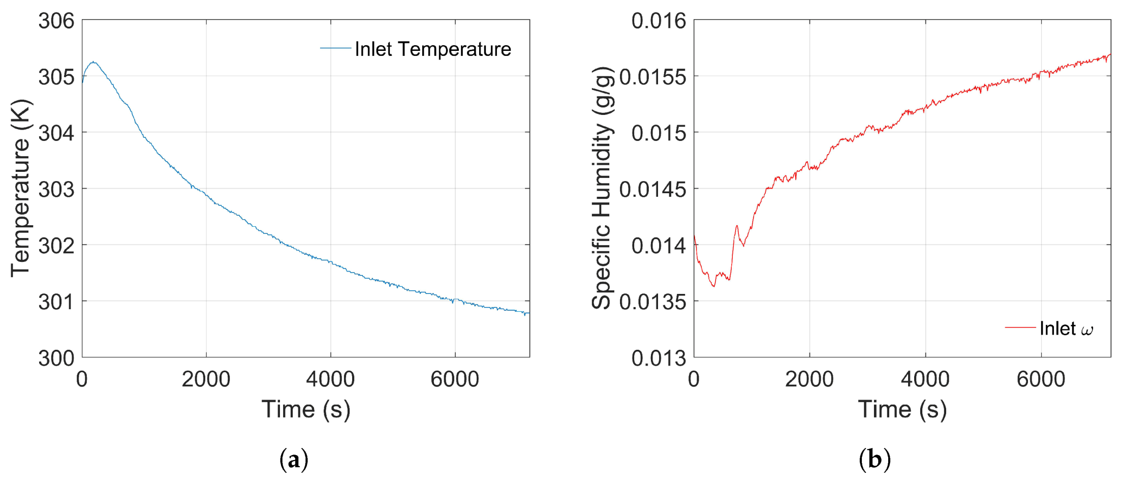
2.1. Experimental Setup

The experiments were conducted in a test chamber, shown in Figure 1, located in the Faculty for the Built Environment in a higher education institution, at basement level. The chamber was designed to replicate related studies such as that by Li et al. [7]. The room is 3 m wide, 4 m long, 3 m high, and is made of wood and expanded polystyrene. The zero coordinate (0, 0, 0) m was taken on the outlet wall, at the low level corner nearest to the jet as shown in Figure 1. The test chamber has a circular, 20 cm diameter inlet, with center at (0.19, 4.00, 2.76) m and a rectangular outlet measuring 20 cm × 20 cm, with center at (2.61, 0.00, 0.33) m. Three test subjects (TS), chosen at random, were seated in the room. The full details of the TS are tabulated in

Table 1. Test Subject Details.

	Gender	Age	Height		Weight	BMI	Clothing	Centre
			Standing	Seated			Insulation	Coordinate
			m	m		kg	clo	x	y	z
TS1	Female	32	1.69	1.21	67.5	23.6	0.57	1.21	3.39	0
TS2	Male	32	1.67	1.23	53	19	0.57	1.21	2.16	0
TS3	Male	21	1.75	1.27	72	23.5	0.57	1.21	0.68	0

.

A number of HOBO UX100-003 [34] and EL-WiFi-21CFR-TH [35] temperature and relative humidity sensors were located at distinct, significant positions in the room.

Table 2. Temperature and humidity sensors properties and locations.

Sensor	Name	Co-Ordinates			Type	Temperature		Relative Humidity		Logging
		x	y	z		Accuracy	Range	Accuracy	Range	Period
		m	m	m		$°\mathbf{C}$	$°\mathbf{C}$	%	%	s
1	Inlet	0.20	3.99	2.75	HOBO	±0.21	−20–70	±3.5	15–95	10
2	Outlet	2.61	0.01	0.44	HOBO	±0.21	−20–70	±3.5	15–95	10
3	Front	1.71	0.43	1.93	HOBO	±0.21	−20–70	±3.5	15–95	10
4	Side	2.29	2.33	1.45	21CFR	±0.30	−20–60	±2.0	0–100	60
5	Jet	0.27	2.14	2.56	21CFR	±0.30	−20–60	±2.0	0–100	60
6	Centre	1.52	2.20	2.44	HOBO	±0.21	−20–70	±3.5	15–95	10
9	Back	1.83	3.40	1.73	21CFR	±0.30	−20–60	±2.0	0–100	60

defines the sensor locations, type, accuracy, range, and logging period. To measure velocities of two points in the jet, a Thermo-Anemo-Manometer MP210 [36] coupled with SFC900GN velocity wire probes [37] was used.

Table 3. Properties and locations of velocity sensors.

Sensor	Name	Co-Ordinates			Velocity		Logging
		x	y	z	Accuracy	Range	Period
		m	m	m		m$\mathit{·}$ s${}^{-1}$	min
1	V1	0.31	2.80	2.60	±3% ±0.03 m$·$ s${}^{-1}$	0.15–30	5
2	V2	0.31	1.10	2.63	±3% ±0.03 m$·$ s${}^{-1}$	0.15–30	5

then details the probe locations, type, accuracy, range, and logging period.

The test chamber was tested for the amount of infiltration between the chamber’s interior and its exterior. Even though infiltration tests are typically carried out via a fan pressurization test as detailed by ISO 9972 [38] and ASTM E779-19 [39], other methods such as the tracer gas methods detailed by ASTM E741-11 [40] are widely used to determine the infiltration rate of an interior zone [41]. In fact, in this study, the latter method was used. The test was carried out by following the guidelines set out by Roulet and Foradini [42] and measuring the CO₂ decay in the test chamber. Using this method, it was determined that the infiltration of the room was 0.2785 m${}^3·$ h${}^{-1}$, which was much less than the 4.752 m${}^3·$ h${}^{-1}$ value suggested by ASHRAE [43] for such a test chamber. The determined infiltration value was thus considered to be very small to have a consequential impact on the modeling approach used, and, as a result, was ignored.

An inlet supplying the test chamber with a time-varying humidity jet was devised by forcing fresh air through a flat-bed non-regenerative desiccant and then humidified using both the evaporative pads and water spraying procedures. This paper does not focus on the manner in which a continuously changing humidity was obtained at the inlet (this has been done elsewhere [44]) but, alternatively, on the impact such a varying humidity, shown in Figure 2, has on the humidity profile of the room. The initial ambient conditions inside the test chamber at the start of the experiment were measured at 300.5 $\mathrm{K}$ and a specific humidity ($\omega$) of 0.015 $\mathrm{g} \mathrm{g}{}^{-1}$, equivalent to about 57.5% relative humidity. The velocity of the jet at the inlet was measured at 4 $\mathrm{m} \mathrm{s}{}^{-1}$. The inlet setup was left unchanged for the total duration of the experiment (2 h). This means that the regeneration of desiccant, which was carried out at a temperature of 250 $°\mathrm{C}$ after the end of each experiment, was not studied during this analysis.

2.2. CFD Model

A Navier–Stokes Computational Fluid Dynamics (CFD) solver was used to model and solve the problem. ANSYS Fluent version 13.0 [45], a commercial code, was selected. Due to the huge computational costs that would be required to solve a transient simulation involving 7200 s of flow time and a varying time-steps of between 1 and 10 s, twelve cores in parallel of the University of Malta supercomputing cluster, Albert [46], were used to compute this analysis. The inputs to the cluster were given using the Text User Interface (TUI). Each simulation typically lasted between two to three days.

A test chamber with the dimensions identical to the experimental one was modeled. Three seated people were modeled using the Dubois cuboid method [27] as shown in Figure 1. The cuboid dimensions were measured at 0.65 m length, 0.5 m width, and 1.2 m height. As described above, Cook et al. [32] have previously shown that modeling the human body as a complex CFD manikin model and a simplified cylindrical model has negligible impact on the properties of the surrounding micro-climate.

Given that the geometry is made up of a number of cuboids, quadrilateral mapped elements were chosen to construct the mesh. The mesh size was set to an average of 5 cm both horizontally and vertically, skewed with a bias factor of 10 towards each separating plane to capture all boundary layer flow gradients. The cells in the inlet area were refined to 5 mm to better capture the highly transient phenomena occurring in the jet. The walls near the jet were also refined to 1 cm to increase the cell gradient between the jet and these walls. On each person’s head, a layer having a height of 5 cm, divided into 10 vertical cells biased to both ends, was created. This layer was eventually used to define the humidity coming out of the seated person due to breathing. The mesh was thus made up of 1.3 million cells with a maximum skewness of 1.3 × 10⁻¹⁰ and is shown in Figure 3. The mesh was then adapted to ensure that all wall y-plus values were as small as possible (in general, below 1 but certainly not greater than 5). This demand required a substantial increase in the number of cells, but it ensured that the flow was modeled up to the wall to be able to capture wall fluxes appropriately. The resulting mapped mesh consisted of about 1.8 million cells.

A steady-state solution with around 2000 iterations was initially carried out to enable the model to capture the room’s initial conditions accurately. The model was subsequently changed to a transient one with varying time-steps. The CFD solver performed several iterations to numerically solve the energy, momentum, mass, and species equations. Natural convection effects were taken into account by setting the acceleration due to gravity at −9.81 $\mathrm{m} {\mathrm{s}}^{-2}$ in the y-direction, while the ideal gas equation was used to model the air density variation. Changes in humidity were modeled by using the Species Transport approach, defined in Equation (1). The chamber’s fluid was a mixture of air and water vapor, and the Courant Number of the model was set at 5. The turbulence model used was the Low Reynolds Number (LRNM) k-$ϵ$ model by Yang and Shih [47] as shown in Equations (2)–(5). This was determined to be the most suitable model for such a simulation.

$$\frac{\partial }{\partial t}\left(\rho Y\right)+\nabla ·\left(\rho \overrightarrow{v}Y\right)=-\nabla ·\overrightarrow{J}+R+S$$

(1)

where

• Y is the local mass fraction of the species;
• $\overrightarrow{J}$ is the diffusion flux of the species;
• R is the net rate of production of species by chemical reaction (0 in this case);
• S is the user defined source of the species (in $\mathrm{k}\mathrm{g} \mathrm{s}{}^{-1} {\mathrm{m}}^{-3}$).

$$\frac{\partial }{\partial t}\left(\rho k\right)+\frac{\partial }{\partial x_j}\left[\rho k{u}_j-\left(\mu +\frac{{\mu }_t}{{\sigma }_k}\right)\frac{\partial k}{\partial x_j}\right]=P-\rho ϵ-\rho D$$

(2)

$$\frac{\partial }{\partial t}\left(\rho ϵ\right)+\frac{\partial }{\partial x_j}\left[\rho ϵu_j-\left(\mu +\frac{{\mu }_t}{{\sigma }_{ϵ}}\right)\frac{\partial ϵ}{\partial x_j}\right]=\left(C_{ϵ1}{f}_{1}P-C_{ϵ2}{f}_2\rho ϵ\right)\frac{ϵ}{k}+\rho E$$

(3)

$${\mu }_t=C_{\mu }{f}_{\mu }\rho \frac{k^2}{ϵ}$$

(4)

$$P={\tau }_{ij}^{turb}\frac{\partial u_i}{\partial x_j}$$

(5)

where

• $C_{{ϵ}_1}$, $C_{{ϵ}_2}$, $C_{\mu }$, ${\sigma }_k$, and ${\sigma }_{ϵ}$ are model constants;
• $f_{\mu }$, $f_1$, and $f_2$ are damping functions;
• $\mu$ is the dynamic viscosity;
• D and E are expressions which are only active close to solid walls and make it possible to solve k and $ϵ$ down to the viscous sublayer. The expressions are functions of the distance from the solid walls.

The setting up of the numerical model, together with its verification and validation studies, has already been presented in Bonello et al. [48]. Verification consisted of a mesh independence test, a time-step independence test, and an analysis of solution convergence. The mesh independence test was carried out using h values of 0.0421, 0.0316, and 0.0243. The Grid Convergence Index (GCI) as proposed by Roache [49] of the coarse mesh was calculated to be less than 3% at all points; thus, the medium mesh was selected. The time-step independence test was carried out for time-steps of 0.5, 2, 5, and 10 s, and the results for the temperature and humidity are shown in Figure 4. All equation residuals were left to converge below at least ${10}^{-4}$.

The model was verified according to the experimental results. An extract of the validation exercise is shown in Figure 5, which shows the experimental and simulated results for specific humidity at the point ‘center’. This figure shows that the simulated results fell within a $\pm 0.001 \mathrm{g} \mathrm{g}{}^{-1}$ range. The boundary conditions of the CFD model were set up as detailed in the study by Bonello et al. [48]. Sedentary people were modeled as stationary walls at a fixed temperature of 307.65 $\mathrm{K}$, calculated from the average skin temperatures measured experimentally by a thermal imaging camera. The humidity source due to breathing was measured according to Zielinski and Przybylski [50] at 14.78 $\mathrm{m}\mathrm{L}/\mathrm{h}$. This value was converted and input as a volumetric specific humidity source in the volume above each person’s head, as described above.

3. Humidity Distribution

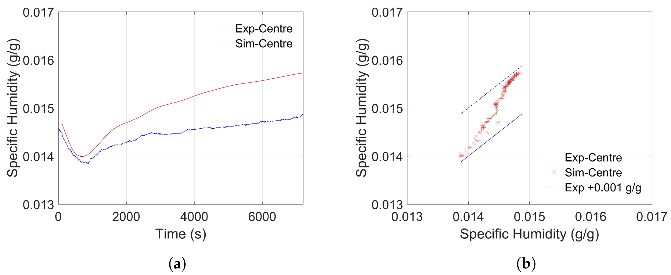
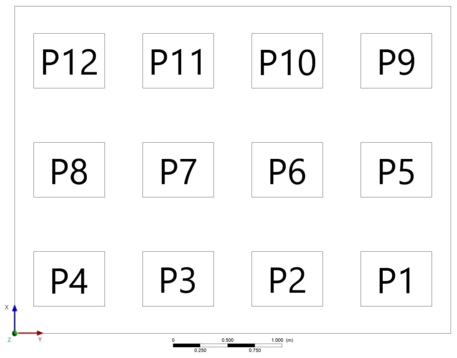
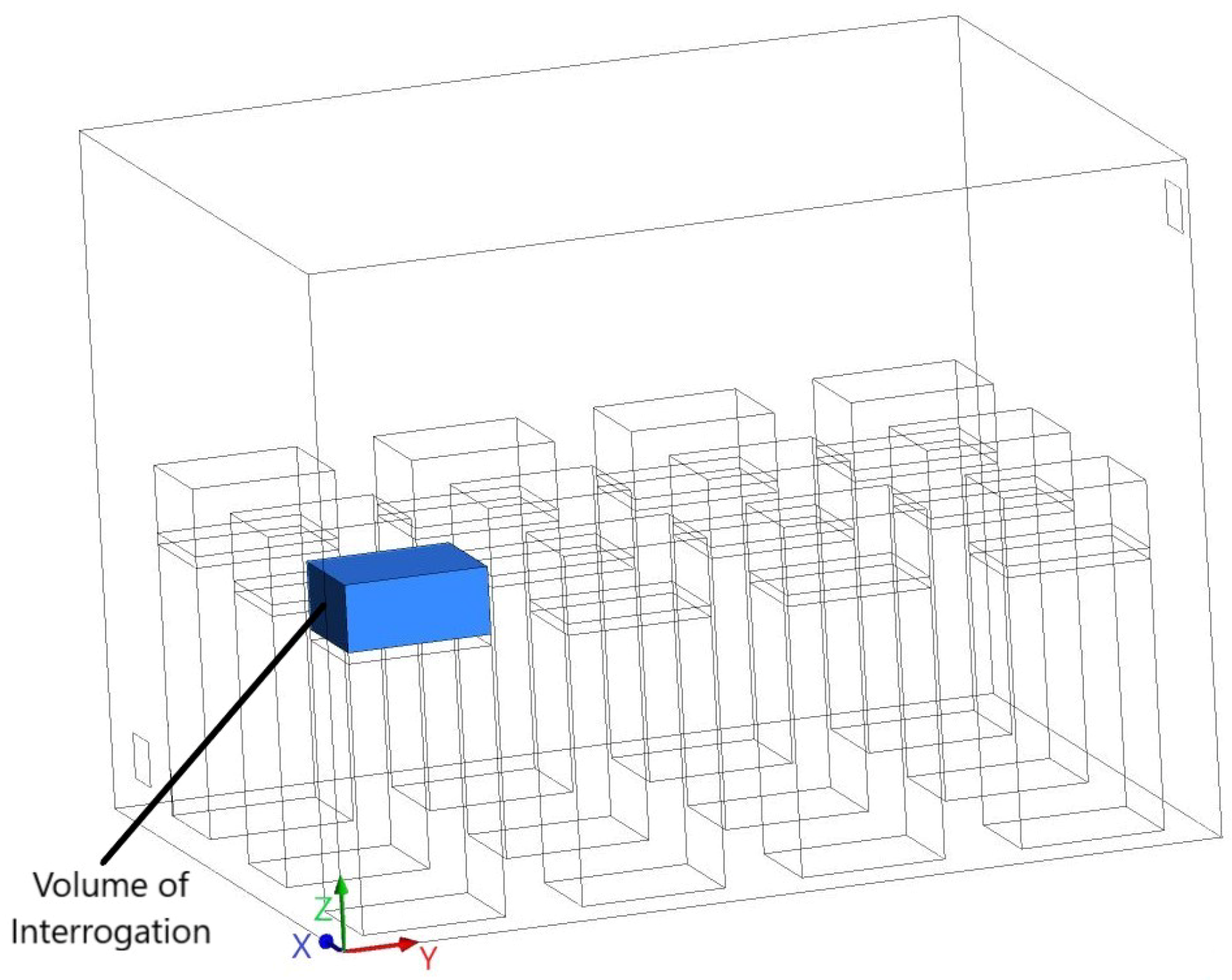
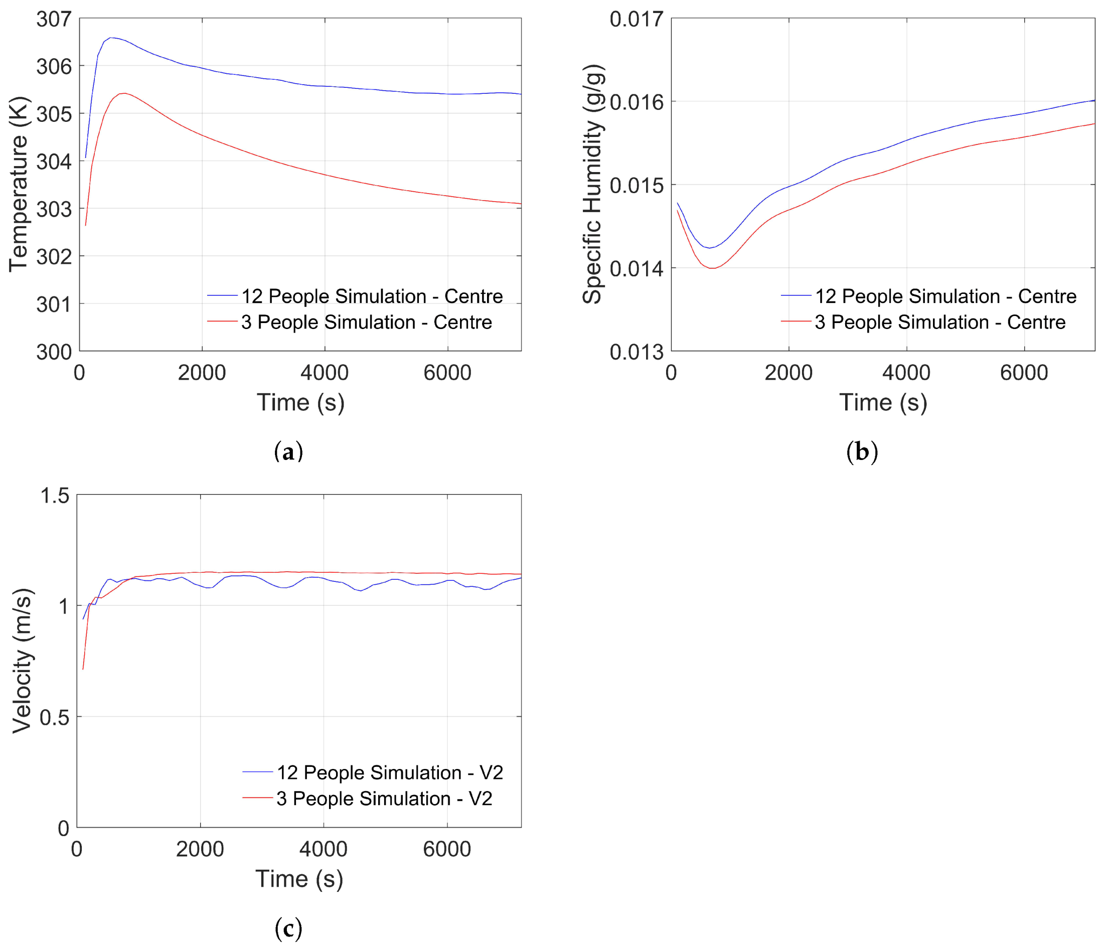
3.1. Simulation Results

To further study the effect of humidity in an internal environment, a high-density population inside the test chamber was analyzed and compared to the three person experimental test case. The three person case presented an occupancy of 4.0 ${\mathrm{m}}^2$ per person, which is typical for an office. On the other hand, an example of a high-density population is given by ASHRAE [51] as 0.7 to 0.9 ${\mathrm{m}}^2$ per person in the seated area of an opera theater. Such a definition is typically considered as having a person occupy less than 1.5 ${\mathrm{m}}^2$. Such spaces also include classrooms and cinema theaters. A high occupation density in an interior space may result in several negative health-related effects as determined by Egorov et al. [52]. To analyze the effect of humidity in a densely populated interior environment, twelve people were modeled in a four-by-three grid scenario in the 12 ${\mathrm{m}}^2$ test chamber described above, thus considering an occupation density of 1 ${\mathrm{m}}^2$ per person. The configuration adopted is shown in Figure 6.

The twelve modeled sedentary people were given the same cell and boundary conditions as the three simulated people in the validation model. This means that a skin temperature of 307.65 $\mathrm{K}$ and a humidity source of 2.5265 × 10⁻⁴ $\mathrm{k}\mathrm{g} {\mathrm{m}}^{-3} \mathrm{s}{}^{-1}$ in the 5 cm volume above each person’s head were applied. The geometry was also modified to include a volume of height 30 cm, above each person’s head, as shown in Figure 7 and as defined in Equation (6). This was taken as the volume directly above the person, in which the total mass of water vapor in the two-hour experiment may be measured. The results of the high-density occupation case (with twelve people) are compared to the three people case in Figure 8.

From Figure 8c, it is clear that the average velocity at the jet location (0.31, 2.80, 2.60 m) of the two simulations was 1.15 $\mathrm{m} \mathrm{s}{}^{-1}$. The twelve people simulation was less uniform than the three people one. Such unsteady phenomena were attributed to vortex shedding phenomena in the room due to the higher volume being occupied by the cubes representing the people. The temperature difference between the two curves in Figure 8a is the result of the presence of an extra nine people, each emitting heat at a uniform temperature of 307.65 $\mathrm{K}$, inside the test chamber. This variation in the two results at the ‘center’ location with co-ordinates (1.52, 2.20, 2.44 m) amounts to 2.3 $\mathrm{K}$ at the end of the two-hour simulation period. Figure 8b then shows that, similar to the temperature curves, the humidity curve that represented the twelve people simulation was 0.00027 $\mathrm{g} \mathrm{g}{}^{-1}$ higher than the curve that represented the three people simulation. This difference corresponds to the humidity sources from the heads of the extra nine people present in the twelve people simulation and is approximately equal to 1% relative humidity at 305.5 $\mathrm{K}$. One should note that whereas the difference in specific humidity was more or less constant ($\pm 5 \times {10}^{-6} \mathrm{g} \mathrm{g}{}^{-1}$) throughout the simulation, the temperature change increased with time.

Following the comparison between the three and twelve people models, the spatio-temporal distribution of humidity under the larger humidity source coming from the twelve sedentary people was analyzed. In order to study the localized distribution of humidity above the head of each occupant, a volume integral was calculated using Equation (6). The shape of interrogation volume was a cuboid of dimensions (0.65, 0.5, 0.3 m) as highlighted in Figure 7. The choice of height of this interrogation volume was set arbitrarily to encompass the volume above each person but to also exclude the slipstream of the jet.

$$M_h(x,y,z,t)=\int \int \int H(x,y,z,t)\times {\rho }_{a}dxdydz$$

(6)

where

• $M_h$ is the mass of water above each occupant;
• H is the total water vapor mass fraction on top of the person, calculated using the CFD program;
• ${\rho }_a$ is the average density of air on top of each person, calculated using the CFD program.

The mass flux of water vapor through the surface S of the hypothetical cuboid is given by Equation (7). The formula shows an intrinsic relation between the velocities and the mass transfer.

$$-\underset{S}{\overset{}{\int }}{\rho }_a\overrightarrow{u}·\overrightarrow{n}dS=\frac{d{M}_h}{dt}$$

(7)

where

• S is the surface of the interrogation volume;
• $\overrightarrow{u}$ is the velocity vector;
• $\overrightarrow{n}$ is the normal to the surface of the cuboid.

Given that the simulation is a transient one, and that the $M_h$ value calculated by Equation (6) is variable with time, the array of results achieved using the latter equation were then integrated over the two-hour time period using the integral $M=\int M_{h}dt$ to obtain the total amount of water vapor above the person in the whole experimental period.

The above simulation, together with the subsequent calculations, were then performed once again, with the major change of eliminating the humidity source of the twelve people. This was done to determine the amount of existing humidity already present on top of each person. This new humidity value generated by this simulation is thus not to be attributed to that person’s humidity release, but solely to the conditions of the micro-climate around them.

The difference in the humidities generated by these two simulations is thus equivalent to the mass of humidity above each person due to that person’s humidity release only, thus eliminating any humidity effects present in the test chamber micro-climate. The results are tabulated in

Table 4. Total humidity on each person in the test chamber.

Person	Mass of Water Vapour (in Grams)
	Person and Micro-Climate	Micro-Climate Without Person	Person Only
P1	12.2155	11.8279	0.3877
P2	12.2337	11.8257	0.4080
P3	12.2320	11.8257	0.4063
P4	12.1823	11.8418	0.3406
P5	12.1715	11.8390	0.3324
P6	12.1872	11.8367	0.3505
P7	12.2015	11.8340	0.3675
P8	12.1629	11.8516	0.3114
P9	12.1583	11.8538	0.3045
P10	12.1528	11.8539	0.2989
P11	12.1556	11.8516	0.3040
P12	12.1383	11.8582	0.2800

and shown in bar charts in Figure 9.

Complementing the bar charts in Figure 9, the contours in Figure 10a,b show instantaneous specific humidity values above the heads of the different people inside the test chamber. Figure 10a shows the plot at 1000 s, when the jet was at its peak dehumidification, while Figure 10b shows the plot at 7200 s, at the end of the experiment. The main difference between Figure 9 and Figure 10 is that while the latter show instantaneous plots for the specific humidity on a two-dimensional plane, the bar chart shows the total mass of water inside a volume during a two-hour period.

3.2. Discussion

Although showing different quantities, in a different configuration and different time periods, Figure 9 and Figure 10 still display similarities in their results. Figure 9b shows that the people with the greatest mass of water vapor on top of their heads during the two hours of the experiment were P1, P2, and P3, closely followed by P6 and P7. The chart shows that P12 had the least amount of water on their head. The instantaneous plots in Figure 10a,b also show that P1, P2, and P3 had the most humidity at both 1000 s and 7200 s. P6 and P7 also had a considerable amount of water vapor in the two selected moments, with P12 having the least amount of humidity in the two contours.

In accordance to the values in Table 4, the people with the highest and lowest amount of humidity (negating the effect of the micro-climate) were P2 and P12, respectively, with 0.4080 g and 0.2800 g of water above their heads during the two-hour simulation period. Even though the quantities, in themselves, are judged to be very small due to the lack of occupant activity and thus the small release of humidity by the sedentary people, the percentage difference in the mass of water above P2 and P12 was determined to be 31%, which is very significant and thus demands further analysis about the distribution of humidity in the micro-climate and the reasons behind such a contrast between the two people situated in the different locations.

The velocities above the seated models’ heads were then analyzed for the two points in time discussed above and are presented in Figure 10c,d. These contours show that, for the two instants in question, velocity was at its lowest above P1, P2, and P3, followed by P5 and P6. The highest velocity was shown to be above P12. These results correlate well with the observations on the humidity distributions. It was thus observed that the way the flow behaves directly influences the distribution of humidity in the test chamber. This corresponds with Equation (7), which states that the rate of change of water vapour mass is proportional to the velocities coming out of the surfaces of the defined interrogation volume. This study shows that, contrary to the general consensus, there are cases where the humidity distribution inside the room is not uniform. Such a case would be the one studied during this research, namely an interior space containing a considerable humidity load. Further studies should assess how the thermal comfort of the individual people inside such a micro-climate would differ due to the humidity content above their head.

Existing studies on the spatio-temporal distribution of humidity are very limited. Most studies concentrate on the humidity effect on the room walls [18] so that building material and any furniture or artefacts may be preserved. This study has, in contrast, modeled and described the whole interior micro-climate to enable a better understanding of the spatio-temporal distribution of humidity inside a room. A similar study was carried out by Huang et al. [20]. The micro-climate studied in the latter was composed of a much coarser mesh (about 73,000 cells vs. 1.8 million cells) and was designed as an intermediate model between large time step zonal models and short time step CFD analysis. These differences may well be explained by the aims of the respective research. While the analysis by Huang et al. concentrated on the verification of a new predicting factor for indoor humidity, this study aimed to show the exact distribution and change in humidity inside the room, with respect to space and time. The main similarity between the results of the two studies is they both show the humidity spatio-temporal distribution is directly related to the air flow, as described in Equation (7) and above.

4. Conclusions

This paper has described the methodology that was used to carry out humidity-related experiments in a test chamber and the subsequent modeling using a validated predictive CFD tool. The latter model was used to simulate a high-occupancy case, acting as a considerable source of humidity inside a test chamber. The conclusions of this study are as follows:

• Contrary to the general consensus that humidity distribution inside an interior living space is practically uniform, this study has shown that there may be cases where the spatio-temporal distribution of humidity varies considerably inside a room, specifically as shown in this case of high humidity.
• The case of a high-humidity source inside a test chamber was analyzed through the simulation of a high-density population inside the room. The authors determined that different locations were effected by different amounts of humidity over a two-hour period. A 31% difference was calculated between the locations having the highest and lowest masses of water in their surroundings.
• It was also determined that, as expected, the distribution of humidity was closely related to the path of air flow inside the room.
• For this specific case, it was determined that the people seated furthest from the inlet and closest to the outlet would have the least amount of water vapor above them.

This study aims to aid future designers and engineers to design and implement HVAC systems more effectively, keeping in mind the thermal comfort of building occupants, the conservation of historic buildings, and the artefacts within. Future work should concentrate on analyzing whether the differences in the mass of water vapor in a person’s proximity contribute to distinctive thermal comfort votes by each person. Additionally, other work could also examine the spatio-temporal distribution of humidity in a room with no inlet jet so as to analyze and compare the humidity distribution under purely convective and diffusive circumstances.

References

1. Kaynakli, O.; Kilic, M. Investigation of indoor thermal comfort under transient conditions. Build. Environ. 2005, 40, 165–174. [Google Scholar] [CrossRef]
2. Fanger, P.O. Thermal comfort: Analysis and applications in environmental engineering: Fanger, P.O. Danish Technical Press, Copenhagen, Denmark, 1970, 244 pp.: Abstr. in World Textile Abstracts. Appl. Ergon. 1972, 3, 181. [Google Scholar] [CrossRef]
3. Chiang, W.H.; Wang, C.Y.; Huang, J.S. Evaluation of cooling ceiling and mechanical ventilation systems on thermal comfort using CFD study in an office for subtropical region. Build. Environ. 2012, 48, 113–127. [Google Scholar] [CrossRef]
4. Ciuha, U.; Mekjavic, I.B. Regional thermal comfort zone in males and females. Physiol. Behav. 2016, 161, 123–129. [Google Scholar] [CrossRef]
5. Liu, W.; Huangfu, H.; Xiong, J.; Deng, Q. Feedback effect of human physical and psychological adaption on time period of thermal adaption in naturally ventilated building. Build. Environ. 2014, 76, 1–9. [Google Scholar] [CrossRef]
6. Requena-Ruiz, I. Thermal comfort in twentieth-century architectural heritage: Two houses of Le Corbusier and André Wogenscky. Front. Archit. Res. 2016, 5, 157–170. [Google Scholar] [CrossRef]
7. Li, B.; Du, C.; Tan, M.; Liu, H.; Essah, E.; Yao, R. Studies of the impact of air humidity on human acceptable air temperatures in hot-humid environments. Energy Build. 2017, 158, 393–405. [Google Scholar] [CrossRef]
8. Yu, B.H.; Seo, B.M.; Hong, S.H.; Yeon, S.; Lee, K.H. Influences of different operational configurations on combined effects of room air stratification and thermal decay in UFAD system. Energy Build. 2018, 176, 262–274. [Google Scholar] [CrossRef]
9. Wiriyasart, S.; Naphon, P. Numerical study on air ventilation in the workshop room with multiple heat sources. Case Stud. Therm. Eng. 2019, 13, 100405. [Google Scholar] [CrossRef]
10. Srivajana, W. Effects of Air Velocitv on Thermal Comfort in Hot and Humid Climates. Thammasat Int. J. Sci. Tech. 2003, 8, 45–54. [Google Scholar]
11. Parsons, K. Human Thermal Environments the Effects of Hot, Moderate, and Cold Environments on Human Health, Comfort, and Performance, 3rd ed.; CRC Press: Boca Raton, FL, USA, 2014. [Google Scholar]
12. Tanabe, S.; Kimura, K. Effects of air temperature, humidity, and air movement on thermal comfort under hot and humid conditions. ASHRAE Trans. 1994, 100, 953–969. [Google Scholar]
13. Zhang, H.; Yoshino, H. Analysis of indoor humidity environment in Chinese residential buildings. Build. Environ. 2010, 45, 2132–2140. [Google Scholar] [CrossRef]
14. Jin, L.; Zhang, Y.; Zhang, Z. Human responses to high humidity in elevated temperatures for people in hot-humid climates. Build. Environ. 2017, 114, 257–266. [Google Scholar] [CrossRef]
15. Tsutsumi, H.; Tanabe, S.-i.; Harigaya, J.; Iguchi, Y.; Nakamura, G. Effect of humidity on human comfort and productivity after step changes from warm and humid environment. Build. Environ. 2007, 42, 4034–4042. [Google Scholar] [CrossRef]
16. Djamila, H.; Chu, C.M.; Kumaresan, S. Effect of Humidity on Thermal Comfort in the Humid Tropics. J. Build. Constr. Plan. Res. 2014, 2, 109. [Google Scholar] [CrossRef] [Green Version]
17. Saber, E.; Mast, M.; Tham, K.W.; Leibundgut, H. Numerical Modelling of an Indoor Space Conditioned with Low Exergy Cooling Technologies in the Tropics. In Proceedings of the 13th International Conference on Indoor Air Quality and Climate, Hong Kong, China, 7–12 July 2014. [Google Scholar] [CrossRef]
18. Mortensen, L.H.; Woloszyn, M.; Rode, C.; Peuhkuri, R. Investigation of Microclimate by CFD Modeling of Moisture Interactions between Air and Constructions. J. Build. Phys. 2007, 30, 279–315. [Google Scholar] [CrossRef]
19. Wurtz, E.; Haghighat, F.; Mora, L.; Cordeiro Mendonça, K.; Maalouf, C.; ZHAO, H.; Bourdoukan, P. An integrated zonal model to predict transient indoor humidity distribution. ASHRAE Trans. 2006, 112, 175–186. [Google Scholar]
20. Huang, H.; Kato, S.; Hu, R.; Ishida, Y. Development of new indices to assess the contribution of moisture sources to indoor humidity and application to optimization design: Proposal of CRI(H) and a transient simulation for the prediction of indoor humidity. Build. Environ. 2011, 46, 1817–1826. [Google Scholar] [CrossRef]
21. Butera, F.M. Chapter 3—Principles of thermal comfort. Renew. Sustain. Energy Rev. 1998, 2, 39–66. [Google Scholar] [CrossRef]
22. Lefevre, J. Chaleur Animale et Energetigue; Masson: Paris, France, 1911. [Google Scholar]
23. Burton, A.C. The Application of the Theory of Heat Flow to the Study of Energy Metabolism: Five Figures. J. Nutr. 1934, 7, 497–533. [Google Scholar] [CrossRef]
24. Tanabe, S.; Kobayashi, K.; Nakano, J.; Ozeki, Y.; Konishi, M. Evaluation of thermal comfort using combined multi-node thermoregulation (65MN) and radiation models and computational fluid dynamics (CFD). Energy Build. 2002, 34, 637–646. [Google Scholar] [CrossRef] [Green Version]
25. Fiala, D.; Lomas, K.J.; Stohrer, M. A computer model of human thermoregulation for a wide range of environmental conditions: The passive system. J. Appl. Physiol. 1999, 87, 1957–1972. [Google Scholar] [CrossRef]
26. Kingma, B.R.M.; Schellen, L.; Frijns, A.J.H.; van Marken Lichtenbelt, W.D. Thermal sensation: A mathematical model based on neurophysiology. Indoor Air 2012, 22, 253–262. [Google Scholar] [CrossRef] [Green Version]
27. Dubois, D.; Dubois, E.F. A formula to estimate the approximate area if height and weight be known. Arch. Intern. Med. (Chic) 1916, 17, 863–871. [Google Scholar] [CrossRef] [Green Version]
28. Katić, K.; Li, R.; Zeiler, W. Thermophysiological models and their applications: A review. Build. Environ. 2016, 106, 286–300. [Google Scholar] [CrossRef] [Green Version]
29. Gagge, A.P. An Effective Temperature Scale Based on a Simple Model of Human Physiological Regulatory Response. ASHRAE Trans. 1971, 77, 247–262. [Google Scholar]
30. Stolwijk, J. A Mathematical Model of Physiological Temperature Regulation in Man; Number v. 1855 in NASA Contractor Report; National Aeronautics and Space Administration: Washington, DC, USA, 1971.
31. Fiala, D.; Havenith, G.; Bröde, P.; Kampmann, B.; Jendritzky, G. UTCI-Fiala multi-node model of human heat transfer and temperature regulation. Int. J. Biometeorol. 2012, 56, 429–441. [Google Scholar] [CrossRef] [Green Version]
32. Cook, M.; Cropper, P.; Fiala, D.; Yousaf, R.; Bolineni, S.; van Treeck, C. Coupled CFD and Thermal Comfort Modeling in Cross-Ventilated Classrooms. ASHRAE Trans. 2013, 119, 1–8. [Google Scholar]
33. Dixit, A.; Gade, U. A case study on human bio-heat transfer and thermal comfort within CFD. Build. Environ. 2015, 94, 122–130. [Google Scholar] [CrossRef]
34. Onset. HOBO UX100-003 Data Logger. Original Datasheet from Onset. Available online: www.onsetcomp.com/datasheet/UX100-003 (accessed on 15 March 2017).
35. Lascar-Electronics. EL-WiFi-21CFR-TH. Original Datasheet from Lascar Electronics. Available online: https://docs-emea.rs-online.com/webdocs/15e9/0900766b815e9e66.pdf (accessed on 22 August 2016).
36. Kimo-Instruments. MP 210. Original Datasheet from Kimo Instruments. Available online: http://kimo-instruments.com/sites/kimo/{\@@par}les/2017-09/FTang_portable_MP210-25-08-170.pdf (accessed on 25 August 2017).
37. Kimo-Instruments. SFC900GN. Original Datasheet from Kimo Instruments. Available online: www.kimo.it/wp-content/uploads/2016/10/24782.pdf (accessed on 24 October 2016).
38. ISO 9972. Thermal Performance of Buildings—Determination of Air Permeability of Buildings—Fan Pressurization Method; Standard; International Organization for Standardization: Geneva, Switzerland, 2015. [Google Scholar]
39. ASTM E779-19. Standard Test Method for Determining Air Leakage Rate by Fan Pressurization; Standard; ASTM International: West Conshohocken, PA, USA, 2019. [Google Scholar] [CrossRef]
40. ASTM E741-11. Standard Test Method for Determining Air Change in a Single Zone by Means of a Tracer Gas Dilution; Standard; ASTM International: West Conshohocken, PA, USA, 2017. [Google Scholar] [CrossRef]
41. Sherman, M.H. Comparison of Methods for the Measurement of Air Change Rates and Interzonal Airflows in Two Test Residences. In Air Change Rate and Airtightness in Buildings: Symposium: Papers; ASTM: Philadelphia, PA, USA, 1990; pp. 104–113. [Google Scholar]
42. Roulet, C.A.; Foradini, F. Simple and Cheap Air Change Rate Measurement Using CO2 Concentration Decays. Int. J. Vent. 2002, 1, 39–44. [Google Scholar] [CrossRef]
43. ASHRAE. Chapter 16—Ventilation and Infiltration. In 2017 ASHRAE Handbook—Fundamentals (SI Edition); ASHRAE: Atlanta, GA, USA, 2017. [Google Scholar]
44. Bonello, M.; Micallef, D.; Borg, S. Flat Bed Desiccant Dehumidification: A predictive model for desiccant transient characterisation using a species transport model within CFD. J. Build. Eng. 2019, 23, 280–290. [Google Scholar] [CrossRef]
45. ANSYS. 1994. Available online: ansys56manual.pdf (accessed on 24 December 2020).
46. University of Malta. Overview_of_Albert; University of Malta: Msida, Malta, 2012. [Google Scholar]
47. Yang, Z.; Shih, T. New time scale based k-epsilon model for near-wall turbulence. AIAA J. 1993, 31, 1191–1198. [Google Scholar] [CrossRef] [Green Version]
48. Bonello, M.; Micallef, D.; Borg, S. Humidity micro-climate characterisation in indoor environments: A benchmark study. J. Build. Eng. 2020, 28, 101013. [Google Scholar] [CrossRef]
49. Roache, P.J. Verification and Validation in Computational Science and Engineering; Hermosa Publishers: Socorro, NM, USA, 1998; pp. 107–141. [Google Scholar]
50. Zielinski, J.; Przybylski, J. How much water is lost during breathing? Pneumonol. Alergol. Pol. 2012, 80, 339–342. [Google Scholar]
51. ASHRAE. Chapter 5—Places of Assembly. In 2015 ASHRAE Handbook: Heating, Ventilating, and Air-Conditioning Applications, SI ed.; ASHRAE: Atlanta, GA, USA, 2015. [Google Scholar]
52. Egorov, A.; Martuzzi, M.; Krzyzanowski, M.; Hänninen, O.; Haverinen-Shaughnessy, U.; Täubel, M.; Geiss, O.; Kephalopoulos, S.; Barrero, J.; Wendland, C.; et al. School Environment: Policies and Current Status; World Health Organization: Geneva, Switzerland, 2015. [Google Scholar]
Figure 1. Sketch of the experimental test chamber.
Energies 14 00681 g001
Figure 2. Time-varying conditions at the inlet. (a) Inlet temperature; (b) inlet specific humidity.
Energies 14 00681 g002
Figure 3. Mesh for the test chamber CFD model.
Energies 14 00681 g003
Figure 4. Time-step independence verification. (a) Temperature variable; (b) specific humidity variable.
Energies 14 00681 g004
Figure 5. Validation of CFD model results at point ‘center’. (a) Specific humidity—results; (b) specific humidity—comparison.
Energies 14 00681 g005
Figure 6. Z-Plane showing room geometry and grid of 12 seated people.
Energies 14 00681 g006
Figure 7. Sketch of the 12 people simulation model.
Energies 14 00681 g007
Figure 8. Results of simulations with 3 and 12 modeled, seated people inside the test chamber. (a) Temperature at the center; (b) specific humidity at the centre; (c) velocity at the jet.
Energies 14 00681 g008
Figure 9. Total mass of water on top of each person’s head. (a) Mass of water—person and micro-climate (blue); micro-climate without person (yellow); (b) mass of water—person only.
Energies 14 00681 g009
Figure 10. Instantaneous specific humidity and velocity plots for different times during simulation. (a) Specific humidity at 1000 s; (b) specific humidity at 7200 s; (c) velocity at 1000 s; (d) velocity at 7200 s.
Energies 14 00681 g010