
Dry and Wet Climate Periods over Eastern South America: Identification and Characterization through the SPEI Index

 ,
,  ,
,  ,
, 
 ,
,  ,
, 
Abstract
1. Introduction
2. Data and Methodology
2.1. Data
2.2. Definition of the Lagrangian Approach for the Moisture Transport Analysis and the Study Area
2.3. Identification and Characterization of Wet and Dry Climate Periods through SPEI
- The classification of monthly SPEI values according to their magnitude (Table 1);
- The identification of the domain-scale dry and wet events. A wet (dry) event starts when the SPEI value first falls above (below) zero (month included), followed by a value of 1 or higher (–1 or less), and ends when the SPEI returns to a negative (positive) value (month not included).
- Severity represents the absolute sum of all SPEI values during the event;
- Duration signifies the number of months between the first and last month of the event;
- Intensity is calculated as the ratio between the severity and duration;
- Peak value is the highest absolute SPEI value registered during the event.
3. Results
4. Summary and Conclusions
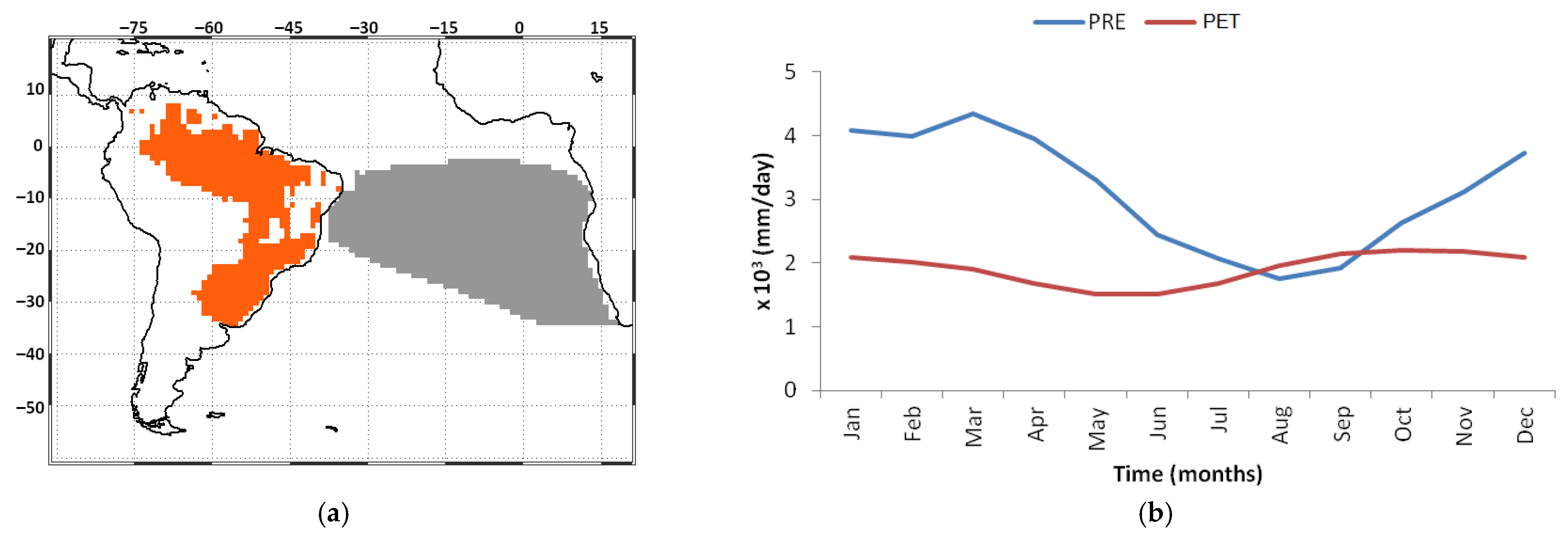
- The climatological annual cycle of the freshwater flux over ESA shows that precipitation prevailed over potential evapotranspiration during the year, except from August to September. ESA is characterized by rainier Summer months and a drier Winter season.
- Although the decade of 1980 presented the highest number of extremely wet values in the SPEI-1, -3, -6, and -12 accumulation periods, it was also characterized by the predominance of dry values in the SPEI-3, -6, and -12 scales. The most intense dry events (also presenting the highest peaks) at SPEI-3 and SPEI-6 were identified during the 1980s. However, most of the wet events presenting the highest magnitude of the parameters investigated at the four scales have been registered during the decade of 1980. In other words, results indicate that wet and dry conditions occurred during this period.
- Both approaches confirm the predominance of wet conditions during the decade of 1990 and 2000, except for the SPEI-1. It is worth noting that the decade of 1990 presented the highest number of extremely dry values in the SPEI-1time series, registering the dry event with the highest peak at SPEI-1.
- The 2010s concentrates the highest number of occurrences of dry SPEI values, particularly the moderate ones. The longest and more severe dry events at the four scales have been identified during this period.
Supplementary Materials
Author Contributions
Funding
Acknowledgments
Conflicts of Interest
References
- Intergovernmental Panel on Climate Change (IPCC). Climate Change 2014: Synthesis Report; Contribution of Working Groups I, II and III to the Fifth Assessment Report of the Intergovernmental Panel on Climate Change; Pachauri, R.K., Meyer, L.A., Eds.; IPCC: Geneva, Switzerland, 2014; 151p, Available online: https://www.ipcc.ch/pdf/assessment-report/ar5/syr/SYR_AR5_FINAL_full_wcover.pdf (accessed on 23 January 2021).
- Marengo, J.A.; Nobre, C.A.; Tomasella, J.; Cardoso, M.F.; Oyama, M.D. Hydro-climatic and ecological behaviour of the drought of Amazonia in 2005. Philos. Trans. R. Soc. B 2008, 363, 1773–1778. [Google Scholar] [CrossRef] [PubMed]
- Marengo, J.A.; Alves, L.M.; Soares, W.R.; Rodriguez, D.A.; Camargo, H.; Riveros, M.P.; Pabló, A.D. Two Contrasting Severe Seasonal Extremes in Tropical South America in 2012: Flood in Amazonia and Drought in Northeast Brazil. J. Clim. 2013, 26, 9137–9154. [Google Scholar] [CrossRef]
- Garreaud, R.D.; Alvarez-Garreton, C.; Barichivich, J.; Boisier, J.P.; Christie, D.; Galleguillos, M.; LeQuesne, C.; McPhee, J.; Zambrano-Bigiarini, M. The 2010–2015 megadrought in Central Chile: Impacts on regional hydroclimate and vegetation. Hydrol. Earth Syst. Sci. 2017, 21, 6307–6327. [Google Scholar] [CrossRef]
- Drumond, A.; Stojanovic, M.; Nieto, R.; Vicente-Serrano, S.M.; Gimeno, L. Linking anomalous moisture transport and drought episodes in the IPCC reference regions. Bull. Am. Meteorol. Soc. 2019, 100, 1481–1498. [Google Scholar] [CrossRef]
- Coelho, C.A.S.; de Oliveira, C.P.; Ambrizzi, T.; Reboita, M.S.; Bertoletti Carpenedo, C.; Pereira Silveira Campos, J.L.; Nóbile Tomaziello, A.C.; Nóbile Tomaziello, L.; de Souza Custódio, M.; Mosso Dutra, L.M.; et al. The 2014 southeast Brazil austral summer drought: Regional scale mechanisms and teleconnections. Clim. Dyn. 2016, 46, 3737–3752. [Google Scholar] [CrossRef]
- Otto, F.E.L.; Haustein, K.; Uhe, P.; Coelho, C.A.S.; Aravequia, J.K.; Almeida, W.; King, A.; Coughlan de Perez, E.; Wada, Y.; van Oldenborgh, G.J.; et al. Factors other than climate change, main drivers of 2014/15 water shortage in southeast Brazil. Bull. Am. Meteorol. Soc. 2015, 96, S1–S172. [Google Scholar] [CrossRef]
- Nobre, C.A.; Marengo, J.A.; Seluchi, M.E.; Cuartas, A.; Alves, L.M. Some Characteristics and Impacts of the Drought and Water Crisis in Southeastern Brazil during 2014 and 2015. J. Water Resour. Prot. 2016, 8, 252–262. [Google Scholar] [CrossRef]
- Marengo, J.A.; Espinoza, J.C. Extreme seasonal droughts and floods in Amazonia: Causes, trends and impacts. Int. J. Climatol. 2016, 36, 1033–1050. [Google Scholar] [CrossRef]
- Marengo, J.A., Jr.; Souza, C.; Thonicke, K.; Burton, C.; Halladay, K.; Betts, R.A.; Alves, L.M.; Soares, W.R. Changes in Climate and Land Use Over the Amazon Region: Current and Future Variability and Trends. Front. Earth Sci. 2018, 6, 228. [Google Scholar] [CrossRef]
- Espinoza, J.C.; Marengo, J.A.; Ronchai, J.; Molina Carpio, J.; Noriega Flores, L.; Loup Guyot, J. The extreme 2014 flood in south-western Amazon basin: The role of tropical-subtropical South Atlantic SST gradient. Environ. Res. Lett. 2014, 9, 124007. [Google Scholar] [CrossRef]
- Marengo, J.A.; Torres, R.R.; Alves, L.M. Drought in Northeast Brazil—Past, present, and future. Theor. Appl. Climatol. 2017, 129, 1189–1200. [Google Scholar] [CrossRef]
- Marengo, J.A.; Alves, L.M.; Alvalá, R.C.; Cunha, A.P.; Brito, S.; Moraes, O.L. Climatic characteristics of the 2010–2016 drought in the semiarid Northeast Brazil region. An. Acad. Bras. Cienc. 2017, 90, 1973–1985. [Google Scholar] [CrossRef]
- Brazil Fires Burn World´s Largest Tropical Wetlands at ´Unprecedented´ Scale. Available online: https://www.nytimes.com/2020/09/04/world/americas/brazil-wetlands-fires-pantanal.html (accessed on 18 January 2021).
- Palmer, W.C. Meteorological Drought; White, R.M., Ed.; U.S. Weather Bureau: Washington, DC, USA, 1965. Available online: https://www.ncdc.noaa.gov/temp-and-precip/drought/docs/palmer.pdf (accessed on 17 December 2020).
- McKee, T.B.; Doesken, N.J.; Kleist, J. The relationship of drought frequency and duration to time scales. In Proceedings of the Eighth Conference on Applied Climatology, Boston, MA, USA, 17–22 January 1993; pp. 179–184. Available online: https://www.droughtmanagement.info/literature/AMS_Relationship_Drought_Frequency_Duration_Time_Scales_1993.pdf (accessed on 17 December 2020).
- Hayes, M.; Svodoba, M.; Wall, N.; Widhalm, M. The Lincoln Declaration on Drought Indices: Universal meteorological drought index recommended. Bull. Am. Meteorol. Soc. 2011, 92, 485–488. [Google Scholar] [CrossRef]
- Otkin, J.A.; Svoboda, M.; Hunt, E.D.; Ford, T.W.; Anderson, M.C.; Hain, C.; Basara, B. Flash droughts: A review and assessment of the challenges imposed by rapid-onset droughts in the United States. Bull. Am. Meteorol. Soc. 2017, 99, 911–919. [Google Scholar] [CrossRef]
- Vicente-Serrano, S.M.; Begueria, S.; Lopez-Moreno, J.I. A multiscalar drought index sensitive to global warming: The Standardized Precipitation Evapotranspiration Index. J. Clim. 2010, 23, 1696–1718. [Google Scholar] [CrossRef]
- Cunha, A.P.M.A.; Zeri, M.; Deusdará Leal, K.; Costa, L.; Cuartas, L.A.; Marengo, J.A.; Tomasella, J.; Vieira, R.M.; Barbosa, A.A.; Cunningham, C.; et al. Extreme Drought Events over Brazil from 2011 to 2019. Atmosphere 2019, 10, 642. [Google Scholar] [CrossRef]
- Drumond, A.; Stojanovic, M.; Nieto, R.; Gimeno, L.; Liberato, M.L.R.; Ambrizzi, T.; Pauliquevis, T.; de Oliveira, M. Analysis of Dry and Wet Episodes in Eastern South America During 1980–2018 Using SPEI. In Proceedings of the 3rd International Electronic Conference on Atmospheric Sciences, ECAS-2020, Online Conference, 16–30 November 2020. [Google Scholar] [CrossRef]
- Dee, D.P.; Uppala, S.M.; Simmons, A.J.; Berrisford, P.; Poli, P.; Kobayashi, S.; Andrae, U.; Balmaseda, M.A.; Balsamo, G.; Bauer, P.; et al. The ERA-Interim reanalysis: Configuration and performance of the data assimilation system. Q. J. R. Meteorol. Soc. 2001, 137, 553–597. [Google Scholar] [CrossRef]
- Stohl, A.; Forster, C.; Frank, A.; Seibert, P.; Wotawa, G. Technical note: The Lagrangian particle dispersion model FLEXPART version 6.2. Atmos. Chem. Phys. 2005, 5, 2461–2474. [Google Scholar] [CrossRef]
- Gimeno, L.; Nieto, R.; Drumond, A.; Castillo, R.; Trigo, R.M. Influence of the intensification of the major oceanic moisture sources on continental precipitation. Geophys. Res. Lett. 2013, 40, 1443–1450. [Google Scholar] [CrossRef]
- Berrisford, P.; Dee, D.P.; Fielding, K.; Fuentes, M.; Kallberg, P.; Kobayashi, S.; Uppala, S.M. The ERA-Interim Archive; ERA Report Series, 2009, No. 1; ECMWF: Reading, UK; Available online: https://www.ecmwf.int/node/8173 (accessed on 26 January 2021).
- Harris, I.; Osborn, T.J.; Jones, P.; Lister, D. Version 4 of the CRU TS monthly high-resolution gridded multivariate climate dataset. Sci. Data 2020, 7, 109. [Google Scholar] [CrossRef]
- University of East Anglia Climatic Research, Unit; Harris, I.C.; Jones, P.D. CRU TS4.03: Climatic Research Unit (CRU) Time-Series (TS) version 4.03 of high-resolution gridded data of month-by-month variation in climate (Jan. 1901–Dec. 2018). Centre Environ. Data Anal. 2020. [Google Scholar] [CrossRef]
- Gimeno, L.; Drumond, A.; Nieto, R.; Trigo, R.M.; Stohl, A. On the origin of continental precipitation. Geophys. Res. Lett. 2010, 37, L13804. [Google Scholar] [CrossRef]
- Reboita, M.S.; Ambrizzi, T.; Silva, B.A.; Pinheiro, R.F.; Porfírio da Rocha, R. The South Atlantic Subtropical Anticyclone: Present and Future Climate. Front. Earth Sci. 2019, 7, 1–15. [Google Scholar] [CrossRef]
- Stohl, A.; James, P. A Lagrangian Analysis of the Atmospheric Branch of the Global Water Cycle. Part I: Method Description, Validation, and Demonstration for the August 2002 Flooding in Central Europe. J. Hydrometeorol. 2004, 5, 656–678. [Google Scholar] [CrossRef]
- Stohl, A.; James, P. A Lagrangian analysis of the atmospheric branch of the global water cycle: Part II: Moisture Transports between Earth’s Ocean Basins and River Catchments. J. Hydrometeorol. 2005, 6, 961–984. [Google Scholar] [CrossRef]
- Gimeno, L.; Stohl, A.; Trigo, R.M.; Domínguez, F.; Yoshimura, K.; Yu, L.; Drumond, A.; Durán-Quesada, A.M.; Nieto, R. Oceanic and Terrestrial Sources of Continental Precipitation. Rev. Geophys. 2012, 50, RG4003. [Google Scholar] [CrossRef]
- Drumond, A.; Marengo, J.M.; Ambrizzi, T.; Nieto, R.; Moreira, L.; Gimeno, L. The role of Amazon Basin moisture on the atmospheric branch of the hydrological cycle: A Lagrangian analysis. Hydrol. Earth Syst. Sci. 2014, 18, 2577–2598. [Google Scholar] [CrossRef]
- Pampuch, L.A.; Drumond, A.; Gimeno, L.; Ambrizzi, T. Anomalous patterns of SST and moisture sources in the South Atlantic Ocean associated with dry events in southeastern Brazil. Int. J. Climatol. 2016, 36, 4913–4928. [Google Scholar] [CrossRef]
- Sorí, R.; Marengo, J.M.; Nieto, R.; Drumond, A.; Gimeno, L. The Atmospheric Branch of the Hydrological Cycle over the Negro and Madeira River Basins in the Amazon Region. Water 2018, 10, 738. [Google Scholar] [CrossRef]
- Gimeno, L.; Vázquez, M.; Eiras-Barca, J.; Sorí, R.; Stojanovic, M.; Algarra, I.; Nieto, R.; Ramos, A.M.; Durán-Quesada, A.M.; Dominguez, F. Recent progress on the sources of continental precipitation as revealed by moisture transport analysis. Earth Sci. Rev. 2020, 201, 103070. [Google Scholar] [CrossRef]
- Numaguti, A. Origin and recycling processes of precipitating water over the Eurasian continent: Experiments using an atmospheric general circulation model. J. Geophys. Res. Atmos. 1999, 104, 1957–1972. [Google Scholar] [CrossRef]
- Drumond, A.; Nieto, R.; Gimeno, L.; Trigo, R.M.; Ambrizzi, T.; De Souza, E. A Lagrangian Identification of the Main Sources of Moisture Affecting Northeastern Brazil during Its Pre-Rainy and Rainy Seasons. PLoS ONE 2010, 5, e11205. [Google Scholar] [CrossRef] [PubMed]
- Drumond, A.; Nieto, R.; Gimeno, L.; Ambrizzi, T. A Lagrangian identification of major sources of moisture over Central Brazil and La Plata Basin. J. Geophys. Res. Atmos. 2008, 113, D14128. [Google Scholar] [CrossRef]
- Nogués-Paegle, J.; Mechoso, C.R.; Fu, R.; Berbery, E.H.; Chao, W.C.; Chen, T.C.; Cook, K.; Diaz, A.F.; Enfield, D.; Ferreira, R.; et al. Progress in pan American CLIVAR research: Understanding the south American monsoon. Meteorologica 2002, 27, 1–30. Available online: https://www.jsg.utexas.edu/fu/files/Nogues_Paegle_2002.pdf (accessed on 23 January 2021).
- Stojanovic, M.; Drumond, A.; Nieto, R.; Gimeno, L. Variations in moisture supply from the Mediterranean Sea during meteorological drought episodes over central Europe. Atmosphere 2018, 9, 278. [Google Scholar] [CrossRef]
- Beguería, S.; Vicente-Serrano, S.M.; Reig, F.; Latorre, B. Standardized Precipitation Evapotranspiration Index (SPEI) revisited: Parameter fitting, evapotranspiration models, tools, datasets and drought monitoring. Int. J. Climatol. 2014, 34, 3001–3023. [Google Scholar] [CrossRef]
- Vicente-Serrano, S.M.; Beguería, S. Short communication comment on “candidate distributions for climatological drought indices (SPI and SPEI)” by James H. Stagge et al. Int. J. Climatol. 2016, 36, 2120–2131. [Google Scholar] [CrossRef]
- Marengo, J.A.; Ambrizzi, T.; Lincoln, M.A.; Barreto, N.J.C.; Reboita, M.S.; Ramos, A.M. Changing Trends in Rainfall Extremes in the Metropolitan Area of São Paulo: Causes and Impacts. Front. Clim. 2020, 2, 1–13. [Google Scholar] [CrossRef]
- Rodwell, M.J.; Hoskins, B.J. Subtropical anticyclones and summer monsoons. J. Clim. 2001, 14, 3192–3211. [Google Scholar] [CrossRef]


| SPEI | Category |
| 2.0 and more | Extremely wet |
| 1.5 to 1.99 | Severely wet |
| 1.0 to 1.49 | Moderately wet |
| 0.0 to 0.99 | Mild wet |
| −0.99 to 0.0 | Mild dry |
| −1.0 to −1.49 | Moderately dry |
| −1.5 to −1.99 | Severely dry |
| −2.0 and less | Extremely dry |
| Start Date | End Date | Duration (Months) | Severity | Intensity | Peak | Start Date | End Date | Duration (Months) | Severity | Intensity | Peak |
| SPEI-1 | SPEI-3 | ||||||||||
| 03/1980 | 05/1980 | 3 | 4.33 | 1.44 | 1.91 | 03/1980 | 10/1980 | 8 | 8.11 | 1.01 | 1.87 |
| 07/1980 | 10/1980 | 4 | 2.22 | 0.56 | 1.60 | 02/1981 | 09/1981 | 8 | 9.13 | 1.14 | 2.01 |
| 02/1981 | 05/1981 | 4 | 6.04 | 1.51 | 1.96 | 06/1983 | 08/1983 | 3 | 3.19 | 1.06 | 1.27 |
| 07/1981 | 07/1981 | 1 | 1.69 | 1.69 | 1.69 | 11/1983 | 03/1984 | 5 | 3.13 | 0.63 | 1.33 |
| 04/1982 | 05/1982 | 2 | 1.42 | 0.71 | 1.15 | 01/1987 * | 04/1987 * | 4 | 6.43 | 1.61 | 2.46 * |
| 01/1983 | 03/1983 | 3 | 1.55 | 0.52 | 1.01 | 06/1987 | 05/1988 | 12 | 11.24 | 0.94 | 1.73 |
| 06/1983 | 07/1983 | 2 | 2.72 | 1.36 | 1.87 | 08/1988 | 02/1989 | 7 | 3.59 | 0.51 | 1.18 |
| 11/1983 | 02/1984 | 4 | 2.47 | 0.62 | 1.14 | 02/1991 | 07/1991 | 6 | 5.05 | 0.84 | 1.69 |
| 11/1984 | 12/1984 | 2 | 2.06 | 1.03 | 1.15 | 10/1991 | 08/1992 | 11 | 12.99 | 1.18 | 2.04 |
| 01/1986 | 02/1986 | 2 | 1.97 | 0.98 | 1.36 | 12/1992 | 08/1993 | 9 | 7.99 | 0.89 | 1.81 |
| 12/1986 | 02/1987 | 3 | 4.92 | 1.64 | 2.16 | 12/1994 | 03/1995 | 4 | 2.53 | 0.63 | 1.03 |
| 05/1987 | 06/1987 | 2 | 2.23 | 1.11 | 1.41 | 05/1995 | 10/1995 | 6 | 4.10 | 0.68 | 1.26 |
| 08/1987 | 12/1987 | 5 | 4.33 | 0.87 | 1.88 | 06/1997 | 10/1997 | 5 | 6.36 | 1.27 | 1.54 |
| 02/1988 | 03/1988 | 2 | 2.05 | 1.03 | 1.34 | 10/1999 | 01/2000 | 4 | 2.72 | 0.68 | 1.01 |
| 08/1988 | 11/1988 | 4 | 3.16 | 0.79 | 1.52 | 02/2001 | 09/2001 | 8 | 6.45 | 0.81 | 1.43 |
| 02/1991 * | 05/1991 * | 4 | 4.65 | 1.16 | 2.28 * | 03/2003 | 06/2003 | 4 | 3.43 | 0.86 | 1.02 |
| 08/1991 | 01/1992 | 6 | 6.02 | 1.00 | 2.11 | 11/2003 | 01/2004 | 3 | 1.90 | 0.63 | 1.10 |
| 03/1992 | 07/1992 | 5 | 4.27 | 0.85 | 2.08 | 08/2004 | 02/2005 | 7 | 6.82 | 0.97 | 1.76 |
| 03/1993 | 06/1993 | 4 | 4.34 | 1.09 | 2.08 | 08/2005 | 11/2005 | 4 | 3.14 | 0.79 | 1.24 |
| 04/1994 | 05/1994 | 2 | 1.33 | 0.67 | 1.11 | 08/2006 | 10/2006 | 3 | 2.95 | 0.98 | 1.51 |
| 12/1994 | 01/1995 | 2 | 2.11 | 1.06 | 1.09 | 06/2007 | 12/2007 | 7 | 4.01 | 0.57 | 1.40 |
| 07/1995 | 10/1995 | 4 | 3.30 | 0.83 | 1.97 | 10/2010 | 12/2010 | 3 | 2.58 | 0.86 | 1.37 |
| 04/1997 | 10/1997 | 7 | 5.98 | 0.85 | 1.48 | 08/2011 | 10/2011 | 3 | 2.59 | 0.86 | 1.39 |
| 08/1999 | 08/1999 | 1 | 1.16 | 1.16 | 1.16 | 05/2012 | 05/2013 | 13 | 13.34 | 1.03 | 1.59 |
| 10/1999 | 11/1999 | 2 | 2.01 | 1.00 | 1.27 | 06/2014 | 11/2014 | 6 | 2.58 | 0.43 | 1.15 |
| 01/2001 | 05/2001 | 5 | 3.72 | 0.74 | 1.76 | 02/2015 | 04/2015 | 3 | 2.60 | 0.87 | 1.00 |
| 07/2001 | 08/2001 | 2 | 2.70 | 1.35 | 1.40 | 09/2015 | 04/2018 | 32 | 31.64 | 0.99 | 2.18 |
| 02/2002 | 02/2002 | 1 | 1.01 | 1.01 | 1.01 | SPEI-6 | |||||
| 01/2003 | 01/2003 | 1 | 1.12 | 1.12 | 1.12 | 04/1980 | 12/1980 | 9 | 8.02 | 0.89 | 1.87 |
| 03/2003 | 05/2003 | 3 | 2.19 | 0.73 | 1.06 | 03/1981 * | 10/1981 * | 8 | 11.32 | 1.41 | 2.05 * |
| 10/2003 | 12/2003 | 3 | 2.37 | 0.79 | 1.48 | 02/1987 | 08/1988 | 19 | 19.59 | 1.03 | 1.77 |
| 06/2004 | 06/2004 | 1 | 1.01 | 1.01 | 1.01 | 02/1991 | 11/1992 | 22 | 23.77 | 1.08 | 1.90 |
| 08/2004 | 09/2004 | 2 | 1.51 | 0.76 | 1.24 | 02/1993 | 09/1993 | 8 | 9.60 | 1.20 | 1.68 |
| 11/2004 | 02/2005 | 4 | 4.27 | 1.07 | 2.01 | 07/1997 | 11/1997 | 5 | 4.66 | 0.93 | 1.69 |
| 06/2005 | 08/2005 | 3 | 2.32 | 0.77 | 1.73 | 03/2001 | 10/2001 | 8 | 6.57 | 0.82 | 1.26 |
| 10/2005 | 11/2005 | 2 | 1.27 | 0.63 | 1.02 | 08/2004 | 04/2005 | 9 | 7.39 | 0.82 | 1.65 |
| 01/2006 | 02/2006 | 2 | 1.61 | 0.80 | 1.11 | 11/2005 | 02/2006 | 4 | 1.52 | 0.38 | 1.04 |
| 07/2006 | 09/2006 | 3 | 3.16 | 1.05 | 1.43 | 09/2007 | 12/2007 | 4 | 2.93 | 0.73 | 1.15 |
| 06/2007 | 07/2007 | 2 | 1.25 | 0.63 | 1.10 | 05/2012 | 05/2013 | 13 | 16.10 | 1.24 | 2.01 |
| 09/2007 | 11/2007 | 3 | 2.99 | 1.00 | 1.76 | 09/2015 | 08/2018 | 36 | 41.19 | 1.14 | 2.01 |
| 04/2009 | 05/2009 | 2 | 2.02 | 1.01 | 1.43 | SPEI-12 | |||||
| 08/2010 | 11/2010 | 4 | 3.47 | 0.87 | 1.28 | 09/1980 | 03/1982 | 19 | 18.51 | 0.97 | 1.44 |
| 06/2011 | 09/2011 | 4 | 3.65 | 0.91 | 1.40 | 01/1983 | 05/1984 | 17 | 10.99 | 0.65 | 1.03 |
| 12/2011 | 12/2011 | 1 | 1.80 | 1.80 | 1.80 | 06/1987 | 07/1989 | 26 | 24.88 | 0.96 | 1.86 |
| 03/2012 | 01/2013 | 11 | 9.04 | 0.82 | 1.63 | 03/1991 | 01/1994 | 35 | 37.76 | 1.08 | 1.96 |
| 03/2013 | 04/2013 | 2 | 1.42 | 0.71 | 1.21 | 06/2004 | 05/2005 | 12 | 5.77 | 0.48 | 1.29 |
| 12/2013 | 01/2014 | 2 | 2.36 | 1.18 | 1.20 | 05/2012 | 10/2013 | 18 | 18.81 | 1.04 | 1.79 |
| 05/2014 | 10/2014 | 6 | 3.06 | 0.51 | 1.36 | 02/2015 * | 10/2018 * | 45 | 55.52 | 1.23 | 2.10 * |
| 01/2015 | 02/2015 | 2 | 2.02 | 1.01 | 1.35 | ||||||
| 09/2015 | 12/2015 | 4 | 6.12 | 1.53 | 2.22 | ||||||
| 02/2016 | 09/2016 | 8 | 6.40 | 0.80 | 1.22 | ||||||
| 11/2016 | 11/2016 | 1 | 1.70 | 1.70 | 1.70 | ||||||
| 01/2017 | 01/2017 | 1 | 1.11 | 1.11 | 1.11 | ||||||
| 03/2017 | 03/2017 | 1 | 1.01 | 1.01 | 1.01 | ||||||
| 06/2017 | 07/2017 | 2 | 3.65 | 1.82 | 2.11 | ||||||
| 06/2018 | 06/2018 | 1 | 1.27 | 1.27 | 1.27 | ||||||
| Start Date | End Date | Duration (Months) | Severity | Intensity | Peak | Start Date | End Date | Duration (Months) | Severity | Intensity | Peak |
| SPEI-1 | SPEI-3 | ||||||||||
| 08/1981 | 08/1981 | 1 | 1.15 | 1.15 | 1.15 | 10/1981 | 04/1982 | 7 | 5.24 | 0.75 | 1.34 |
| 10/1981 | 11/1981 | 2 | 1.37 | 0.68 | 1.26 | 04/1984 * | 11/1984 * | 8 | 12.14 | 1.52 | 2.42 * |
| 01/1982 | 03/1982 | 3 | 2.59 | 0.86 | 1.40 | 01/1985 | 05/1985 | 5 | 5.33 | 1.07 | 1.84 |
| 03/1984 * | 10/1984 * | 8 | 9.01 | 1.13 | 2.56 * | 07/1985 | 10/1985 | 4 | 4.61 | 1.15 | 1.58 |
| 01/1985 | 03/1985 | 3 | 3.18 | 1.06 | 2.25 | 04/1986 | 12/1986 | 9 | 9.78 | 1.09 | 1.74 |
| 07/1985 | 10/1985 | 4 | 3.56 | 0.89 | 2.08 | 05/1989 | 02/1990 | 10 | 14.72 | 1.47 | 2.43 |
| 03/1986 | 07/1986 | 5 | 4.19 | 0.84 | 2.06 | 05/1990 | 10/1990 | 6 | 4.42 | 0.74 | 1.09 |
| 09/1986 | 11/1986 | 3 | 3.73 | 1.24 | 1.71 | 09/1993 | 04/1994 | 8 | 7.48 | 0.93 | 1.42 |
| 03/1987 | 04/1987 | 2 | 1.58 | 0.79 | 1.25 | 06/1994 | 11/1994 | 6 | 3.24 | 0.54 | 1.03 |
| 05/1989 | 12/1989 | 8 | 9.98 | 1.25 | 2.34 | 11/1995 | 05/1997 | 19 | 16.59 | 0.87 | 1.62 |
| 04/1990 | 09/1990 | 6 | 4.05 | 0.67 | 1.18 | 11/1997 | 02/1998 | 4 | 2.71 | 0.68 | 1.19 |
| 01/1991 | 01/1991 | 1 | 1.18 | 1.18 | 1.18 | 04/1998 | 03/1999 | 12 | 9.75 | 0.81 | 1.76 |
| 06/1991 | 07/1991 | 2 | 2.04 | 1.02 | 1.13 | 02/2000 | 01/2001 | 12 | 14.89 | 1.24 | 1.91 |
| 07/1993 | 03/1994 | 9 | 6.01 | 0.67 | 1.38 | 10/2001 | 02/2003 | 17 | 13.94 | 0.82 | 1.83 |
| 06/1994 | 06/1994 | 1 | 1.41 | 1.41 | 1.41 | 03/2005 | 07/2005 | 5 | 6.53 | 1.31 | 2.41 |
| 11/1995 | 01/1996 | 3 | 2.03 | 0.68 | 1.25 | 04/2006 | 07/2006 | 4 | 3.46 | 0.87 | 1.30 |
| 03/1996 | 04/1996 | 2 | 2.37 | 1.18 | 1.26 | 01/2008 | 06/2008 | 6 | 5.47 | 0.91 | 1.68 |
| 06/1996 | 07/1996 | 2 | 2.40 | 1.20 | 1.88 | 01/2009 | 04/2009 | 4 | 3.08 | 0.77 | 1.36 |
| 09/1996 | 03/1997 | 7 | 7.21 | 1.03 | 2.01 | 07/2009 | 02/2010 | 8 | 6.25 | 0.78 | 1.26 |
| 11/1997 | 12/1997 | 2 | 2.49 | 1.25 | 1.32 | 05/2010 | 09/2010 | 5 | 2.85 | 0.57 | 1.10 |
| 04/1998 | 09/1998 | 6 | 6.05 | 1.01 | 1.93 | 01/2011 | 07/2011 | 7 | 8.65 | 1.24 | 2.24 |
| 01/1999 | 01/1999 | 1 | 1.29 | 1.29 | 1.29 | 03/2014 | 05/2014 | 3 | 2.45 | 0.82 | 1.35 |
| 12/1999 | 06/2000 | 7 | 6.84 | 0.98 | 1.67 | SPEI-6 | |||||
| 08/2000 | 09/2000 | 2 | 3.01 | 1.50 | 2.03 | 11/1981 | 08/1982 | 10 | 6.41 | 0.64 | 1.28 |
| 09/2001 | 01/2002 | 5 | 3.43 | 0.69 | 1.38 | 05/1984 | 01/1986 | 21 | 26.40 | 1.26 | 2.15 |
| 03/2002 | 12/2002 | 10 | 7.56 | 0.76 | 1.71 | 05/1986 | 01/1987 | 9 | 8.43 | 0.94 | 1.73 |
| 01/2004 | 02/2004 | 2 | 1.78 | 0.89 | 1.36 | 05/1989 * | 05/1990 * | 13 | 17.57 | 1.35 | 2.28 * |
| 07/2004 | 07/2004 | 1 | 1.38 | 1.38 | 1.38 | 07/1990 | 01/1991 | 7 | 4.09 | 0.58 | 1.17 |
| 03/2005 | 05/2005 | 3 | 5.13 | 1.71 | 2.11 | 10/1993 | 12/1994 | 15 | 12.30 | 0.82 | 1.57 |
| 12/2005 | 12/2005 | 1 | 1.60 | 1.60 | 1.60 | 01/1996 | 06/1997 | 18 | 18.95 | 1.05 | 1.95 |
| 03/2006 | 06/2006 | 4 | 2.81 | 0.70 | 1.26 | 12/1997 | 04/1999 | 17 | 13.16 | 0.77 | 1.55 |
| 10/2006 | 11/2006 | 2 | 2.05 | 1.02 | 1.13 | 02/2000 | 02/2001 | 13 | 16.53 | 1.27 | 2.09 |
| 08/2007 | 08/2007 | 1 | 1.00 | 1.00 | 1.00 | 11/2001 | 03/2003 | 17 | 15.23 | 0.90 | 1.41 |
| 12/2007 | 03/2008 | 4 | 4.01 | 1.00 | 1.35 | 05/2005 | 10/2005 | 6 | 5.51 | 0.92 | 1.27 |
| 12/2008 | 03/2009 | 4 | 3.01 | 0.75 | 1.29 | 03/2006 | 08/2006 | 6 | 3.30 | 0.55 | 1.03 |
| 06/2009 | 07/2009 | 2 | 2.45 | 1.23 | 1.31 | 01/2008 | 08/2008 | 8 | 6.06 | 0.76 | 1.34 |
| 09/2009 | 10/2009 | 2 | 1.77 | 0.88 | 1.65 | 10/2009 | 09/2010 | 12 | 8.95 | 0.75 | 1.12 |
| 12/2009 | 01/2010 | 2 | 1.72 | 0.86 | 1.42 | 02/2011 | 08/2011 | 7 | 9.54 | 1.36 | 1.98 |
| 04/2010 | 05/2010 | 2 | 2.35 | 1.17 | 1.45 | SPEI-12 | |||||
| 07/2010 | 07/2010 | 1 | 2.36 | 2.36 | 2.36 | 06/1984 | 05/1987 | 36 | 39.19 | 1.09 | 2.16 |
| 12/2010 | 05/2011 | 6 | 7.11 | 1.18 | 2.21 | 08/1989 * | 02/1991 * | 19 | 24.75 | 1.30 | 2.20 * |
| 10/2011 | 11/2011 | 2 | 2.52 | 1.26 | 1.81 | 02/1994 | 02/1995 | 13 | 10.77 | 0.83 | 1.30 |
| 01/2012 | 02/2012 | 2 | 2.05 | 1.02 | 1.11 | 01/1996 | 01/1998 | 25 | 20.49 | 0.82 | 1.77 |
| 05/2013 | 06/2013 | 2 | 1.34 | 0.67 | 1.27 | 06/1998 | 10/1999 | 17 | 13.79 | 0.81 | 1.37 |
| 08/2013 | 08/2013 | 1 | 1.16 | 1.16 | 1.16 | 02/2000 | 06/2001 | 17 | 16.86 | 0.99 | 1.79 |
| 02/2014 | 04/2014 | 3 | 2.53 | 0.84 | 1.20 | 04/2002 | 10/2003 | 19 | 15.74 | 0.83 | 1.51 |
| 07/2015 | 08/2015 | 2 | 1.95 | 0.98 | 1.37 | 06/2009 | 04/2012 | 35 | 25.40 | 0.73 | 1.35 |
| 10/2016 | 10/2016 | 1 | 1.22 | 1.22 | 1.22 | ||||||
Publisher’s Note: MDPI stays neutral with regard to jurisdictional claims in published maps and institutional affiliations. |
© 2021 by the authors. Licensee MDPI, Basel, Switzerland. This article is an open access article distributed under the terms and conditions of the Creative Commons Attribution (CC BY) license (http://creativecommons.org/licenses/by/4.0/).
Share and Cite
Drumond, A.; Stojanovic, M.; Nieto, R.; Gimeno, L.; Liberato, M.L.R.; Pauliquevis, T.; Oliveira, M.; Ambrizzi, T. Dry and Wet Climate Periods over Eastern South America: Identification and Characterization through the SPEI Index. Atmosphere 2021, 12, 155. https://doi.org/10.3390/atmos12020155
Drumond A, Stojanovic M, Nieto R, Gimeno L, Liberato MLR, Pauliquevis T, Oliveira M, Ambrizzi T. Dry and Wet Climate Periods over Eastern South America: Identification and Characterization through the SPEI Index. Atmosphere. 2021; 12(2):155. https://doi.org/10.3390/atmos12020155
Chicago/Turabian StyleDrumond, Anita, Milica Stojanovic, Raquel Nieto, Luis Gimeno, Margarida L. R. Liberato, Theotonio Pauliquevis, Marina Oliveira, and Tercio Ambrizzi. 2021. "Dry and Wet Climate Periods over Eastern South America: Identification and Characterization through the SPEI Index" Atmosphere 12, no. 2: 155. https://doi.org/10.3390/atmos12020155
APA StyleDrumond, A., Stojanovic, M., Nieto, R., Gimeno, L., Liberato, M. L. R., Pauliquevis, T., Oliveira, M., & Ambrizzi, T. (2021). Dry and Wet Climate Periods over Eastern South America: Identification and Characterization through the SPEI Index. Atmosphere, 12(2), 155. https://doi.org/10.3390/atmos12020155