1. Introduction
Improving forecasting of hurricane intensity and track remains a significant challenge for the research and operational communities and is the goal of the Hurricane Forecasting Improvement Project (HFIP) launched by NOAA (National Oceanic and Atmospheric Administration) in collaboration with NASA (National Aeronautics and Space Administration), other agencies and institutions.
Many factors determine a tropical cyclone’s genesis and evolution, such as the magnitude and direction of vertical shear of the environmental wind, upper oceanic temperature structure and low- and mid-level environmental relative humidity. Ultimately, though, intensity is dependent on the magnitude and distribution of the latent and radiative heating that accompany the hydrometeor production within the storm [
1,
2]. Furthermore, recalling [
3] rain suppression, an elevated latent heat source and the associated modification of the storm’s depth will arguably alter the interaction with the ambient flow [
4]. Regarding hurricanes, this is equivalent to modifying the storm’s steering level and, thus, can result in storm track changes.
Despite its importance, the ability to accurately predict the latent heat release is quite challenging and improving our understanding and forecasting of intensity remains an elusive goal for the operational and research communities. The production of hydrometeors and the associated latent heat release are represented in numerical models with either convective parameterizations or microphysical parameterizations or both, depending on the resolution of the simulation. The microphysical parameterizations are best suited for model simulations with resolution ~1–3 km.
Recent studies indicate that the hurricane inner core dynamics might play a crucial role in determining the storm’s intensity, structure and size (e.g., [
5,
6,
7,
8,
9,
10,
11]). Hence, to analyze and accurately predict the Tropical Cyclone (TC) evolution requires properly reflecting the convective-scale processes by using: (i) high-resolution models–the so-called Cloud Resolving Models (CRMs) or, maybe more appropriately, Cloud Permitting Models; (ii) realistic physical parameterizations. Hence, the microphysical processes and their representation in hurricane models are of crucial importance for accurately simulating hurricane intensity and evolution.
A significant number of microphysical schemes are available today, summarized in [
12]. Previous studies (e.g., [
2,
13,
14,
15,
16,
17,
18,
19,
20,
21,
22,
23,
24]) used modeling to investigate the significance of several microphysical assumptions. They found that the microphysical choices have a significant impact on the simulated structures. The interaction between the storm structure and the thermodynamical structure of the atmosphere ultimately determines the storm organization, intensity and track.
A recent review article [
25] describes two approaches to a representation of microphysical processes, “bulk parameterization” and spectral (bin) microphysics (SBM). As they point, the two approaches developed at nearly the same time but with two different aims: (a) to introduce microphysics into cloud-resolving simulations in an effective manner and (b) to investigate cloud microphysical processes. The authors compare the advantages and disadvantages of the two approaches. While the SBMs are more capable of properly representing the cloud microphysical processes (e.g., [
26,
27]), they are much more computationally intensive, making them not yet applicable to operational forecasting. As [
25] points out, further progress will be achieved by “learning” from the SBM to improve the “bulk” microphysics, thus combining their respective advantages.
Currently, most of the numerical models adopt bulk microphysics schemes. The common feature of the “bulk” microphysics is that all microphysical processes are described in terms of integral parameters such as the mass of the different hydrometeor types. The differences are in the assumptions about the particle size distributions [
12]. A bulk scheme-either Single-Moment (SM) or Double-Moment (DM)-predicts the mass of a particular hydrometeor type (e.g., rain, snow, graupel) without predicting how this mass is distributed among particles with different sizes. Hence, all “bulk” schemes need to make assumptions about the particle size distributions (PSDs) of the different hydrometeor categories/species (rain, snow, graupel). These PSDs are expressed in terms of the number of particles within a given range of particle diameters. These number distribution functions can be represented by an exponential function or gamma function [
28,
29]. The assumed PSD functions affect nearly all formulated microphysical processes and are among the most fundamental assumptions in the bulk microphysics schemes.
Today, there is still significant uncertainty in the representation of hydrometeor properties of precipitating systems. In reality these properties vary in space and time [
25] as a function of the thermodynamics of the environment [
30]. They also vary significantly with the variation in the environmental aerosols which determine drop size distribution, auto-conversion rate and the amount of ice aloft and are found to affect hurricane intensities [
26,
31]. They also vary within a storm as a function of the type of precipitation-convective versus stratiform versus anvil, deep versus shallow, light versus intense, isolated versus organized [
32,
33]. This variability is hardly captured by today’s microphysical schemes. The simplifications made by the schemes can have significant consequences, because the PSD assumptions are an integral part of all microphysical process that are parameterized by the schemes. As a result, PSD assumptions affect the hydrometeor growth, phase changes and fallout, which in turn modulates the latent heating that drives the evolution of convection. The PSD assumptions also modulate the precipitation efficiency of the simulated storm and the partitioning of condensed water into ice or liquid. These, in turn, affect the latent and radiative heating of the simulated storms, and, thus, impact the evolution of the cloud systems through modulations of the temperature and stability (e.g., [
2,
21]).
To fill the gap in our knowledge of the PSDs, many recent field campaigns focused their efforts on collecting in situ measurements of the phase, shape and size distribution of the precipitating particles. However, to date, it has proven difficult to take advantage of these detailed but point, measurements and to modify the bulk microphysical parameterizations that are most commonly used in high-resolution numerical hurricane models (e.g., [
25]).
The hope of resolving many of the remaining issues lays in the use of remote-sensing multi-parameter observations of hurricanes and their environment. These observations can be compared against model simulations employing different microphysical parameterizations to determine the right set of assumptions that consistently produce the most realistic mesoscale and convective scale storm structure and evolution.
In doing so, we could compare modeled to retrieved geophysical parameters. The satellite retrievals, however, carry their own uncertainty. To increase the fidelity of the evaluation results, we should use instrument simulators to produce satellite observables from the model fields and compare to the observed. In doing so we take advantage of the fact that the PSD assumptions have a very strong impact on the simulated remotely sensed characteristics-radar reflectivity, microwave brightness temperatures, ocean surface backscatter. Indeed, Bennartz, R. and Petty, G.W. [
32] found that the relationship between the rain rate and the microwave scattering signature is strongly dependent on the precipitation type (e.g., intense convection versus frontal precipitation). This sensitivity negatively impacts the accuracy of satellite retrievals of precipitation. They also found that the relationship between radar reflectivity and passive microwave observations depends strongly on the particle sizes. This provides an opportunity to use multi-parameter (e.g., radar and radiometer) comparisons between observed and forward simulated radiometric signatures of precipitation to determine what PSD assumptions result in most realistic simulated hurricanes. Such an approach provides a promising alternative to the more common model evaluation based on comparison of modeled and satellite-retrieved geophysical quantity (e.g., rain rate or near surface wind speed).
Indeed, recent research illustrates how physical ensemble runs can help understand model sensitivity to micro-physical parameterizations and how satellite and airborne observations can help in model validation: (1). Airborne observations have provided significant insights (e.g., [
8,
20,
34]) but the data sample is still very limited; (2). To increase the sample size, many studies compared synthetic data to satellite observables. For example, Hristova-Veleva, S. et al. [
35] evaluated WRF simulations of hurricanes Katrina ’05, Rita ’05 and Helene ’06 in terms of how well they compared with Tropical Rainfall Measuring Mission (TRMM) observations of rain and “Best Track” data. They found that the model is capable of reproducing important storm characteristics, such as the observed difference in size of the eyes of Katrina and Rita and changes in storm structure associated with the extratropical transition of Helene. References [
24,
36,
37,
38] compared reflectivity from high-resolution simulations to TRMM measurements finding deficiencies in simulated precipitation structure possibly due to microphysical parameterizations. Reference [
39] compared simulated and observed passive microwave radiometric brightness temperatures (TB). These comparisons reveal the ability of high-resolution hurricane models to accurately simulate the overall storm structure and evolution and point to such models as the tool to improve the hurricane forecast accuracy. However, the comparisons also reveal some consistently observed differences. The most likely source is the largely unknown sensitivity of the simulations to the employed physical parameterizations. These parameterizations have uncertainties and deficiencies that may contribute to errors in tropical cyclone intensity, rainfall and track forecasts.
In this study we employ many of the techniques used before in evaluating model simulations with the help of satellite observables. What is different here is that we use a new approach in which we compare multi-parameter, multi-instrument satellite observables to synthetic data from a physical ensemble of model simulations with the goal to determine if such an approach could narrow down the uncertainty in these comparisons and provide a clear indication that a particular model setup (e.g., choice of Particle Size distributions) produces storms that compare closer to the observations.
This paper summarizes a study in which we simulated 2005’s category-5 Hurricane Rita using the cloud-permitting community model WRF [
40] with two different microphysical schemes and with seven different modifications of the parametrized hydrometeor properties within one of the schemes, specifically evaluating the impact of the assumptions affecting the Particle Size Distributions (PSDs) and the density of the large-ice particles.
We begin by comparing and contrasting the thermodynamic and hydrometeor structure of the different simulations in an attempt to understand how the microphysical assumptions affect the storm intensity, vertical structure and size.
To help determine the best set of assumptions, we then use the geophysical fields, produced by the WRF simulations, as input to instrument simulators to produce microwave brightness temperatures and radar reflectivity at the TRMM (TMI and PR) frequencies, polarizations and viewing geometry. We also simulate the surface backscattering cross-section at the QuikSCAT frequency, polarizations and viewing geometry. We use satellite observations from TRMM and QuikSCAT to determine those parameterizations that yield a realistic forecast and those parameterizations that do not.
The main goal of this study is to quantify how different microphysical parametrizations leave distinguishable signatures in satellite microwave observations and how the latter can be used to identify the parametrizations that are most consistent with a set of observations.
2. Methodology
2.1. Model Simulations: WRF Set-Up
The Weather Research and Forecasting (WRF) model is a state-of-the-art meteorological model being developed collaboratively among several agencies (The National Center for Atmospheric Research (NCAR), NOAA’s National center for Environmental Predictions (NCEP)) and with strong participation from the research community. The WRF modeling system has been designed to study mesoscale and convective scale processes and to provide an advanced mesoscale forecast and data assimilation system for broad use in both research and operations.
WRF can be run with multiple nested grids with different spatial resolution to allow resolving both the highly 3D structure of convection and the extensive mesoscale circulations. Using such an approach allows for accurate representation of different scales of motion and their interactions. Furthermore, WRF can use initial/boundary conditions provided by a larger-scale model, thus, properly reflecting the 3D variability of the large-scale atmospheric structures. Another advantage of using WRF is that it also models the radiative effects of the simulated clouds.
WRF can be run in a number of different modes, one of which is the cloud-resolving mode (model). Cloud Resolving Models (CRMs) operate with much better spatial and temporal resolution than the large-scale models. Instead of convective parameterizations used in the large-scale models, CRMs explicitly resolve the production of precipitation using microphysical parameterizations. While microphysical parameterizations need further validation and improvement, they certainly represent a significant step forward when compared to convective parameterization schemes designed to threat convection as a sub-grid process and to represent only the collective effects of these sub-grid scale processes. The convective parameterizations that are currently used do not properly represent the precipitation process.
The cloud-resolving modeling approach is better suited to studying the convective-scale processes and their interaction with the large-scale environment. The proper representation of the convective processes is of crucial importance for accurately simulating hurricane intensity and evolution since they represent the phase changes of the water and the associated hydrometeor production and latent heat release. The buoyancy of the air, generated by the released latent heat, drives the vertical motion and determines the storm intensity. The vertical distribution of the latent heat source determines the vertical structure/depth of the storm and its interaction with the large-scale environment, thus affecting its track [
4].
Using WRF, we simulated Rita-2005, creating a physical ensemble of model forecasts, all stating with the same initial conditions but using different microphysical assumptions with a particular focus on the impact of the assumptions regarding the Particle Size Distributions. In all cases we used a set of three nested grids with the outer most grid having a resolution of 12 km and covering ~5000 × 5000 km, the middle having a resolution of 4 km and the most inner one having a resolution of 1.3 km and covering ~500 × 500 km. The runs were designed such that the inner two grids were moving, following the motion of the vortex center. The high resolution of the most inner grid assures the proper representation of the processes in the hurricane eyewall-a region that plays a critical role in the storm development.
All WRF simulations began with initial conditions provided by Geophysical Fluid Dynamics Laboratory (GFDL) model analysis, valid on 19 September 2005 at 18:00Z.
2.2. Model Microphysics: Focus on the Impact of the PSD Representation and Assumptions
Currently, most of the numerical models adopt bulk microphysics schemes, due to their computational efficiency. All bulk schemes need to make simplifying assumptions about the sizes of hydrometeors, in order to represent their evolution in time (specifically the conversion rates between the different species of condensed water and water vapor). In turn, the hydrometeor composition and its evolution modulate the latent and radiative heating associated with the development of the convective storms. The simplifying assumptions typically assume that the hydrometeors of a given species or habit are completely characterized by a single scalar “size” parameter, the mean diameter D and that within any volume resolved by the model, this diameter is governed by a single probability law. The most efficient schemes assume that this probability law is exponential, giving the number distribution per unit volume N(D)dD of hydrometeors of size between D and D + dD in an exponential form ln(N(D)) = ln(N
0) − ΛD (see
Figure 1 for a schematic illustration of N(D)). In this exponential representation, the parameters N
0 and Λ can have any value as long as the distribution integrates to the total amount of condensed water per unit volume q which is determined by the model dynamics, that is, as long as
(where ρ is the mass density of condensed water). Geometrically, as
Figure 1 illustrates, ln(N
0) is the value of the vertical-axis intercept of the distribution as a function of D, while Λ is its slope. Physically, Λ is the inverse of the mean diameter D
1 and N
0 is the ratio of the total number concentration N
T divided by D
1 (N
0 = N
T/D
1). The model calculates q and the single-moment microphysical schemes which make the exponential distribution assumption then need to choose N
0 and Λ so that (1) is satisfied. There is no unique way to make this choice, indeed any arbitrary choice of N
0 would then force a unique choice for Λ or vice versa, provided these choices are consistent with the physical interpretations (1/Λ cannot be an unrealistic mean diameter and N
0/Λ cannot be an unrealistic total number concentration).
One widely used scheme in particular, the WRF Single-Moment Microphysics Scheme WSM6 [
41], uses the exponential representation with the additional assumption that N
0 is the single externally-specified constant (and Λ therefore takes on the value that makes (1) satisfied), with a single value for each species of condensed water. What would be realistic values for N
0? The answer is “any value that is between the smallest and largest that q/(πρD
14) can be.” This leaves a very large range of possible realistic values. Indeed, the maximum would correspond to the largest value of q/(πρD
14) which, using a conservatively large value q~5 g/m
3 and a conservatively small value D
1~0.3 mm leads to an upper bound on the order of N
0 < 10
12, while the minimum would correspond to the smallest value of q/(πρD
14) when q~0.05 g/m
3 and D
1~3 mm so that N
0 > 10
3. Between these two extremes (10
3 and 10
12 m
−4) and WSM6 uses the value 8 × 10
6 m
−4. In our study, different values within the realistic range are considered.
2.3. Forward Simulators to Produce Synthetic Satellite Observables from the WRF—Generated Geophysical Fields
As mentioned earlier, to evaluate different model simulations we could compare them to the geophysical parameters that are retrieved from satellite observations–e.g., the surface precipitation rate, the vertical profiles of precipitation, the near surface ocean winds. However, geophysical retrievals from remote-sensing observations carry uncertainty that is associated with several sources: (i) the use of auxiliary data by the different retrieval algorithms (e.g., the use of model fields of total precipitable water or near-surface winds from the large-scale models); (ii) the assumptions that went into building the retrieval databases used by the algorithms to establish the relationship between the observables (e.g., radar reflectivity) and the geophysical parameters of interest–e.g., the near surface precipitation. The impact of such assumptions (e.g., the particle size distribution or the non-uniformity of the precipitation within the satellite field of view) remains undocumented while, at the same time it strongly affects the retrievals (e.g., [
42]).
To avoid this uncertainty we decided, instead, to evaluate the simulations by comparing the satellite observables (radar reflectivity, passive microwave brightness temperatures, ocean surface backscattering cross-section) to their synthetic counterparts. We compute the synthetic data by using the model generated geophysical fields as inputs to satellite simulators, as described below. In doing so, we can make sure that we use the same assumptions made by the model to compute the radiometric features of the simulated storms. Of particular importance here is that we use, in the forward simulators, the same assumptions about the particle size distributions as those that were used in the numerical weather prediction model (WRF) itself.
The microphysical schemes-and therefore the simulated microwave measurements-assume that the condensed water in any given resolution volume is completely described by the amount of condensed water in each of a handful of species and a particle size distribution for each species that distributes the mass as number of particles with size D, then integrated over the possible sizes (
Figure 1). For each species, we calculate for every value of D (discretized to span the realistic range for that species) the scattering properties of a hydrometeor of size D-using Mie theory [
43] for liquid water and using the fluffy-sphere approximation [
44] with an effective dielectric of the air-water mixture for the solid hydrometeor species. This allows us then, to calculate the scattering efficiencies and the attenuation coefficients, for each mass q for a given hydrometer type, by integrating the diameter-specific electromagnetic properties using the particle size distributions assumed in each of the WRF simulations.
With these two at hand, we next computed the effective radar reflectivity factor and the corresponding attenuation coefficient that are required for the calculation of the attenuated radar reflectivities that are measured from the precipitation-profiling radar.
Further, we use a plane-parallel forward radiative transfer model [
45,
46] to compute the passive microwave brightness temperatures observed by radiometers. To speed-up the computations, the code uses Look-Up-Tables (LUTs) that relate a given mass, for a particular hydrometer type (rain, graupel, snow), to its bulk scattering and attenuation properties. These bulk properties represent the integral over the PSD of the diameter (D)-specific scattering and attenuation properties, computed for each mass q and for each hydrometeor type. To make the simulation of the synthetic brightness temperatures true to the assumed by the model particle size distributions, we first computed a number of Look-Up-Tables-one for each of the assumed intercept No and density rho combinations. These LUTs replaced the original LUTs that were built with different assumptions on the PSDs.
Satellite microwave scatterometers have been providing measurements of the near-surface ocean winds for more than 20 years. The scatterometers operate by transmitting a pulse of microwave energy towards the Earth’s surface and measuring the reflected energy-the backscattered power from the surface roughness or the so-called normalized backscattering cross-section σ0. Over the ocean the backscatter is largely due the small centimeter waves on the surface. The returned energy changes depending on wind speed and direction, giving a way to monitor the surface wind vector around the world’s oceans. However, scatterometer ocean wind retrievals are compromised when rain is present within the sensor’s field of view (FOV). Undetected rain can lead to the retrieval of winds that are erroneously oriented at cross-track with respect to the satellite’s motion and have speeds that are larger than both models and buoys suggest—although it could also lead to severe underestimates of hurricane wind speeds. Here we use to advantage the fact that σ0 is impacted by the precipitation. At the scatterometer frequencies (Ku and C-band) water in the atmosphere impacts the scatterometer signal in three ways (more at Ku than at C-band): (i) vapor, cloud and rain attenuate the signal; (ii) backscatter from the precipitation in the atmosphere augments the signal; (iii) as the falling rain impinges on the ocean surface it induces roughening (“splash”) which augments the wind-induced signal. Equation (2) below represents the three effects.
Here we have modeled all three effects to produce the synthetic σ
0measured using: (i) the scatterometer Geophysical Model Function (GMF) and the WRF-produced ocean surface winds to compute σ
0wind; (ii) using the scattering efficiencies and attenuation computed above to estimate the column-integrated precipitation-related attenuation backscatter σ
0rain and the attenuation by the precipitation, cloud and vapor in the atmosphere–the
ATTN in (2); (iii) using the WRF-produced surface rain rate to compute the “splash” σ
0Splash (e.g., [
47,
48]).
The synthetic satellite observables (attenuated radar reflectivity, microwave brightness temperatures and scatterometer backscattering cross-section were computed at the electromagnetic frequency and polarization of the satellite instruments and at their respective viewing geometries (incidence angle). The synthetic data were first computed at the WRF horizontal resolution (1.3 km). They were then averaged to the resolution of the different satellite instruments.
2.4. Observations of the Precipitation-Related Radar Reflectivity and Brightness Premperatures and the Surface Wind-Related Backscattering Cross-Section
To facilitate hurricane research, we, at the Jet Propulsion Laboratory (JPL) have developed the JPL Tropical Cyclone Information System (TCIS-
https://tropicalcyclone.jpl.nasa.gov) [
49]. TCIS, and, in particular, the Tropical Cyclone Data Archive (TCDA-
https://tropicalcyclone.jpl.nasa.gov/tcda/index.php) includes a comprehensive set of multi-sensor observations relevant to the large-scale and storm-scale processes in the atmosphere and the ocean. In this study, we illustrate how the TCIS can be used for hurricane research and for the study of tropical convection in general. Specifically, we use the satellite observations over hurricane Rita (2005). We focus on the observations of precipitation and the near-surface ocean winds. We evaluate the model forecasts versus: (i) the radar reflectivity profiles collected by the precipitation radar (PR) onboard the Tropical Rainfall Measuring Mission (TRMM); and (ii) the brightness temperatures measured by the TRMM microwave radiometer (TMI). These observations were collected on 22 September at ~14:42Z.
Figure 2 illustrates the location and the structure of the storm as depicted by the Rain Index [
42]–a multi-channel non-linear combinations of the TMI’s brightness temperatures. The storm was Category 4 at the time, just coming down from the Category 5 intensity it had achieved the previous day. The near surface wind estimates were obtained from satellite observations made by NASA’s QuikSCAT scatterometer one day before–on the 21st at ~11Z.
3. Experiment Design
We developed an ensemble of high-resolution simulations of Hurricane Rita (2005) using the WRF system and modifying the microphysical assumptions according to
Table 1. In all simulations the initial conditions were provided by Geophysical Fluid Dynamics Laboratory (GFDL) forecasts. Doing the sensitivity tests in a hindcast allowed us to eliminate the impact of the GFDL forecast uncertainty (growing errors over time), by using as boundary conditions the GFDL analysis (00h forecasts) provided every 12 h.
The set of simulations were designed such as to test three types of sensitivities:
(i) sensitivity to the complexity of the representation of the ice-phase processes– comparing two microphysical schemes WSM3 and WSM6. While both of them are Single-Moment bulk schemes, they differ in their representation of the ice processes. WSM3 [
50] has prognostic equations for the evolution of three species of water–water vapor, cloud water and precipitation. The cloud liquid water and the cloud ice are considered to be of the same category-cloud water-and are distinguished only by the temperature. Similarly, the rain and the snow are both represented by the category of precipitating water and are distinguished only by the temperature. Because of that the complexity of the interaction between the liquid and frozen species is not properly captured. In contrast, WSM6 is a six-class scheme with prognostic equations for water vapor, cloud water, rain water, ice, snow and graupel mixing ratios [
41].
(ii) sensitivity to the assumed density of the graupel particles, all within WSM6–as Equation (1) indicates, for a given amount of condensed frozen mass q and for an assumed fixed N0, the slope of the distribution Λ is determined by the assumed density of the frozen particles. Hence the assumed density also affects the particles size distribution;
(iii) sensitivity to the assumed fixed intercept parameter N0–similarly to the case above, for a fixed assumed density and for a given amount of condensate, the particle size distribution is controlled by N0.
As such, both experiments (ii) and (iii) are directed toward understanding the impact of the Particle Size Distributions while experiment (i) is directed toward understanding the importance of the modeling of the ice processes.
In this set of PSD-related experiments, we focus our attention on the impacts of: the fixed intercept parameter for rain-N0r; the fixed intercept parameter for graupel-N0g; the density of graupel-ρ.
4. Results
4.1. Impact of PSDs on the Thermodynamic Structure of the Storms and on Their Hydrometeor Distributions
Before discussing how the radiometric signatures of the simulated storms compare with actual satellite observations, this subsection is devoted to an intercomparison of the geophysical structure of the 8 simulated storms (
Figure 3,
Figure 4,
Figure 5 and
Figure 6). Presented are the simulated structures that would verify at 15Z on 22 September 2005. While there are no actual observations of the geophysical variables to compare against, we choose this time as it corresponds to the time of the TRMM observations of precipitation (brightness temperatures and radar reflectivity) that are shown in
Figure 7,
Figure 8,
Figure 9,
Figure 10,
Figure 11 and
Figure 12. In this manner, one could make the correspondence between the geophysical fields and their radiometric signatures, even though just qualitatively.
We start with comparing the spatial distribution of the condensed water (
Figure 3). For clarity and since the satellite observations will highlight the similarities and differences in the two horizontal dimensions,
Figure 3 depicts the azimuthal average of the condensed-water fields in each of the storms, as a function of height above mean sea level and of radial distance from the eye. Unlike S2–S8, simulation S1 does not identify a clear eyewall region: below the freezing level, it appears to identify two maxima in the liquid condensation, at two different radial distances; above the freezing level, it spreads the snow maximum well beyond the putative eyewall region.
Simulations S2–S8 all consistently place the maximum condensation at a radial distance of about 30 km from storm center. S3, S4 and S5 do not show an appreciable effect of the graupel density on the distribution of condensation above the freezing level but below the freezing level there does appear to be a tendency for the region of higher-concentration liquid condensate to be widest for the highest density (S3) and narrowest for the lowest assumed density of the graupel (S5). A similar effect can be observed in the simulations S6 (relatively largest hydrometeor sizes), S7 and S8 (relatively smallest hydrometeor sizes), where the amount of condensation appears to increase (in all regions) as the hydrometeor size decreases. These two observations point to the same conclusion: the larger the number of relatively smaller particles, the wider the region of higher-concentration liquid condensate. Indeed, among the simulations S3, S4 and S5 (all with the same fixed intercept parameters), the higher the density, the smaller the number of large particles and hence the larger the relative contribution of the smaller particles. In other words, S3 has more smaller particles than S5. Similarly, among simulations S6, S7 and S8 the widest is the region with the largest number of small particles (S8).
Figure 4 illustrates the azimuthal average of the equivalent potential temperature in each of the storms, as a function of height above mean sea level and of radial distance from the storm center. A quick inspection shows that the different microphysical assumptions significantly influence the thermodynamical structure of the storms. Comparing S1 and S2 we see that the treatment of the ice processes has the most substantial impact on the θ
e, producing a storm with the lowest mid-level θ
e from all 8 simulations. Similar to the distribution of the condensed water, we notice that the PSD assumptions have a consistent impact: the larger the relative number of smaller particles (S3 has more than S5; S8 has more than S6), the higher the mid-level θ
e (especially well depicted by the < 347.5 K region shown here in purple). Hence, the PSD assumptions modulate the thermodynamic structure of the storm, which, in turn, influences its evolution.
The treatment of the microphysical processes and the PSD assumptions in particular, also strongly impact the kinematic structure of the storm as depicted in
Figure 5 and
Figure 6.
Figure 5 depicts the secondary circulation of the simulated storms, represented by the radial component of the wind (positive is outward from storm center). Comparing S1 and S2 shows that the treatment of the ice processes impacts the organization of the storm. Indeed, the more complex WSM6 scheme produces a storm with more organized and stronger upper-level outflow, an important ingredient of the storm structure that supports stronger storms.
Regarding the impact of the PSD assumptions, as the relative number of the smaller particles increases (progressively from S5 to S4, S3, S6, S7 and, finally, S8) we see the development of inflow region at about 8 km altitude and 90 km range from the storm center. This inflow descends to about 4 km altitude and moves inward, reaching 30 to 60 km from the storm center in the two simulations with the largest number of small particles (S7 and S8). Please, note–the descending and moving inward is in a statistical sense as being detected at lower levels and closer to the storm center.
The impact of the microphysical assumptions on the storm intensity is depicted by the azimuthally-averaged tangential flow shown in
Figure 6 in color with overlaid contours of the vertical velocity. Here we focus our discussions on the structure of the tangential flow which depicts the primary storm circulation and reflects the intensity of the storm. Comparing S1 and S2 shows that the treatment of the ice processes significantly impacts the storm intensity. Indeed, the more complex WSM6 scheme produces a storm with a wider and deeper area of strong tangential winds (note the structure of the area with winds > 40 m/s as captured by the yellow, orange and red shading). S2 has also near surface wind > 60 m/s, not found in S1. Regarding the impact of the PSD assumptions, we see that the larger the number of smaller particles (again this number increases from S5 to S3 and then from S6 to S8) the weaker the simulated storm becomes. It should be noted though that the strongest simulated storm is S5, with near surface winds in excess of 70 m/s (the area in white). Another interesting point to make is that S7 appears to be weaker than S8. We will come back to this later and will relate it to the fact that S5 is stronger than S6 (the two differing only in the intercept parameter for graupel that is twice as large in S6 than in S5, pointing to the importance of the PSD assumptions for the graupel.
As the previous subsection illustrated the PSD assumptions and ice-process treatment significantly impacts the storm structure and intensity. But can we say which simulation produces synthetic data that are closer to the characterizes of the observed storms. In the next section we compare the synthetic microwave data (microwave brightness temperatures, radar reflectivity and surface backscattering cross-section) to observations by TRMM-TMI, TRMM-PR and QuikSCAT.
4.2. Comparisons of Passive Microwave Data (the Brightness Temperatures–the TBs)
We begin by comparing the synthetic brightness temperatures with observations by TMI made during the TRMM overpass of hurricane Rita on 22 September 2005 at around 14:40Z. The synthetic data we compare refer to the same time (15Z on the 22nd). As such they all are 69-h forecasts from simulations initialized on 19 September 2005 at 18:00Z. Please, note we make all our comparisons in storm-centric way, meaning that for both the observed and the simulated data the storm center is in the center of our window (region for statistical comparison) regardless of the fact that the simulated storms were misplaced (not in the correct locations as depicted by the observed).
Figure 7 compares the 19 GHz horizontal polarization (H-pol) brightness temperatures measured by the TRMM radiometer TMI with those that were forward-calculated for each simulated storm.
The 19-GHz signatures are dominated by the emission from liquid precipitation, the brightness temperature being essentially an increasing function of the vertically integrated precipitating liquid. Thy are manifested as a warming signal over the radiometrically cold ocean surface. TMI highlights a substantial amount of precipitation around the eyewall that surrounds the storm center as depicted by the local minimum in precipitation at ~25.3 deg latitude and −86.7 deg longitude. There is a notable asymmetry toward the north-northwest, with a wide rain band extending from about 120 km north of the center towards the east and east-southeast. These three features (the rain about the eye, the asymmetry of this rain and the rainband existence and orientation) are not reproduced by all the simulated storms. S1 has very weak precipitation around the eye and no discernible rain band. S2 has weak and strong precipitation only in the northeast portion of the eyewall region and a weak rain band extend eastward starting ~120 km north of the eye. S3 and S4 have weak precipitation in the southern portion of the eyewall region. The precipitation in S5 is almost entirely on the northeastern quadrant of the storm. S6 has weak precipitation in the southwestern portion of the eyewall region and an amorphous rain region extending northeast from the eyewall. S7 and S8 exhibit remarkable similarity with the three rain features of the TRMM observations.
Hence, the PSD assumptions and the treatment of the ice-phase microphysical processes, have a very substantial impact not only on the intensity of the liquid precipitation (the strength of the warming signal in the 19 GHz TBs) but also and very importantly, on the entire storm structure.
Next we compare the 85 GHz brightness temperatures measured by TMI with those that were forward-calculated for each simulated storm (
Figure 8).
The 85-GHz signatures are dominated by the scattering from solid hydrometeors out of the beam, producing a depression in the brightness temperature, a cooling signal-which becomes essentially a decreasing function of the vertically-integrated precipitating snow and graupel. The TMI observations have four distinct features: a thin ring of deep layer of frozen hydrometeors about the eye wall; two plumes of ice streaking from the region northwest of the eye wall region extending respectively east-northeastward and eastward, the ice deepening to the east; and a third ice-outflow region to the east of the eyewall region. All 8 simulated storms have deeper 85-GHz depressions than the TMI observations (colder 85 GHz TBs), confirming the widely recognized fact that single-moment microphysical schemes tend to produce too much ice, though S1, S7 and S8 have significantly less ice than the other 5 simulated storms. S1 does not exhibit any of the four structural features in the TMI observations. S7 and S8 do exhibit three of the four features–missing is the second streak of ice north of the one that overlies the rain band. In fact, S7 almost has that band too, as depicted in the upper-right corner of the domain.
To gain intuition on how the vertical structure of the simulated storm compares to that of the observations, we next compute and compare the joint behavior of the emission signatures at 19 GHz and the scattering signatures at 85 GHz observed by TMI with the joint behavior in each of the 8 simulated storms (
Figure 9). The red arrow indicates the direction of increasing condensation, which produces opposite effects at 19 GHz (warmer brightness temperatures) and 85 GHz (colder brightness temperatures). The colors in each two-dimensional plot refer to the density of the occurrence of joint values in the particular range of brightness temperatures. The fact that all the simulations overproduce ice is reflected in the (synthetic) data points below the red arrow, absent in the actual observations. In that respect, S2, S3, S4 and S5 are the least consistent with the observation. Note that all the synthetic storms, save S7 and S8, show no data in the corner corresponding to the warmest 19-GHz and 89-GHz brightness temperatures (upper right corner in space occupied by the observed joint distribution, as depicted by the area enclosed by the red arrow and the red curve), while S7 and S8 are consistent with TMI in showing a significant amount of data in that region. These are the points with substantial rain but without deep development above the freezing level.
4.3. Profiling Radar Comparisons
To gain a better understanding on the vertical structure of the simulated storms and how they compare to the observations, we next use the observed and simulated radar reflectivity profiles.
Figure 10 illustrates the maximum mixing ratio of condensation in every vertical column, represented by a well-correlated proxy, namely the measured radar reflectivity factor. In this case, the swath of the TRMM radar (TRMM-PR) did happen to capture the eyewall region as well as a portion of the rain band and the maxima that it measured are mostly of moderate magnitude with some scattered peaks in the eyewall region. S1, S2, S3, S4, S5 and S6 all exhibit much greater values over a far larger area, while the condensation produced by S8 never reaches the maxima in the actual observations. By contrast, the maxima in S7 are quite consistent with the TRMM observed maxima.
To look at the vertical structure of the storms in more detail, we next compute the distribution of radar reflectivity at each vertical level and present these distributions as a function of height. These diagrams are often used and are called Contoured Frequency by Altitude Diagrams or CFADs [
51].
Figure 11 illustrates the comparison of the observed and synthetic results from the 8 simulations. The models do not have a “melting layer” (at ~5km altitude in this case) where large solid hydrometeors start melting from the outside inward and thereby produce a radar signature that is much brighter than would be produced by either the original unmelted hydrometeor or the melted (and therefore geometrically smaller) equivalent rain drop–that is why the synthetic radar reflectivities calculated from the model do not exhibit the prominent “bright-band” peak that is readily visible in the radar measurements (top left). The fact that the simulated storms all produce more ice than in the observation is evident in the greater width of the synthetic CFADs above the freezing level. However, S3, S7 and S8 do come closest to reflecting the vertical distribution of condensation as observed by the radar, in the general shape of the distribution and the modes of S7 and S8 come closest to the mode of the observed distribution (shown in
Figure 12). The other simulations seem to be efficient at producing ice aloft and S2, S5 and S6 are not efficient enough at producing liquid rain below the freezing level.
4.4. Scatterometers Comparisons
So far, we compared the observed and simulated Top of the Atmosphere (TOA) brightness temperatures to look at the vertically integrated effects of the precipitation in terms of intensity and also in terms the 2D storm organization. Next we looked at radar reflectivity measurements to understand better how the vertical structure of the storm is represented. Finally, we compare scatterometer measurements of the normalized backscattering cross-section σ0. The scatterometer observations were taken during a QuikSCAT overpass of hurricane Rita on 21 September at ~11Z.
Generically σ
0 is an increasing function of the amplitude of the vertical surface roughness, at horizontal scales comparable to the wavelength (Ku band, that is, about 2 cm)–and the amplitude of the surface roughness is in turn an increasing function of the near-surface winds. This generic property of σ
0 is modified by precipitation in the atmosphere but also by the impact of raindrops on the surface, and, as shown in Equation (2), all these effects are accounted for, to first order, in the synthetic calculations [
47,
48].
Figure 13 illustrates the normalized radar backscattering cross-section σ
0 at Ku band of the ocean surface or rather its probability distribution in an annulus about the eye (vertical axis), as a function of the radial distance from the eye (horizontal axis). The colors refer to the density of points in the corresponding range of magnitude indicated on the vertical axis (so all “colors” occurring in a vertical column should add up to 100%).
All simulated storms have a peak in the distribution of σ
0 near the radial location of the eyewall, though the actual value of that peak (and of the other maxima at neighboring radii) in the QuikSCAT observation is most consistent with those for S7 and S8.
Figure 14 specifically highlights the over- and under-estimates of the σ
0 in each of the simulated storms. Away from the very center of the storm, the discrepancies are clearly smallest for S7 and S8.
Figure 15 presents in more detail the comparisons of the observed and simulated scatterometer measurements, by showing the RMS error as computed based on the data in
Figure 14.
5. Summary and Discussion
This study investigates the impact of the microphysical assumptions on the simulated hurricanes, using WRF simulations of hurricane Rita (2005). The study has two goals: (i) to understand the impact on the storm structure; (ii) to understand whether multi-parameter, multi-instrument satellite observations can point to the set of microphysical assumptions that produce the most realistic storms, by comparing synthetic satellite-like data, produced from the model fields, to actual multi-instrument satellite observations. While listed here second, this has been our primary goal.
The experiments were designed to address two impacts:
(i) the impact of the treatments of the ice-phase processes: To address that, we compared simulations using two of the WRF microphysical schemes–WSM3 and WSM6. WSM3 is a simpler scheme with 3 categories for representing the water–water vapor, cloud water and precipitation water. To represent the frozen particles, it uses a simple assumption that all hydrometeors are frozen at temperatures below freezing, equating cloud ice to liquid cloud and rain to snow. In contrast, WSM6 uses six categories to represent the mater–water vapor, cloud liquid water, rain, cloud ice and graupel. As such, this more complex scheme has prognostic equations for each of these six categories and capture much more faithfully the ice-phase processes.
(ii) The impact of the PSD assumptions: The assumed PSD functions affect nearly all formulated microphysical processes and are among the most fundamental assumptions in the most widely used bulk Single-Moment microphysics schemes. To investigate their impact, we designed six additional experiments, all using WSM6.
- -
In three of them, we changed the intercept of the exponential distributions for rain and graupel, going to progressively larger values for the intercept parameters (S6–S8). Under the assumption of a fixed intercept N0, increasing the value of this intercept, means a relative decrease in the number of large particles as more mass is stored in the larger number of smaller particles. In other words, under the assumption of an exponential distribution, increasing the intercept parameter N0 is equivalent to assuming that a larger portion of the hydrometeor mass is stored in a relatively-larger number of smaller particles.
- -
In the other three of these experiments, we changed the density of the graupel (S3–S5), going to progressively smaller densities (from S3 to S5) and assuming densities within a reasonable range. For a fixed intercept N0 and according to Equation (1), this means an increase in the number of larger particles (i.e., for an assumed smaller density the same mass will have to be stored in a relatively-larger number of larger particles). This impact comes in addition to modifying other microphysical representations like the fall velocity.
We first compared the different simulations to each other to understand the impact of these microphysical representations on the geophysical variables of the modeled storms, finding that our choices resulted in significant modifications of the horizontal and vertical structure of the condensed water, the thermodynamics and dynamics of the simulated storms. In general, our results show that: the larger the number of smaller particles–the bigger the extent of the near-surface precipitating region but also the shallower the region of strong tangential winds and the weaker the winds.
Next, we analyzed the radiometric signatures of the storms to address our primary goal, namely understanding whether comparison of synthetic data to multi-instrument satellite observations could help determine the which microphysical assumptions produce more realistic storms.
In particular, we compared the observed and simulated Top of the Atmosphere (TOA) brightness temperatures to look at the vertically integrated effects of the precipitation in terms of intensity and also in terms the 2D storm organization. We then looked at radar reflectivity measurements to understand better how the vertical structure of the storm is represented. Finally, we compared scatterometer measurements of the normalized backscattering cross-section σ0. These observations are most strongly affected by the ocean surface winds. However, as shown in Equation (2), these measurements are also significantly impacted when intense precipitation is present within the scatterometer field of view. As described earlier, here we simulate all effects (of the surface winds, scattering and attenuation by precipitation, the surface splash) and compare to the observations.
Here is a short summary of our findings:
Analysis of the microwave brightness temperatures revealed that the PSD assumptions and the treatment of the ice-phase microphysics have a very substantial impact not only on the intensity of the liquid precipitation (the strength of the warming signal in the 19 GHz TBs) but also and very importantly, on the entire storm structure. The larger the number of smaller particles–the more organized is the storm structure in the terms of the horizontal distribution of the liquid precipitation (19 GHz). Indeed, as
Figure 7 illustrates, simulations S7 and S8 exhibit remarkable similarity with the three rain features of the TRMM observations (the rain about the eye, the asymmetry of this rain and the rainband existence and orientation).
These two simulations appear also to have a better vertical structure of the precipitation. This is particularly well illustrated by the ratio of liquid-to-frozen precipitation that is revealed by
Figure 9. The joint PDF distribution of the scattering signal by the frozen particles (reflected in the 89 GHz depression) versus the warming signal by the liquid precipitation (reflected in the 19 GHz) shows that S7 and S8 compare the closest to the joint distribution observed by TMI. In that sense, S7 and S8 have less frozen precipitation for the same amount of liquid precipitation.
Analysis of the radar reflectivity measurements present further evidence for the same conclusion. The horizontal structure of the storm, revealed by the maximum attenuated reflectivity (
Figure 10), shows that S1, S2, S3, S4, S5 and S6 all exhibit much greater values over a far larger area (too much scattering by frozen hydrometeors), while the S8 values never reach the maxima in the observations. By contrast, the maxima in S7 are quite consistent with the TRMM observed maxima.
Even more importantly, analysis of the vertical structure of the reflectivity (
Figure 11 and
Figure 12) shows two important things: i) the simulated storms all produce more ice than in the observation as evident in the greater width of the synthetic CFADs above the freezing level. However, S3, S7 and S8 come closest to reflecting the vertical distribution of condensation as observed by the radar, in the general shape of the distribution and the modes of S7 and S8 come closest to the mode of the observed distribution. The other simulations seem to be efficient at producing ice aloft and S2, S5 and S6 are not efficient enough at producing liquid rain below the freezing level. Hence, it appears the vertical structure of S7 comes closest to the observed, similar to the conclusion from the joint PDFs of TBs, again having better ratio of frozen to liquid hydrometeors (narrower CFADs above the freezing levels and better defined CFADs below the freezing levels).
The conclusion that the radiometric signatures of S7 compare the best to the satellite observations is further supported by the comparison of the observed and synthetic ocean surface backscattering cross-section (
Figure 13,
Figure 14 and
Figure 15). As
Figure 13 shows, all simulated storms have a peak in the distribution of σ
0 near the radial location of the eyewall, though the actual value of that peak in the QuikSCAT observation is most consistent with those for S7 and S8.
Figure 14 specifically highlights the over- and under-estimates of the σ
0 in each of the simulated storms. Away from the very center of the storm, the discrepancies are clearly smallest for S7 and S8.
Figure 15 confirms this through analysis of the radial distribution of the RMS error.
Hence, the comparison between the synthetic data and the multi-instrument satellite observations consistently points to one particular simulation-S7–being the most consistent with the radiometric signatures of the observed storm. According to this comprehensive evaluation-that uses multi-parameter observations, with multiple metrics for each parameter–we conclude that simulations using particle size distribution with relatively larger number of smaller particles produce storms with radiometric signatures that are most consistent with observations.
This conclusion is in agreement with the results from others (e.g., [
37]). In particular, a study conducted to support the development of Korean GPM (KGPM) precipitation retrieval algorithm investigated, among other effects, the impact of the assumed rain Drop Size Distribution on the retrievals of precipitation [
52]. It found that using the routinely assumed N
0r parameters do not always provide a good agreement between observed and simulated reflectivity and TBs. Specifically, it was found that sometimes while simulated radiometer observations were in good agreement with the observations, the simulated reflectivities were not. Converse situations, that is, good agreement in terms of reflectivity but poor agreement in terms of TBs, were also encountered.
However, it should be pointed out that the here-determined set of microphysical assumptions that produced the most realistic synthetic data (as related to satellite observations sensitive to precipitation and surface wind) have a generally negative impact on the storm intensity. Hence, the original set of microphysical assumptions, with more deficient radiometric signatures, might have produces relatively-good intensity for the wrong reason.
6. Conclusions
Many factors determine a tropical cyclone’s intensity, such as the vertical shear of the environmental wind, upper oceanic temperature structure and low- and mid-level environmental relative humidity. Ultimately, though, intensity and rainfall are dependent on the magnitude and distribution of the latent heating and cooling within the storm that take place during the convective process. Hence, the microphysical processes and their representation in hurricane models are of crucial importance for accurately simulating hurricane evolution since they represent the phase changes of the water and the associated hydrometeor production and latent heating/cooling. The buoyancy of the air, generated by the released latent heat, drives the vertical motion and determines the storm’s intensity. The vertical distribution of the latent heat source determines the vertical structure of the storm and its interaction with the large-scale environment, thus affecting its track. The accurate model representation of the microphysical processes becomes increasingly important when running high-resolution numerical models that should properly reflect the convective processes in the hurricane eyewall.
We study the impact of microphysical assumptions on the structure and the intensity of the simulated hurricanes. In particular we compare and contrast the members of a high-resolution physical ensemble of WRF model simulations of Hurricane Rita (2005). The members of the ensemble include simulations with two different microphysical schemes and seven different Particle Size Distribution (PSD) assumptions within one of the microphysical schemes.
Here, we investigate the impact of the microphysical assumptions and specifically of the PSD assumption, on the simulated storms. We first compare the different simulations among themselves, analyzing storm-centered azimuthal averages of the condensed water, equivalent potential temperature, radial and tangential winds–all computed as a function of altitude and distance from storm center. We find that the choice of microphysical scheme and the choice of particle size distribution parameters have significant implications for the simulated horizontal and vertical structure of the condensed water, the thermodynamic structure of the simulated storms, their primary and secondary circulations. In general, our results show that the larger the number of smaller hydrometeor particles–the bigger the extent of the near-surface precipitating region but also the shallower the region of strong tangential winds and the weaker the winds, including the near-surface winds.
More importantly, we compare the simulated storms to a set of satellite observations. To facilitate the comparison, we employ instrument simulators that use as input the geophysical fields produced by WRF and simulate satellite observables (microwave brightness temperatures, radar reflectivity, scatterometer–observed surface backscattering cross-section). We call these the synthetic observations. We compare the forward simulated satellite observables (the synthetic observations) to a multi-parameter, multi-instrument set of satellite observations available from the JPL Tropical Cyclone Information System (TCIS-
https://tropicalcyclone.jpl.nasa.gov/) as described in [
49] and, in particular to the 11-year global archive of satellite observations of tropical cyclones–the TCDA-
https://tropicalcyclone.jpl.nasa.gov/tcda//index.php.
Previous studies have used similar approach for evaluation, often using one type of observations at a time (e.g., microwave brightness temperatures or radar reflectivity).
The novelty of this study is in: (1) using multi-parameter, multi-satellite data to evaluate model simulations; (2) using instrument simulators to directly compare model results with satellite observables; (3) using process-oriented metrics in storm-centered coordinate (height-radial distance cross-sections), in addition to using statistical comparisons such as CFADs, joint distributions and so forth.
The main goal of our study is to address the question of whether multi-parameter, multi-instrument observations, that are sensitive to the condensate and the surface winds, could provide a better constraint on the model choices of microphysical parameterizations (especially regarding the PSD distributions) to determine if such an approach could narrow down the uncertainty in these comparisons and provide a clear indication that a particular model setup (choice of Particle Size distributions) produces storms that compare closer to the observations.
Our results indicate that such multi-parameter satellite observations can help discriminate between simulations with different microphysical assumptions. In particular, assuming hydrometeor distributions with larger number of smaller particles results in model simulations with radiometric signatures that compare more closely to observations. Furthermore, the simulated organization of the storms is also improved. The simulated storm track is almost unaffected (not discussed here). Unfortunately, the ability of the model to simulate the storm intensity is degraded, pointing to the need for further investigations into the origins for this deficiency. Still, confirming the improvement in the storm structure and its radiometric fingerprints when smaller and more numerous particles are assumed provides a clue to what other processes might need revisiting so that we do not obtain the “right answer for the wrong reason”, for example, simulating the right intensity but with the wrong structure (vertical and horizonal) of the precipitation.
There is a large number of other critically important microphysical processes that have not been investigated here. The proposed approach to analysis, by comparing multi-instrument multi-parameter observations to model simulations, could be applied to investigating their impact as well. Specifically, there is a need to investigate the significance of the assumed auto-conversion rates, the collection and aggregation efficiencies which control the conversion from cloud hydrometeors to precipitation. For example, in a modeling study [
36] reduced the collection efficiency of cloud ice and cloud water by snow and improved model simulations by reducing the snow amounts with an increase of cloud ice.
Here we point to that multi-parameter, multi-instrument satellite observations provide very valuable information which could and should, be used to constrain the microphysical assumptions–PSDs, a case in point (e.g., [
32])-thus improving the forecast models.
The value of such studies is in the possibility to impact hurricane forecasting in two ways: (i) by providing guidance as to the optimal set of physical parameterizations to be used in the hurricane models; (ii) by improving the data assimilation outcome by designing model forecasts whose radiometric signatures are close to the observed ones, thus increasing the relative importance of the observations during the assimilation.
Furthermore, improving the understanding of the PSD characteristics will be beneficial in yet another way. Such knowledge will lead to decrease in the uncertainty of satellite retrievals of precipitation as these retrievals often use model-derived retrieval databases that reflect the microphysical assumptions used by the models (e.g., [
53,
54]). Employing more realistic PSD assumption during the creation of the retrieval databases will improve the satellite-based precipitation estimation.
The presented results are from a particular case study. The main goal is to quantify how different microphysical parametrizations leave distinguishable signatures in satellite microwave observations and how the latter can be used to identify the parametrizations that are most consistent with a set of observations.
The paper presents an analysis approach that can be used by others to study the impact of a number of different microphysical parameterization schemes and microphysical assumptions, by using satellite observations to guide the choices employed in these parameterizations. Indeed, [
25] identified adopting such approaches as very important. The authors made two specific points: (i)
“An important way to improve models with bulk parameterization is a wider use of empirical data to tune bulk parameterization schemes to certain meteorological conditions/phenomena (e.g., hurricanes) or to eliminate biases by statistical analyses of forecasts in particular geographic regions. We believe that a substantial improvement can be reached by using a different set of governing parameters of bulk parameterization schemes in different geographical regions”; (ii)
“…In addition to in situ measurements [microphysical, PSDs], satellite remote sensing and ground-based Doppler polarimetric radar measurements are of crucial importance.”Many more studies of this type need to be conducted before we could generalize the conclusions. Indeed, to facilitate hurricane research we have developed a 10-year database of global satellite observations, available through the JPL Tropical Cyclone Information System (TCIS) which can be used to support similar analysis.
Author Contributions
Conceptualization, S.H.-V., Z.H., E.-K.S. and H.S.; Data curation, B.W.S., F.J.T., P.P.L. and B.K.; Formal analysis, S.H.-V., A.C., B.W.S. and T.-P.S.; Investigation, S.H.-V., F.J.T., P.P.L. and B.K.; Methodology, S.H.-V., Z.H. and E.-K.S.; Project administration, S.H.-V.; Resources, B.L.; Software, S.H.-V., Z.H., A.C., B.W.S., F.J.T., P.P.L., B.K., Q.V., T.-P.S. and B.L.; Supervision, S.H.-V.; Visualization, S.H.-V., A.C., F.J.T., P.P.L., Q.V. and T.-P.S.; Writing–original draft, S.H.-V. and Z.H.; Writing–review & editing, F.J.T., E.-K.S. and H.S. All authors have read and agreed to the published version of the manuscript.
Funding
The research described in this paper was performed at the Jet Propulsion Laboratory, California Institute of Technology, under contract with the National Aeronautics and Space Administration (NASA). The model simulations were performed with support from NASA’s JPL QuikSCAT/RapidScat programs and NASA’s Hurricane Science Research Program (HSRP). The analyses of the data were performed with support from NASA’s JPL QuikSCAT/RapidScat programs and NASA’s Making Earth Science Data Records for Use in Research Environments (MEaSUREs) program. The TCIS system was also developed with the support of several NASA programs–the Earth Science Technology Office/Advanced Information Systems Technology (ESTO/AIST) Program, the Hurricane Science Research Program (HSRP), CloudSAT and QuikSCAT/RapidScat programs.
Institutional Review Board Statement
This study does not involve humans or animals.
Informed Consent Statement
This study does not involve any humans.
Data Availability Statement
Acknowledgments
We greatly appreciate the support and guidance on producing the QuikSCAT-like synthetic data provided by Ernesto Rodriguez, of JPL. We also would like to acknowledge the very helpful comments that were provided by three anonymous reviewers. Their very valuable suggestions helped us greatly in improving the structure of the paper and the clarity in the presentation. This work was carried out at the Jet Propulsion Laboratory, California Institute of Technology, under a contract with the National Aeronautics and Space Administration. Copyright 2020. All rights reserved.
Conflicts of Interest
The authors declare no conflict of interest. The funders had no role in the design of the study; in the collection, analyses or interpretation of data; in the writing of the manuscript or in the decision to publish the results.
References
- Willoughby, H.E. Mature structure and motion. In Global Perspective on Tropical Cyclones; Elsberry, R.L., Ed.; World Meteorological Organization: Geneva, Switzerland, 1995; pp. 21–62. [Google Scholar]
- Fovell, R.G.; Su, H. Impact of cloud microphysics on hurricane track forecasts. Geophys. Res. Lett. 2007, 34. [Google Scholar] [CrossRef]
- Khain, A.; Rosenfeld, D.; Pokrovsky, A. Aerosol impact on the dynamics and microphysics of deep convective clouds. Q. J. R. Meteorol. Soc. 2005, 131, 2639–2663. [Google Scholar] [CrossRef]
- Velden, C.S.; Leslie, L.M. The Basic Relationship between Tropical Cyclone Intensity and the Depth of the Environmental Steering Layer in the Australian Region. Weather. Forecast. 1991, 6, 244–253. [Google Scholar] [CrossRef]
- Schubert, W.H.; Hack, J.J. Inertial Stability and Tropical Cyclone Development. J. Atmos. Sci. 1982, 39, 1687–1697. [Google Scholar] [CrossRef]
- Nolan, D.S.; Moon, Y.; Stern, D.P. Tropical Cyclone Intensification from Asymmetric Convection: Energetics and Efficiency. J. Atmos. Sci. 2007, 64, 3377–3405. [Google Scholar] [CrossRef]
- Vigh, J.L.; Schubert, W.H. Rapid Development of the Tropical Cyclone Warm Core. J. Atmos. Sci. 2009, 66, 3335–3350. [Google Scholar] [CrossRef]
- Rogers, R.; Reasor, P.; Lorsolo, S. Airborne Doppler Observations of the Inner-Core Structural Differences between Intensifying and Steady-State Tropical Cyclones. Mon. Weather. Rev. 2013, 141, 2970–2991. [Google Scholar] [CrossRef]
- Chen, H.; Zhang, D.-L. On the Rapid Intensification of Hurricane Wilma (2005). Part II: Convective Bursts and the Upper-Level Warm Core. J. Atmos. Sci. 2013, 70, 146–162. [Google Scholar] [CrossRef]
- Chen, H.; Gopalakrishnan, S.G. A Study on the Asymmetric Rapid Intensification of Hurricane Earl (2010) Using the HWRF System. J. Atmos. Sci. 2015, 72, 531–550. [Google Scholar] [CrossRef]
- Rogers, R.F.; Zhang, J.A.; Zawislak, J.; Jiang, H.; Alvey, G.R.; Zipser, E.J.; Stevenson, S.N. Observations of the Structure and Evolution of Hurricane Edouard (2014) during Intensity Change. Part II: Kinematic Structure and the Distribution of Deep Convection. Mon. Weather. Rev. 2016, 144, 3355–3376. [Google Scholar] [CrossRef]
- Tao, W.-K.; Wu, D.; Lang, S.; Chern, J.-D.; Peters-Lidard, C.; Fridlind, A.; Matsui, T. High-resolution NU-WRF simulations of a deep convective-precipitation system during MC3E: Further improvements and comparisons between Goddard microphysics schemes and observations. J. Geophys. Res. Atmos. 2016, 121, 1278–1305. [Google Scholar] [CrossRef] [PubMed]
- Lin, Y.-L. Farley, R.D.; Orville, H.D. Bulk Parameterization of the Snow Field in a Cloud Model. J. Clim. Appl. Meteor. 1983, 22, 1065–1092. [Google Scholar] [CrossRef]
- Rutledge, S.A.; Hobbs, P. The Mesoscale and Microscale Structure and Organization of Clouds and Precipitation in Midlatitude Cyclones. VIII: A Model for the “Seeder-Feeder” Process in Warm-Frontal Rainbands. J. Atmos. Sci. 1983, 40, 1185–1206. [Google Scholar] [CrossRef]
- Rutledge, S.A.; Hobbs, P.V. The Mesoscale and Microscale Structure and Organization of Clouds and Precipitation in Midlatitude Cyclones. XII: A Diagnostic Modeling Study of Precipitation Development in Narrow Cold-Frontal Rainbands. J. Atmos. Sci. 1984, 41, 2949–2972. [Google Scholar] [CrossRef]
- McCumber, M.; Tao, W.-K.; Simpson, J.; Penc, R.; Soong, S.-T. Comparison of Ice-Phase Microphysical Parameterization Schemes Using Numerical Simulations of Tropical Convection. J. Appl. Meteor. 1991, 30, 985–1004. [Google Scholar] [CrossRef]
- Ferrier, B.S.; Tao, W.-K.; Simpson, J. A Double-Moment Multiple-Phase Four Class Bulk Ice Scheme. Part II: Simulations of Convective Storms in Different Large-Scale Environments and Comparisons with other Bulk Parameterizations. J. Atmos. Sci. 1995, 52, 1001–1033. [Google Scholar] [CrossRef]
- Hristova-Veleva, S.M. Impact of Microphysical Parameterizations on Simulated Storm Evolution and Remotely-Sensed Characteristics. Ph.D. Thesis, Texas A&M University, College Station, TX, USA, December 2000; p. 201. [Google Scholar]
- Biggerstaff, M.I.; Seo, E.-K.; Hristova-Veleva, S.M.; Kim, K.-Y. Impact of Cloud Model Microphysics on Passive Mi-crowave Retrievals of Cloud Properties. Part I: Model Comparison Using EOF Analyses. J. Appl. Meteor. Climatol. 2006, 45, 930–954. [Google Scholar] [CrossRef]
- Rogers, R.F.; Black, M.L.; Chen, S.S.; Black, R.A. An evaluation of microphysics fields from mesoscale model sim-ulations of tropical cyclones. Part I: Comparisons with observations. J. Atmos. Sci. 2007, 64, 1811–1834. [Google Scholar] [CrossRef]
- Fovell, R.G.; Corbosiero, K.L.; Kuo, H.-C. Cloud Microphysics Impact on Hurricane Track as Revealed in Idealized Experiments. J. Atmos. Sci. 2009, 66, 1764–1778. [Google Scholar] [CrossRef]
- Morrison, H.; Thompson, G.; Tatarskii, V. Impact of Cloud Microphysics on the Development of Trailing Stratiform Precipitation in a Simulated Squall Line: Comparison of One- and Two-Moment Schemes. Mon. Weather. Rev. 2009, 137, 991–1007. [Google Scholar] [CrossRef]
- Igel, A.L.; Igel, M.R.; Heever, S.C.V.D. Make It a Double? Sobering Results from Simulations Using Single-Moment Microphysics Schemes. J. Atmos. Sci. 2015, 72, 910–925. [Google Scholar] [CrossRef]
- Brown, B.R.; Bell, M.M.; Frambach, A.J. Validation of simulated hurricane drop size distributions using polarimetric radar. Geophys. Res. Lett. 2016, 43, 910–917. [Google Scholar] [CrossRef]
- Khain, A.; Beheng, K.D.; Heymsfield, A.; Korolev, A.; Krichak, S.O.; Levin, Z.; Pinsky, M.; Phillips, V.T.J.; Prabhakaran, T.; Teller, A.; et al. Representation of microphysical processes in cloud-resolving models: Spectral (bin) microphysics versus bulk parameterization. Rev. Geophys. 2015, 53, 247–322. [Google Scholar] [CrossRef]
- Rosenfeld, D.; Woodley, W.L.; Khain, A.P.; Cotton, W.R.; Carrió, G.; Ginis, I.; Golden, J.H. Aerosol Effects on Microstructure and Intensity of Tropical Cyclones. Bull. Am. Meteorol. Soc. 2012, 93, 987–1001. [Google Scholar] [CrossRef]
- Shpund, J.; Khain, A.; Rosenfeld, D. Effects of Sea Spray on Microphysics and Intensity of Deep Convective Clouds Under Strong Winds. J. Geophys. Res. Atmos. 2019, 124, 9484–9509. [Google Scholar] [CrossRef]
- Marshall, J.S.; Palmer, W.M.K. The distribution of raindrops with size. J. Meteorol. 1948, 5, 165–166. [Google Scholar] [CrossRef]
- Ulbrich, C.W. Natural variations in the analytical form of the raindrop distribution. J. Clim. Appl. Meteorol. 1983, 22, 1764–1775. [Google Scholar] [CrossRef]
- Planche, C.; Tridon, F.; Banson, S.; Thompson, G.; Monier, M.; Battaglia, A.; Wobrock, W. On the Realism of the Rain Microphysics Representation of a Squall Line in the WRF Model. Part II: Sensitivity Studies on the Rain Drop Size Distributions. Mon. Weather. Rev. 2019, 147, 2811–2825. [Google Scholar] [CrossRef]
- Fan, J.; Wang, Y.; Rosenfeld, D.; Liu, X. Review of Aerosol–Cloud Interactions: Mechanisms, Significance, and Challenges. J. Atmos. Sci. 2016, 73, 4221–4252. [Google Scholar] [CrossRef]
- Bennartz, R.; Petty, G.W. The Sensitivity of Microwave Remote Sensing Observations of Precipitation to Ice Particle Size Distributions. J. Appl. Meteorol. 2001, 40, 345–364. [Google Scholar] [CrossRef]
- Jiang, H.; Zagrodnik, J.P.; Tao, C.; Zipser, E.J. Classifying Precipitation Types in Tropical Cyclones Using the NRL 37 GHz Color Product. J. Geophys. Res. Atmos. 2018, 123, 5509–5524. [Google Scholar] [CrossRef]
- Houze, R.A., Jr.; Chen, S.S.; Smull, B.F.; Lee, W.-C.; Bell, M.M. Hurricane Intensity and Eyewall Replacement. Science 2007, 315, 1235–1239. [Google Scholar] [CrossRef] [PubMed]
- Hristova-Veleva, S.M.; Ao, C.; Chao, Y.; Dang, V.; Fovell, R.; Garay, M.; Haddad, Z.; Knosp, B.; Lambrigtsen, B.; Li, P.P.; et al. Using the JPL Tropical Cyclone Information System for Research and Applications. In Proceedings of the AMS 28th Hurricane and Tropical Meteorology Conference, Orlando, FL, USA, 28 April–2 May 2008. [Google Scholar]
- Lang, S.; Tao, W.-K.; Simpson, J.; Cifelli, R.; Rutledge, S.; Olson, W.; Halverson, J. Improving Simulations of Convective Systems from TRMM LBA: Easterly and Westerly Regimes. J. Atmos. Sci. 2007, 64, 1141–1164. [Google Scholar] [CrossRef][Green Version]
- Han, M.; Braun, S.A.; Olson, W.S.; Persson, P.O.G.; Bao, J.-W. Application of TRMM PR and TMI Measurements to Assess Cloud Microphysical Schemes in the MM5 for a Winter Storm. J. Appl. Meteorol. Clim. 2010, 49, 1129–1148. [Google Scholar] [CrossRef]
- Heath, N.K.; Fuelberg, H.; Tanelli, S.; Turk, F.J.; Lawson, P.; Woods, S.; Freeman, S.W. WRF nested large-eddy simulations of deep convection during SEAC4RS. J. Geophys. Res. Atmos. 2017, 122, 3953–3974. [Google Scholar] [CrossRef]
- Luo, Z.; Jeyaratnam, J.; Iwasaki, S.; Takahashi, H.; Anderson, R. Convective vertical velocity and cloud internal vertical structure: An A-Train perspective. Geophys. Res. Lett. 2014, 41, 723–729. [Google Scholar] [CrossRef]
- Skamarock, W.C.; Klemp, J.B.; Dudhia, J.; Gill, D.O.; Barker, D.M.; Wang, W.; Powers, J.G. A Description of the Advanced Research WRF Version 2; No. NCAR/TN-468+STR; University Corporation for Atmospheric Research: Boulder, CO, USA, 2005; p. 88. [Google Scholar] [CrossRef]
- Hong, S.Y.; Lim, J.O.J. The WRF Single-Moment Microphysics Scheme (WSM6). J. Korean Meteorol. Soc. 2006, 42, 129–151. [Google Scholar]
- Hristova-Veleva, S.; Callahan, P.S.; Dunbar, R.S.; Stiles, B.W.; Yueh, S.H.; Huddleston, J.N.; Hsiao, S.V.; Neumann, G.; Vanhoff, B.; Gaston, R.W.; et al. Revealing the Winds under the Rain. Part I: Passive Microwave Rain Retrievals Using a New Observation-Based Parameterization of Subsatellite Rain Variability and Intensity—Algorithm Description. J. Appl. Meteorol. Clim. 2013, 52, 2828–2848. [Google Scholar] [CrossRef][Green Version]
- Mie, G. Beiträge zur Optik trüber Medien, speziell kolloidaler Metallösungen. Ann. Phys. 1908, 330, 377–445. [Google Scholar] [CrossRef]
- Petty, G.W. Physical and Microwave Radiative Properties of Precipitating Clouds. Part II: A Parametric 1D Rain-Cloud Model for Use in Microwave Radiative Transfer Simulations. J. Appl. Meteorol. 2001, 40, 2115–2129. [Google Scholar] [CrossRef][Green Version]
- Kummerow, C.; Weinman, J.A. Determining microwave brightness temperatures from precipitating horizontally finite and vertically structured clouds. J. Geophys. Res. Space Phys. 1988, 93, 3720–3728. [Google Scholar] [CrossRef]
- Kummerow, C. On the accuracy of the Eddington approximation for radiative transfer in the microwave frequencies. J. Geophys. Res. Space Phys. 1993, 98, 2757–2765. [Google Scholar] [CrossRef]
- Draper, D.W.; Long, D. Evaluating the effect of rain on SeaWinds scatterometer measurements. J. Geophys. Res. Space Phys. 2004, 109, 02005. [Google Scholar] [CrossRef]
- Nie, C.; Long, D.G. A C-Band Wind/Rain Backscatter Model. IEEE Trans. Geosci. Remote. Sens. 2007, 45, 621–631. [Google Scholar] [CrossRef]
- Hristova-Veleva, S.; Li, P.P.; Knosp, B.; Vu, Q.; Turk, F.J.; Poulsen, W.L.; Haddad, Z.; Lambrigtsen, B.; Stiles, B.W.; Shen, T.-P.; et al. An Eye on the Storm: Integrating a Wealth of Data for Quickly Advancing the Physical Understanding and Forecasting of Tropical Cyclones. Bull. Am. Meteorol. Soc. 2020, 101, E1718–E1742. [Google Scholar] [CrossRef]
- Hong, S.-Y.; Dudhia, J.; Chen, S.-H. A revised approach to ice microphysical processes for the bulk parameterization of clouds and precipitation. Mon. Weather Rev. 2004, 132, 103–120. [Google Scholar] [CrossRef]
- Yuter, S.E.; Houze, R.A., Jr. Three-dimensional kinematic and microphysical evolution of Florida cumulunimbus. Part II: Frequency distributions of vertical velocity, reflectivity, and differential reflectivity. Mon. Wea. Rev. 1995, 123, 1941–1963. [Google Scholar] [CrossRef]
- Korea Meteorological Administration. Development of Korean Microwave Retrieval Algorithm for GPM (III); National Meteorological Satellite Center: Chungcheongbuk-do, Korea, 2015; p. 182.
- Williams, C.R.; Bringi, V.N.; Carey, L.D.; Chandrasekar, V.; Gatlin, P.N.; Haddad, Z.S.; Meneghini, R.; Munchak, S.J.; Nesbitt, S.W.; Petersen, W.A. Describing the Shape of Raindrop Size Distributions Using Uncorrelated Raindrop Mass Spectrum Parameters. J. Appl. Meteorol. Climatol. 2014, 53, 1282–1296. [Google Scholar] [CrossRef]
- Ringerud, S.; Kulie, M.S.; Randel, D.L.; Skofronick-Jackson, G.M.; Kummerow, C.D. Effects of Ice Particle Representation on Passive Microwave Precipitation Retrieval in a Bayesian Scheme. IEEE Trans. Geosci. Remote Sens. 2019, 57, 3619–3632. [Google Scholar] [CrossRef]
| Publisher’s Note: MDPI stays neutral with regard to jurisdictional claims in published maps and institutional affiliations. |
© 2021 by the authors. Licensee MDPI, Basel, Switzerland. This article is an open access article distributed under the terms and conditions of the Creative Commons Attribution (CC BY) license (http://creativecommons.org/licenses/by/4.0/).

 ,
, 


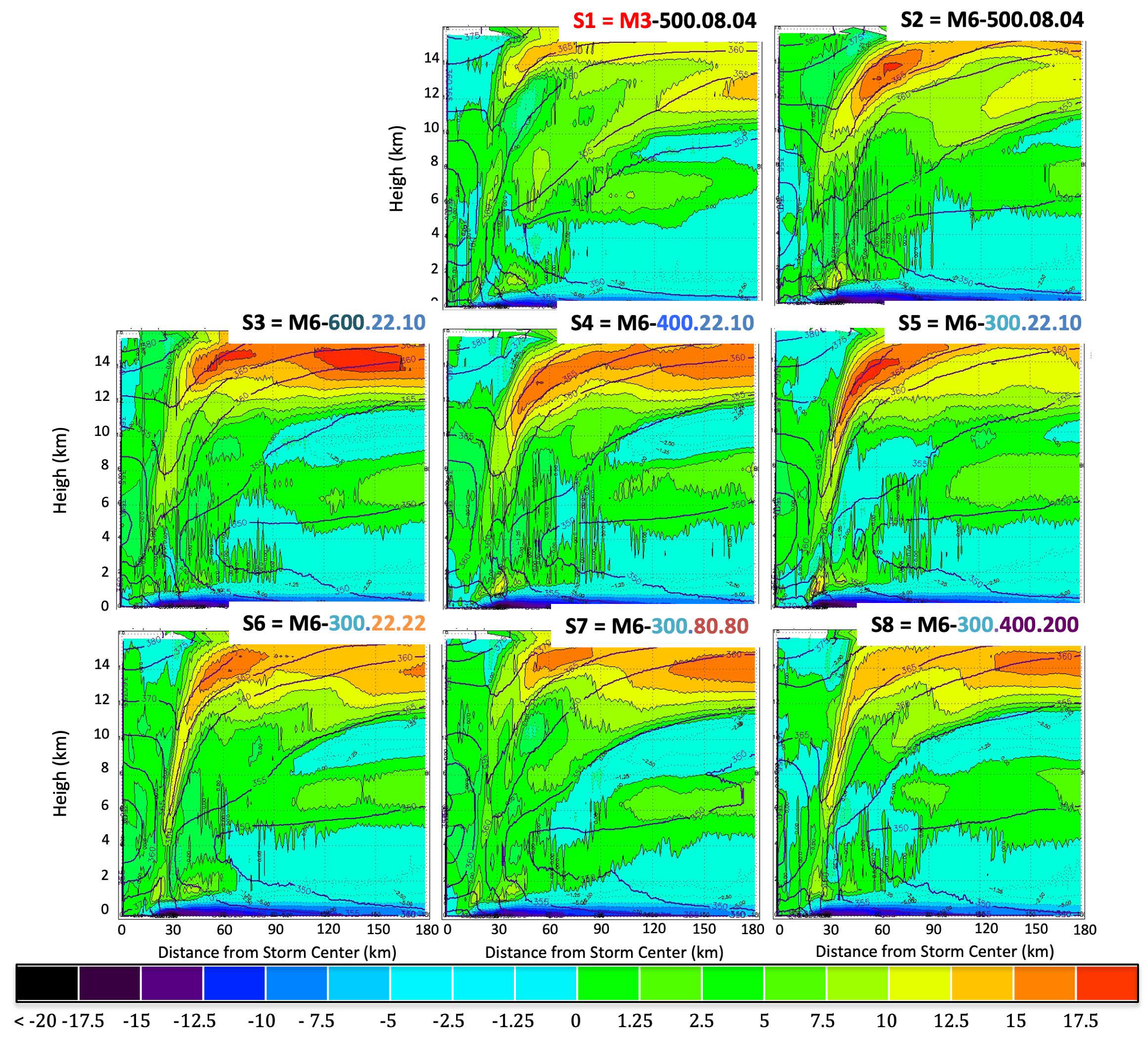
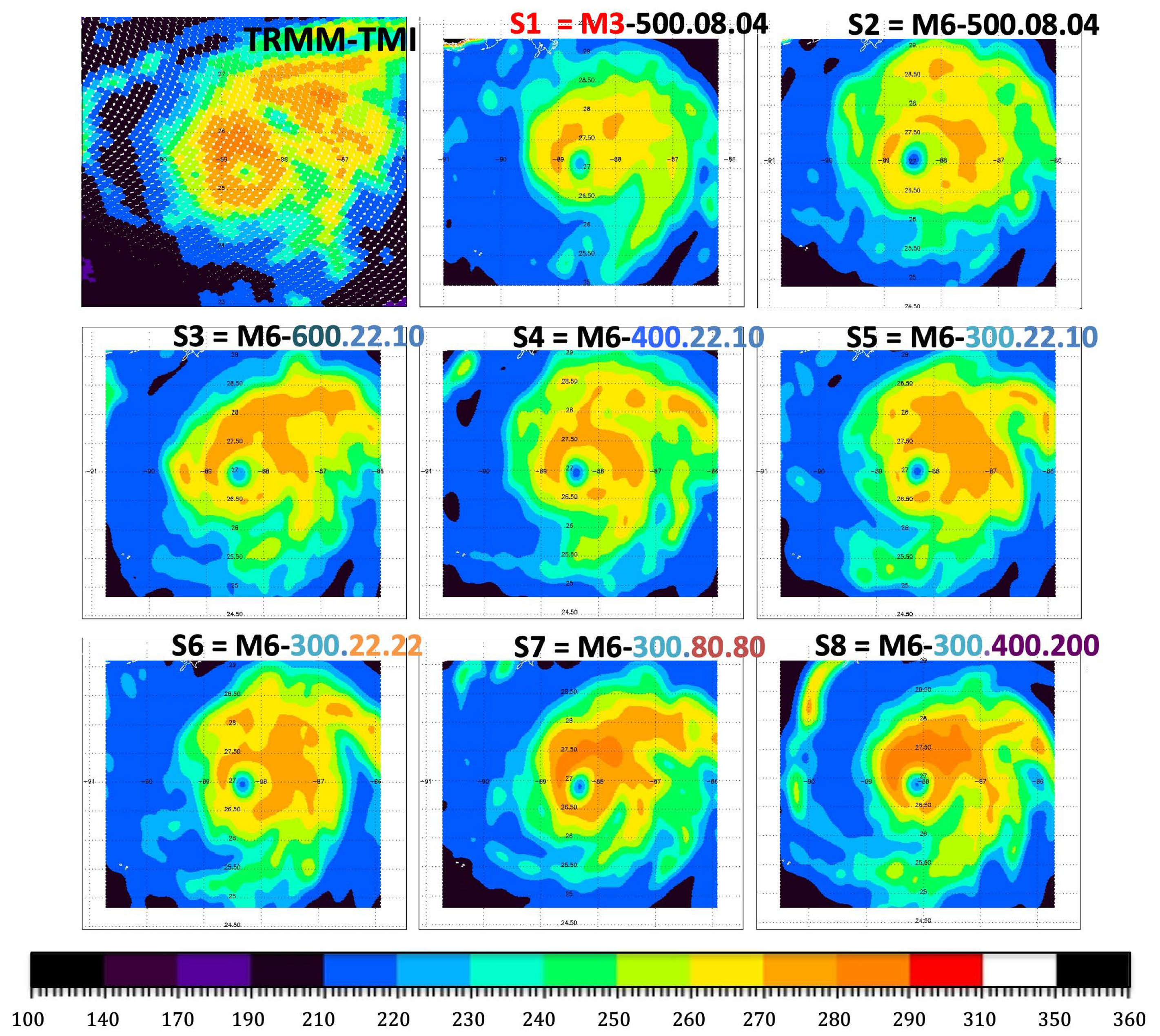