Spatio-Temporal Patterns of Mass Changes in Himalayan Glaciated Region from EOF Analyses of GRACE Data


CSIR-National Geophysical Research Institute, Hyderabad 500007, India
*
Author to whom correspondence should be addressed.
Remote Sens. 2021, 13(2), 265; https://doi.org/10.3390/rs13020265
Submission received: 1 November 2020
/
Revised: 16 December 2020
/
Accepted: 17 December 2020
/
Published: 14 January 2021
(This article belongs to the Special Issue Terrestrial Hydrology Using GRACE and GRACE-FO)
Abstract
:The nature of hydrological seasonality over the Himalayan Glaciated Region (HGR) is complex due to varied precipitation patterns. The present study attempts to exemplify the spatio-temporal variation of hydrological mass over the HGR using time-variable gravity from the Gravity Recovery and Climate Experiment (GRACE) satellite for the period of 2002–2016 on seasonal and interannual timescales. The mass signal derived from GRACE data is decomposed using empirical orthogonal functions (EOFs), allowing us to identify the three broad divisions of HGR, i.e., western, central, and eastern, based on the seasonal mass gain or loss that corresponds to prevailing climatic changes. Further, causative relationships between climatic variables and the EOF decomposed signals are explored using the Granger causality algorithm. It appears that a causal relationship exists between total precipitation and total water storage from GRACE. EOF modes also indicate certain regional anomalies such as the Karakoram mass gain, which represents ongoing snow accumulation. Our causality result suggests that the excessive snowfall in 2005–2008 has initiated this mass gain. However, as our results indicate, despite the dampening of snowfall rates after 2008, mass has been steadily increasing in the Karakorum, which is attributed to the flattening of the temperature anomaly curve and subsequent lower melting after 2008.
1. Introduction
The Himalaya holds one of the major concentrations of glaciers outside the poles [1]. These glaciers are a significant water source for major river basins such as the Ganga, Brahmaputra, Indus, Yangtze, Irrawaddy, etc. The melt-water released from them into the river basins during summer months maintains a healthy base flow and also serves as a major source of fresh water supply during the non-monsoon months for the millions of people living in these river basins. For these reasons, the monitoring of Himalayan glaciers is vital, as variations in melting or accumulation of these glaciers may lead to increased river flows, unseasonal flooding, overall sea-level rise [2], or drying-up of rivers. However, inaccessibility and difficult terrain make in situ observations difficult to install and maintain, so only a few glaciers have been monitored for more than a decade. The Himalayan region has diverse climatic regimes ranging from humid sub-tropical to cold semi-arid type. Spatially and temporally sparse records may not suffice in a scenario where the seasonality of accumulation/ablation, and consequently, the nature and magnitude of response to perturbation, varies [3,4]. Satellite-based methods, both optical and non-optical (e.g., [4,5]), having lengthier records, need to be monitored in such a situation. Optical satellite-based methods are used to estimate volume through mapping of the extent of the glacier and its thickness [6], but, in a few instances, persistent cloud cover may skew the results of seasonal snow cover extents [7,8]. This is particularly true for summer-accumulation type glaciers, where accumulation and ablation are not clearly demarcated [9]. It may be difficult to detect fragmented and isolated ice mass loss by the optical method, especially if the region falls in shadow or has an area less than image resolution [10]. A non-optical satellite method is mass derived from satellite gravity from Gravity Recovery and Climate Experiment (GRACE) and is a more direct means of calculating the mass balance. However, the spatial resolution is insufficient to independently monitor small regions [5,7], though it can provide a synoptic view of mass variability.
Various hydrological components such as groundwater, surface water, snow, and ice, as well as tectonic causes contribute a major part of surface/subsurface mass changes over time [11]. Hydrological mass exchange inside solid earth, its interaction with the atmosphere, and variation in this process over time can be amalgamated through time-varying gravity measurements/temporal gravity [12]. For a large glaciated region, seasonal mass accumulation and ablation is the largest contributor to the change in the basin/region wide temporal gravity field apart from smaller hydrological signals and tectonic signals, if any. We focus on spatio-temporal mass variability from time-varying GRACE satellite gravity data over the Himalayan Glaciated Region (HGR). It is likely that GRACE signals over the narrow HGR are influenced by signals from the non-glacial regions due to spatial smoothing of GRACE data [13]. It is possible to de-convolute the GRACE signal over HGR to separate out possible causative factors for variance and enable the differentiation of the glaciological signal from the surrounding hydrological and extraneous signals. Analyses are carried out over HGR as a whole and then a smaller sub-region of the western Himalaya. Empirical orthogonal functions (EOFs) are calculated and the resultant spatio-temporal patterns are compared with different hydrological factors such as rainfall, snowfall, and temperature to arrive at the glacial component of the total gravity signal. EOF analyses are often applied for localization of spatiotemporal signal, as well as being used as an alternative technique to enhance the GRACE signals [11,14,15]. However, EOFs are also used to de-convolute a signal into its components, as exemplified by de-Viron et al. (2006, 2008) [11,14] to separate the tectonic part from the total GRACE gravity anomaly. Establishing a cause-and-effect relationship between temporal gravity components and climatic variables such as precipitation, river discharges, snow accumulation, and temperature is an important part of the analysis. We utilized the Granger type of causality proposed by Granger (1969) [16], based on the definition proposed by Weiner (1956) [17], to establish the relationships between correlating variables. Initially meant for econometrics, this method is finding increasing application in hydrologic and climatologic attribution studies [18].
2. Study Area and Datasets
2.1. Study Area
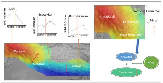
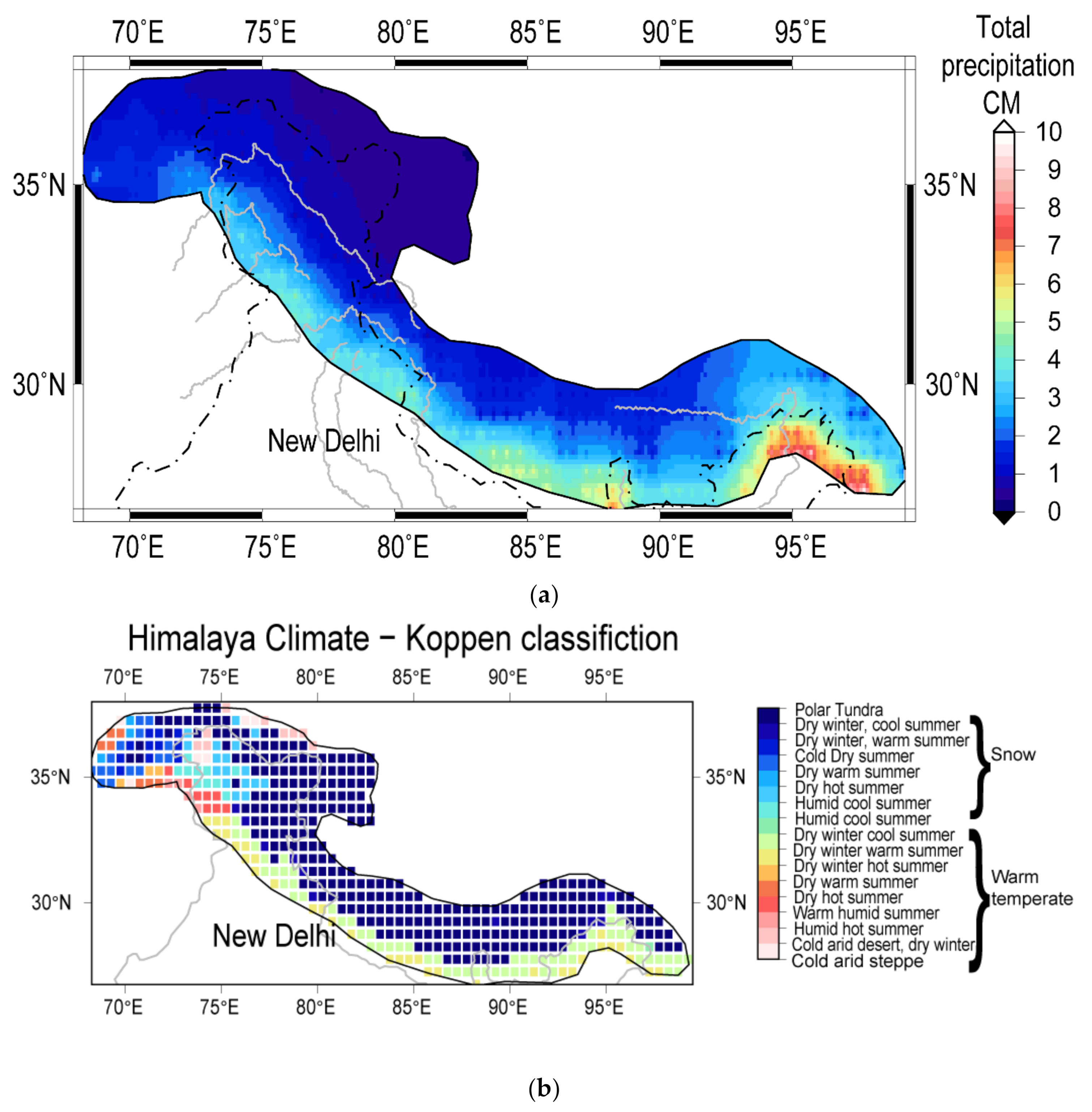
The Himalaya extends from the eastern syntaxis to the western syntaxis, comprising Hindukush, Karakoram, Kashmir Himalaya, Garhwal and Kumaon, Nepal, and the eastern Himalaya. The region extends from 69°E to 95°E and from 27°N to 37°N. It is 200–400 km wide and ~1500 m long, constituting parallel ranges which have varied climate, with an elevation ranging between 1000 m and 8000 m. It ranges on the Köppen scale from humid subtropical forest to alpine grassland to cold desert depending on the distribution of the precipitation mechanism and intensity. The lower ranges have a humid subtropical type of climate (Köppen Classification, [19], Figure 1b), the higher ranges are of alpine and tundra type, while regions like Karakoram, which receive less precipitation, are cold desert type. Generally, the lower-altitude eastern Himalayan regions are wetter. The influence of westerly–winter precipitation is dominant in the northwest and decreases towards the east and south, the majority of it being solid precipitation. The southwest summer monsoon shows maximum influence over the eastern part, and its intensity decreases westwards and northwards (Figure 1a). Köppen classification of climate in the Himalayan mountain ranges, extends from alpine grass land to cold desert and, humid sub-tropical climate in the lower reaches. Distribution of precipitation intensity influences the climate type, the lower altitude eastern Himalaya are wet, and at the western end, Karakoram ranges are cold desert type, in tune with the precipitation intensity (Figure 1).
There are approximately over 9000 Himalayan glaciers according to the inventory by the Geological Survey of India; although, other surveys project different numbers [20]. This is the largest concentration of glaciers outside the poles, with an average height of 4000 m above sea level and higher. The climatic conditions of these glaciers vary among different regions. Some recent studies indicate that the stability of western glaciers is mostly due to a higher percentage of solid precipitation and lower temperatures [3,4,6]. Figure 2 shows the GRACE-derived mass trend over HGR and surrounding regions. The Himalaya boundary and the traditional divisions and glacier locations within the Himalaya are plotted over the maps. For the present study, we consider the region bounded by the red line in Figure 2, which is larger than the Indian Himalaya boundary. This boundary is considered because glaciers lying outside the traditional boundaries contribute to the water budget of the Himalayan rivers.
2.2. Dataset
2.2.1. Time-Varying Gravity
Variation in the seasonal hydrological mass in response to accumulation and ablation patterns is estimated through time-variable gravity data. For regions with discontinuous glacier systems, this method could be more promising than methods based on satellite imagery, albeit with a compromise on spatial resolution [4]. Estimates in time-varying gravity are obtained for the period from January 2003 to December 2016 from the CSR RL 05 mascon solution in equivalent water height (EWH) format. The solutions are obtained from CSR (http://www.csr.utexas.edu/grace) at 0.5° grid spacing and at approximately a 30-day time interval [21]. The mascon solution is considered to have a better signal-to-noise ratio because it applies prior constraints while processing, and regularization constrains for this computation are derived from GRACE information only. Additional scaling, filtering as in the earlier CSR release, is not applied here, so the solutions are not biased towards a particular application and also, they do not have a visible stripe, as seen in the spherical harmonic (SH) solutions. The mascon solutions are corrected for Glacial Isostatic Adjustment (GIA) according to the model given by A et al. (2013) [22]. The algorithm is a 3-D visco-elastic model which incorporates past ice loading histories from ICE-5G [23] and 3D in-homogeneous visco-elastic response of the earth’s surface. These mascon solutions are suitable to monitor land ice mass changes [22]. GIA in HGR and its surrounding areas is very minimal, in the order of 1 mm/year, and has a negligible effect on mason solution, especially at the time scales (mostly seasonal) dealt with in this paper. Effect of GIA on the contemporary mass changes of the study area from each of the models and CSR solutions is discussed in detail in Supplementary Figure S1.
2.2.2. Climatic Variables
Climate data: Solid precipitation in the form of snowfall over the study area, air temperature, and ground snow cover in water equivalents (SWE) provided by the Global Land Data Assimilation System (GLDAS) is used in the present study. The data used are the 0.25° × 0.25° monthly outputs from Version 2.1 GLDAS NOAH 10 model, in area density units, i.e., kgm−2 for snowfall and SWE, and temperature in Kelvin. It is a global land surface parameter data assimilation system, which provides more reliable satellite—ground-truth-model hybrid data. The NOAH model is a land surface model (LSM) developed especially for climatology research and data assimilation systems [24]. The latest 2.1 version of the model uses observation-based climate forcing from MODIS, while being consistent with older versions of data. The monthly data are averaged from 3-h estimates and presented in area density units. Snowfall and SWE is converted to depth per grid in cm, i.e., equivalent to GRACE data units and gridded to 0.5° resolution.
Liquid precipitation: The TRMM Multi-Satellite Precipitation Analysis (TMPA 3B43 V7) data, available as monthly accumulated and gridded rainfall at 0.25° grid, are used in this study. It is a combined estimate of parameters from satellite data gathered by TRMM and ground truth data gathered by CAMS global gridded rain gauge data, and a global rain gauge product produced by the Global Precipitation Climatology Centre (GPCC) (http://disc.sci.gsfc.nasa.gov/precipitation/documentation/), which gives the best estimate of precipitation rate for each month, based on 3 hourly averages in mm/h units [25]. This particular product of TRMM is a combination of TRMM and other satellite data, along with in situ rain gauge measurement, and has the least Root Mean Square error when compared to available in situ data. which is further referred to in the document as ‘rainfall’.
EOFs of snowfall, rainfall, SWE, and seasonality are calculated from the data in cm/grid format. A normalized format of the cm/grid data is used for correlation and causality analysis. GRACE data is used as-is for EOF and seasonality calculation, and normalized for correlation and causality analysis.
3. Methodology
The objective of this paper is to decipher the contemporary glacier signal of GRACE data in Himalaya. Analysis of statistical modes, the culmination of statistical decomposition of the GRACE time series over this region, for physical significance is proposed as a method to accomplish this objective. Hypothesis: Lagged correlation between statistical modes and climatology variables is an indicator of causality, which is treated as a precursor to causality, and this hypothesis is tested with Granger causality analysis. Cause–effect, and thereby physical significance of a statistical mode, is established only when lagged correlation and Granger-causality both necessarily exist.
3.1. Statistical Decomposition: EOF
Time-variable gravity reflects the sum total of all the mass changes occurring due to time-dependent change in surface processes. At a given time, more than one process actively contributes to the gravity anomaly. Our objective is to separate each of these variables across space and time, analyze them, and separate out the part of the signal related to glacial mass change. EOF analysis is a prevalent technique for understanding the statistical pattern of spatio-temporal data, which was introduced to earth sciences by Lorentz (see Randal, Empirical orthogonal functions [26]). The basic principle of EOF is to decompose a centered stochastic process into a combination of linear orthogonal functions, also called basis functions, which are infinite for the continuous case, and finite and dimensionality-bound for the discrete case. EOFs of mass signal from the time-variable GRACE gravity field for the period 2002–2016 over the entire Himalaya is calculated. Data are first arranged as a spatio-temporal matrix, centered and detrended following the Toumazou and Cretaux (2001) [27] algorithm, and are decomposed into their constituent basis function, representing this spatio-temporal pattern as follows:
where is the pre-processed data matrix, i.e., an M-dimensional vector of time series N, and is centered, then the EOFs calculated for this set are the eigenvectors of its covariance matrix or . The eigen vectors of X, and thereby is defined as follows:
which is equal to
μ is the EOF explaining variation along the spatial dimension, and , the principal component (PC), explains variation along the temporal dimension. The eigen value of each eigenvector is the variance explained [28]. They are independent, mutually orthogonal basis functions and occur in associated pairs and in descending order of precedence; each such pair is called as a mode further in this paper. Modes occurring first having higher contribution variation are called lower modes and those occurring later with lower contribution to variation are called higher modes. Interpretation of each of these modes in terms of physical variables is possible [29].
Singular value decomposition (SVD) algorithm of MATLAB is employed for the calculation of eigen vectors, and is defined as
where is a vector, each of whose elements is the variance accounted for in the corresponding mode. The letter ‘k’ represents the number of total basis functions calculated and k = min (N,M). In SVD, each new calculated basis function is orthogonal to the previous one, and no transformation is required. Mutually uncorrelated orthogonal modes are possible only for a Gaussian process [27], and since the gravitational field is a multivariate Gaussian, independence of the modes is assured.
Post-processing of modes consists of scaling, normalization, and truncation of modes. Only those with a maximum contribution, significantly different from zero, i.e., upwards of 1%, are retained, and the rest are attributed to noise and truncated. The uniqueness of each mode in the SVD method ensures that a simple scree test is enough to truncate the modes. The eigen value corresponding to each mode is plotted in decreasing order; the plot resembles a cliff. All modes above the cliff bottom which contribute >1% of variance are retained and analyzed. In this paper, we discuss only those modes which we were able to interpret in terms of hydrology and glaciology.
3.2. Granger Causality
Granger causality is a statistical method developed by Granger (1969) [16] for testing and conforming directional causative relationships between variables, and it is used as a confirmation for correlation hypothesis. Henceforth, Granger causality refers to this method of causality quantification. The principle is based on persistence and predictability as necessary conditions, which means that if X and Y show persistent lagged correlation, then one variable can be predicted using the other. Granger causality can be stated as: ‘If X causes Y, the error of predicting future values of Y in a universe devoid of X is higher compared to a universe including X’. For a variable X to Granger-cause Y, a lagged correlation between X and Y is a prerequisite. Calculating causality is based on disproving the null hypothesis that X does not Granger-cause Y. A vector auto-regressive (VAR) model of Y using both X and Y and only Y is formulated, and F-statistic is calculated for these models. Let Y1 and Y2 be VAR models of Y at a lag L, where L is the maximum lag at which correlation exists between X and Y
A series of Y1 and Y2 models between lags [0, L] are constructed, and the most robust pair of models, say (Y1′ and Y2′), are selected based Bayesian Information criteria.
X is considered to cause Y if the F-statistic is greater than a critical value α. This relationship is unidirectional when lag between the variables exists, and there is a possibility for bidirectional causality or the existence of a feedback mechanism when there is no lag. This method is being applied increasingly to climatic studies, where attributing changes to climatic variables is necessary [18]. Mohkov et al. (2011) [30] used this method to establish bidirectional coupling between the El Niño Southern Oscillation (ENSO) and the strength of the Indian monsoon, while Kaufman et al. (2007) [31] investigated the effect of urbanization on precipitation.
4. Results
EOF modes of GRACE data are analyzed and compared with the climatic variables, namely, total precipitation, snowfall, and temperature, to arrive at a physical interpretation for these modes. Here, we discuss the modes which have a significant covariance, i.e., >1%, and correlate with climatic and hydrologic variables within the boundary of Himalaya discussed earlier. These results are used to form broad climatic divisions in the Himalaya.
4.1. Seasonality
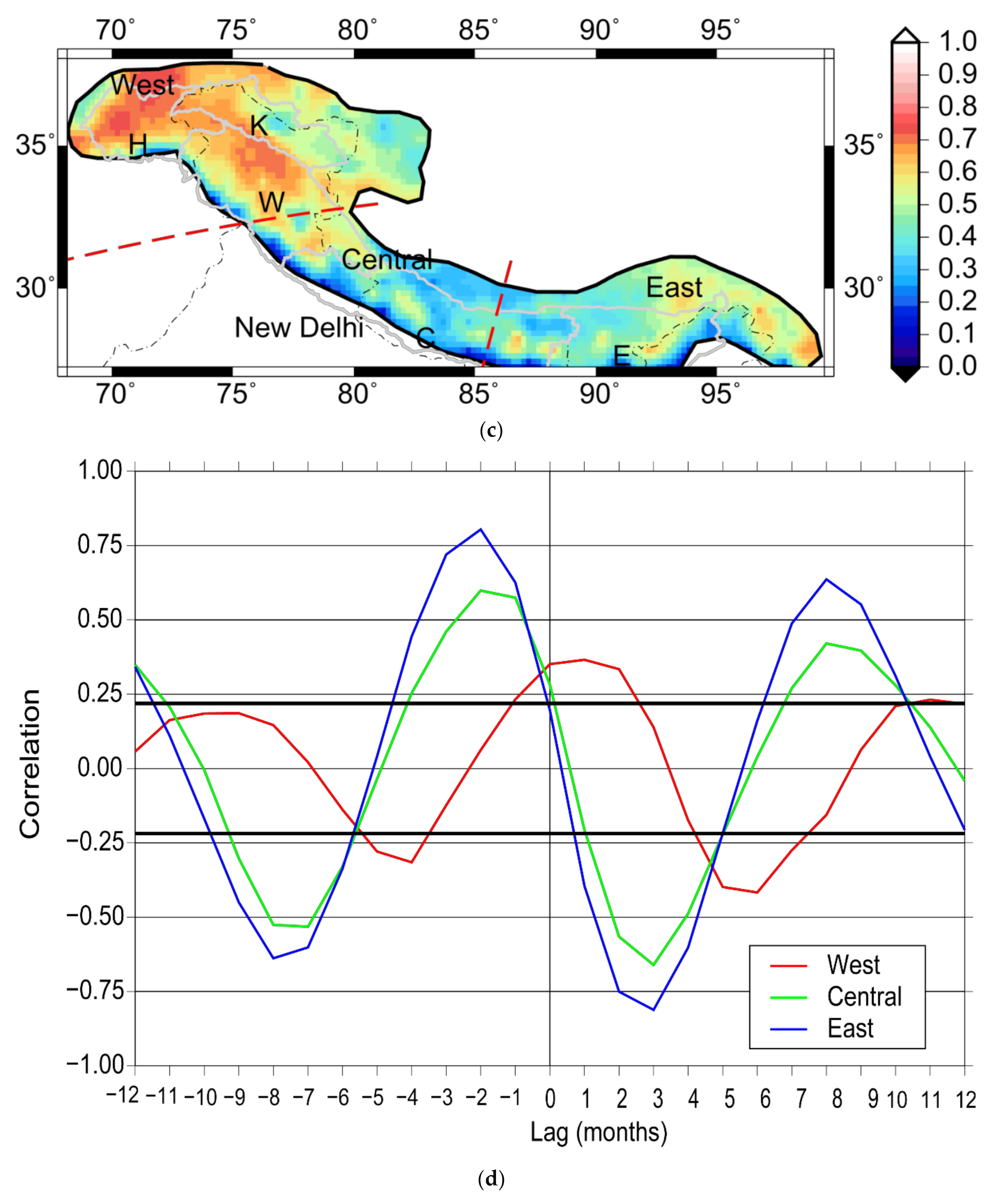
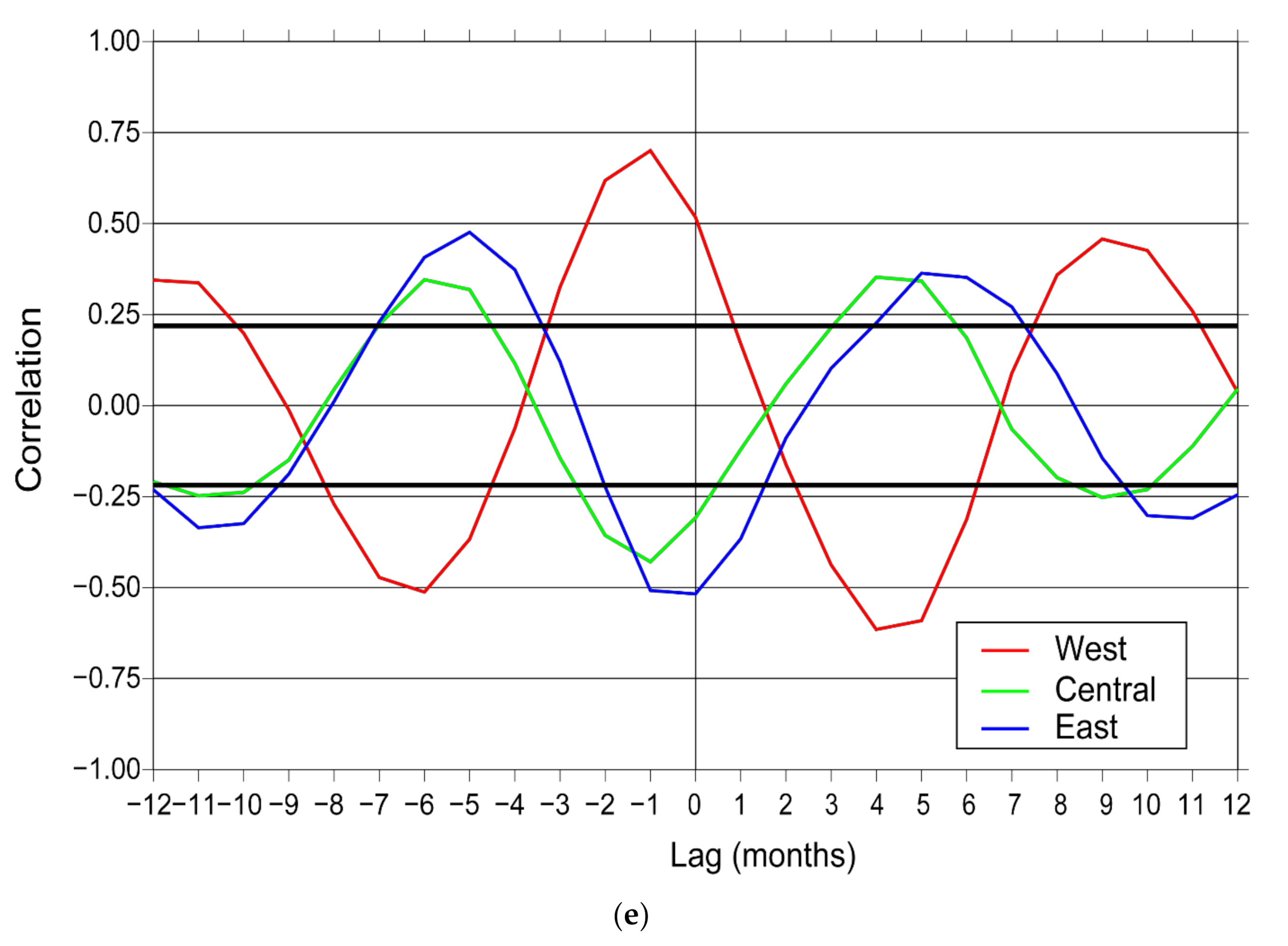
Spatio-temporal variation contributed by the first mode, constituting 71% of the variation in temporal gravity for the Himalaya, is shown in Figure 3a. The spatial part shows a gradual change in the sign and intensity of the amplitude from west to east. The western end is positive, and the eastern end is negative. The grid-wise cross-correlation of this mode with rainfall and snowfall are presented in Figure 3b,c. The data are corrected for autocorrelation effect, using the first difference and second difference of the normalized data before correlation is calculated. The correlograms (Figure 3b,c) show gradual change in the correlation of mode 1 of GRACE data with snowfall in the western region to rainfall in the eastern region. For a small part in the central area (between [75°E, 31°N] and [85°E, 26°N]) both snowfall and precipitation correlate partially with mass changes. Using this correlation result, we demarcate HGR into three broad regions depending on the dominant correlating variable, i.e., western (snowfall dominant), eastern (rainfall dominant), and central zone (which does not show a definitive relationship with snowfall and rainfall, but is rather a transition zone where two precipitation mechanisms are at play). A red line, shown in Figure 3b,c, marks the boundaries of the demarcated regions. The lagged correlation of area averaged time series of each of these regions with area averaged climatology is also calculated, where the climatology is ‘x’ variable, and the mode is ‘y’ variable. The results of this computation are shown in Figure 3d,e. Maximum correlation occurs at lags −1 and −2 months for ‘West’ and ‘East’, respectively, which implies that ‘x’ variable leads the ‘y’ variable, a precursor of a cause–effect relationship. A correlation of 0.75 at lag −1 is noticed in the eastern part, where rainfall dominates (Figure 3d), and correlation in the western part of the region in which snowfall dominates, is 0.62 at lag −1 (Figure 3e). Granger causality for mode 1, with the correlating climatic variables, i.e., rainfall and snowfall, for each of the regions demarcated in Figure 3b,c is calculated and tabulated in Table 1.
For the calculation, the mode is considered as Y variable, and climatology is the X variable in Equations (4)–(6). For the western region, F-statistic of mode vs. snowfall is above critical value, and for eastern region, F-statistic of mode vs. rainfall is above the critical value. For the central region, the F-statistics of mode vs. rainfall and mode vs. snowfall are greater than their respective critical values.
Monthly averages for the study period, i.e., seasonality of these divisions from GRACE gravity and climatic variables, i.e., rainfall and snowfall, are calculated, and are expected to show distinctly different variability for the three regions. Distinct accumulation–ablation patterns can be discerned from the GRACE seasonality graph (Figure 4a), i.e., post-monsoon-accumulation/summer-ablation type in the eastern Himalaya; a mixed type, i.e., post-monsoon- and winter-accumulation/summer-ablation type in the central Himalaya; and summer- and early-monsoon-accumulation/winter-ablation type in the western Himalaya. Climatic variables (Figure 4b) emphasize the distinctive accumulation mechanisms at play across the Himalaya. The western region shows a snowfall-specific accumulation occurring in February to March and picking up again post-monsoon, with a negligible monsoon rainfall compared to winter snow precipitation. The central region shows two distinct accumulation seasons, winter snowfall precipitation and monsoon rainfall. For the eastern region, rainfall and snowfall seasons are close together, and the resulting hydrological and glaciological accumulation manifests as a single summer-accumulation/winter-ablation season.
4.2. Interannual Variability
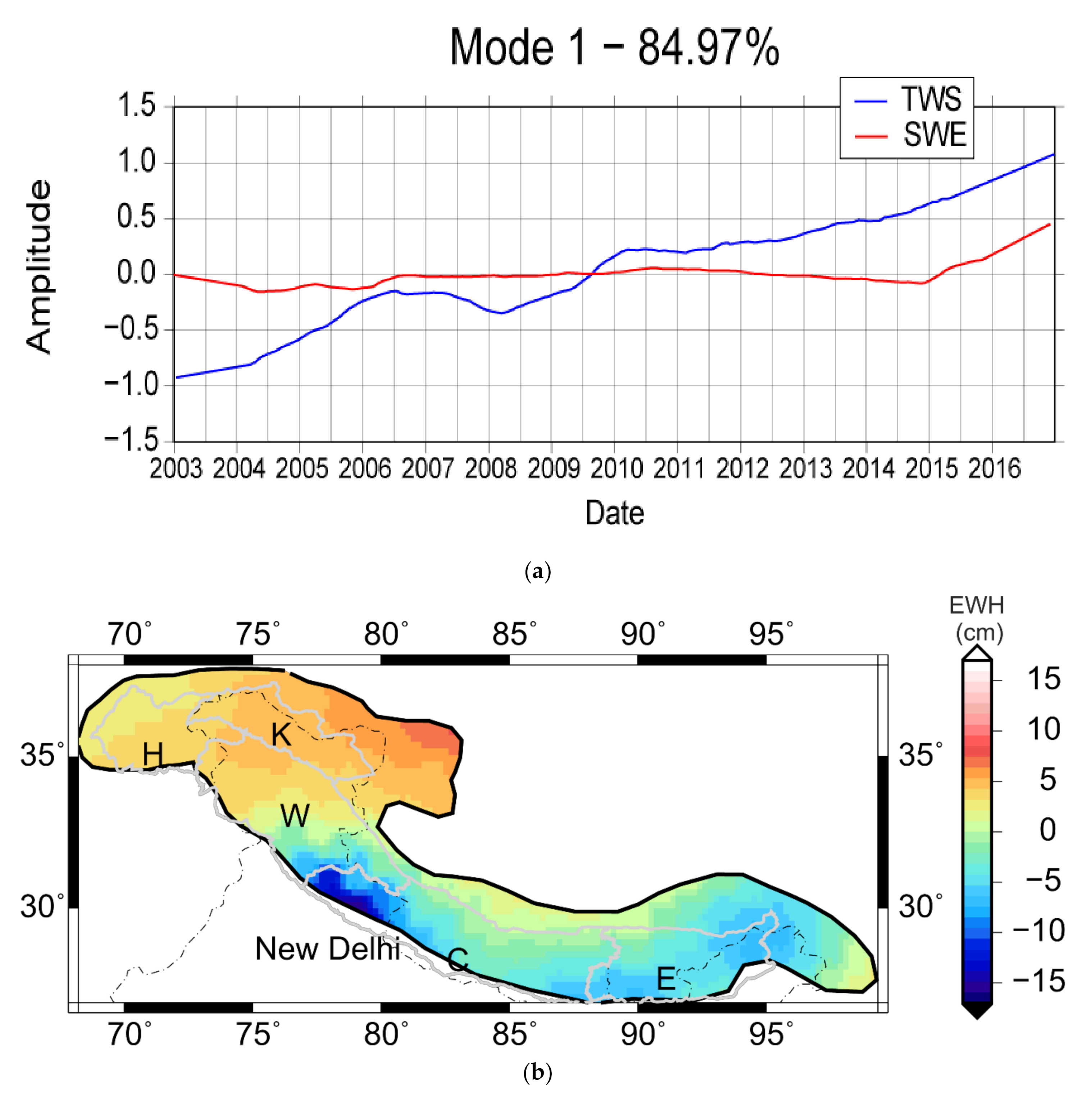
We analyze the spatial variation of the interannual part of the GRACE time series and its climatic connection at an interannual scale. The seasonal-removed time-series for each grid was calculated by fitting and removing the seasonal sinusoid, and the EOF of this timeseries is calculated and correlated with climatic variables. The 1st EOF mode of this data shows 84% of variability (Figure 5a), and appears to reflect the trend of mass change as captured by GRACE across the Himalaya (Figure 2). This mode shows that the western part of the Himalaya has been gaining mass at different rates during the study period, and the central and eastern parts have been losing mass at nearly the same rate. Rapid mass gain has occurred in the western Himalaya for 2003–2007 and again for 2009–2010, and thereafter, a stable mass change with a very small gain. The association with climatic signals with this mass change pattern was investigated, and a good correlation 0.7 at 0 Lag with ground snow cover is found (Figure 5b). The specific mechanism for the mass change pattern in the western Himalaya is discussed in Section 4.3.
4.3. Spatio-Temporal Variations in the Western Himalaya
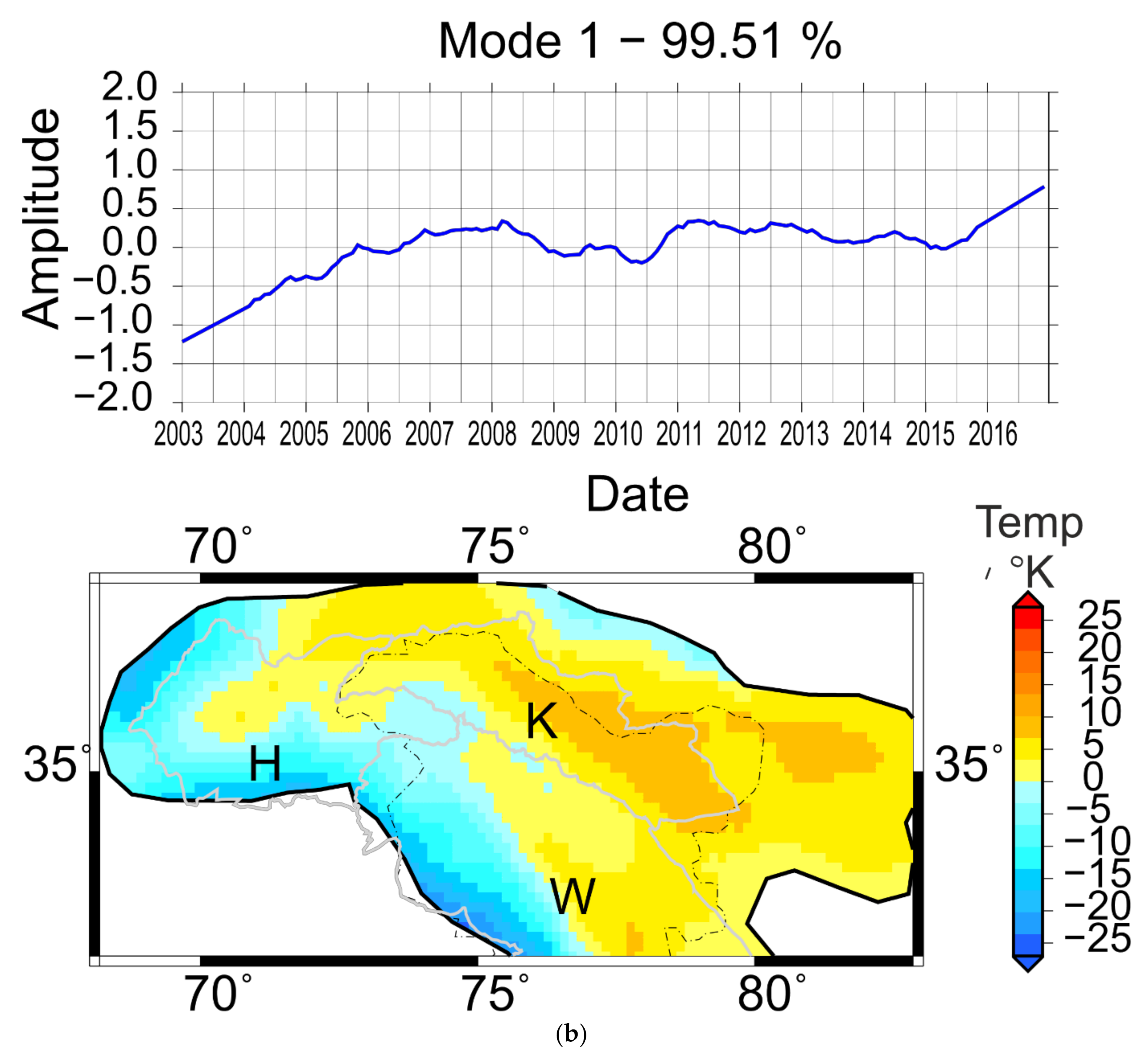
As noted in Section 4.2, the western Himalaya shows a distinct increase in mass change pattern at an interannual scale. ‘Western Himalaya’ refers to the boundary demarcated in Figure 3b,c above 32° latitude. The EOF Mode1 of the western Himalaya at an interannual scale region accounts for 56% of the variability (Figure 6a). The regional differences are evident within the area, which showed up as a single unit in the earlier EOFs (Figure 3 and Figure 5). However, the major part of the area shows a mass increase, as against a small portion to the south, which shows a decrease. The time series and spatial pattern of Mode 1 for air temperature (Figure 6b) is similar to the time series of GRACE Mode 1 (Figure 6a), for the most part. The EOF of snow cover (SWE), has a cyclic trend up to the year 2014, and the spatial pattern shows high snow cover within Karakorum Himalaya. A steady mass gain, centered in the Karakorum region, is depicted, except for a few years where there was a slight mass loss. EOFs for this region indicate the Karakoram high anomaly, i.e., mass gain of the Hindukush and Karakoram glaciers, was initiated due to cumulative ground snow cover up to 2007.
The correlation between GRACE Mode 1 with SWE and temperature are 0.5 and 0.69, both at a zero lag (Table 2). It is also noticed that the F-value of causality analyses for both the climatic variables is greater than the critical value (Table 2), but the F-value for mode vs. air temperature is higher than that of mode vs. SWE.
5. Discussion
Summarizing the methodology, EOF, i.e., a statistical decomposition method for separating Gaussian data into its basis components of time variable gravity from GRACE, is calculated. The basic idea was to analyze the modes and pick-up glacial mass balance part of the signal using a combination of causality and correlation, in other words, assign a physical meaning to statistical modes.
5.1. A Summary of the EOF Analysis
Temporal changes in gravity over any region represent a sum total of changes in the physical process active in that region. In the Himalaya, the active physical processes are mostly on the surface, such as seasonal snowfall and snowmelt, glacier accumulation, and temporary surface water storage, and the source for them is precipitation.
At the outset, it was observed that spatially variable seasonality is found to be the dominant mode (Mode 1, Figure 3a), implying varied mass accumulation patterns across the Himalaya. In the variable represented by Mode 1, changes in the western part are opposite in sense to those in the eastern part, i.e., for time series of the variable represented by this mode, the western part will be negative when the rest is positive, and vice versa. Supposing this mode represents seasonal snow accumulation, then from Figure 3a we can infer that the western part is winter accumulation type and the east is summer accumulation type, with the central part having a transitional nature. Heterogeneity in correlating variables expressed in this mode is used to demarcate the Himalaya into three broad regions (Figure 3b,c), representing three different types of accumulation–ablation patterns occurring across the Himalaya. The 1st mode also represents snow accumulation and melt seasons depending on seasonal precipitation, as confirmed by grid-wise cross-correlation of this mode with rainfall and snowfall (Figure 3b,c). Causality and seasonality analysis from climatological variables also attest the heterogeneous accumulation–ablation patterns. The lagged correlation suggests that mode 1 represents total hydrological accumulation as a result of precipitation, i.e., both rainfall and snowfall, with the western part of the mode representing the seasonal snowpack. This lagged correlation of data also suggests a cause–effect relationship, which we confirm using Granger causality. However, such good correlation is also found between physically uncorrelated variables which have similar periodicity and are normalized to lie within the same range. This ambiguity is solved with Granger causality. Interpretation of the causality calculation is as follows: F-statistic is the measure of ‘if there is a significant relationship between two populations’; F-value above a critical value implies rejection of the null hypothesis that the populations are not related. Variables registering larger F-values cause mode 1 more than others. Thus, from Table 1 we see that, for the eastern part, rainfall is the causative factor for variance in time-variable gravity as its F-value is above the critical value, and snowfall is the causative factor in the western part. In the central region, both rainfall and snowfall register an F-value larger than the critical value, the F-value for snowfall being much larger than that for rainfall, establishing the mixed precipitation mechanism of the central region. Solid precipitation, i.e., snowfall, is dominant in the western region, and from the seasonality of the mode it can be seen that it is mostly winter precipitation, western disturbances being the main cause. Liquid precipitation, i.e., rainfall, is the dominating factor in the eastern end, the southwest summer monsoon being the source. The central region is a combination where both precipitation mechanisms are at play and their strengths differ from year to year, as evident from the correlation and seasonality analysis (Figure 3c and Figure 4). Hence the division made based on hydroclimatic nature (Figure 3b,c) is further supported by GRACE observations and demarcates HGR into three broad regions depending on the dominant correlating variable, i.e., western (snowfall dominant), eastern (rainfall dominant), and central zone (which does not show a definitive relationship with snowfall and rainfall, but is rather a transition zone where two precipitation mechanisms are at play). Thus, three varied climatic regimes for the Himalaya are established, and the boundaries of the climatic regions are demarcated. The behavior of glaciers in these regions would also differ in accordance with the dominant precipitation type in the region. The mass changes in the eastern region are due to liquid precipitation from summer monsoon; snow/ice storage in this region would be less than in the central and western regions, reflecting the precipitation pattern (Figure 3b,c and Figure 4, Table 1). This region is particularly vulnerable to extreme climatic events like cloudburst and drought, which cause more lasting impacts. The western Himalaya, with large snow accumulation, would respond more slowly to precipitation pattern perturbation, while the eastern region responds faster, and the central regions lie somewhere in between. In the central part, even though snowfall from monsoons could differ with change in precipitation intensity, it can be compensated by the advent of winter snow (Figure 4). Spatio-temporal variability at an interannual scale depicts the trend of mass change occurring in the Himalaya (Figure 5a) is really the variability of snow storage (Figure 5b), especially in the western and eastern parts. The spatial pattern in Figure 5a shows a significant negative signal in the central part, which has its origin outside the Himalaya, which is the influence of Ganga basin hydrology on the dynamics of the Himalaya. Owing to the differences in precipitation mechanisms, individual analysis of these three regions could give a better estimation of the glacial health of the Himalaya. The western region is dominated by westerly winds, and snowfall is the dominant mode of precipitation, mostly occurring from January to May (Figure 4). This season facilitates cumulative accumulation due to lower temperatures. Snowfall decreases southward and eastward, hence the shift to negative trends [32]. For the western region, we see an accelerated accumulation up to 2007, followed by a decrease up to 2008, and again accumulation up to 2010, stabilizing later. The remaining part registers accelerated depletion up to 2007, and accumulation from 2005 to 2008, stabilizing later. The entire Himalayan region shows stability after 2010 (Figure 3a). The western part is analyzed separately to further understand the dynamics.
External dynamics: Many earlier workers (e.g., [33]) have pointed out the influence of processes happening outside Himalayas on the GRACE gravity signal in Himalaya and the subsequent uncertainty in glaciological estimates. Region wide hydrological balance [34] considering the full GRACE signal do have a scope of contamination from non-hydrological/glaciological signals, given the uplift history of the region [35]. EOFs, as mentioned earlier, are orthogonal basis functions of the data, and each mode carries unique information in descending order of precedence, and hence each contributing variable to the total variance can be separated. Accordingly, it was hypothesized that lower modes will relate to processes happening inside the boundary and will be hydrological/glaciological signals of our study area, and higher modes will be the influence of external factors on Himalaya.
It is pertinent to mention that amplitude and time period of mass variability between tectonic and seasonal mass signals are considerably different. Tectonic signals (uplift) would be in the order of a few mm (~5 mm/year; in the higher Himalaya) which is comparatively very small to the seasonal and inter-annual signals of tens of cm of EWH. Further, along axis variation in the Himalayan uplift is small and can give rise to differences in the observed seasonal mass signals. The major influence could be from the continuous depletion of Terrestrial Water Storage in the Ganga basin [33]. External influences were defined based on the position of the center of anomaly in the spatial pattern of the EOF, i.e., if the center of the anomaly lies inside our boundary, the EOF pertains to dynamics within the Himalaya. Based on this assumption, the first mode (Figure 3) depicts the seasonal variation within the Himalaya, as a result of precipitation patterns within the Himalaya, at an interannual scale (Figure 5), there may still a small part of influence from the Ganga basin. However, considering the CSR mascon data [21] used and EOF analysis localizes the spatiotemporal signal [14], leakage of outside signals would be minimal. Moreover, EOF signal is validated with in situ glacier mass balance data (Figure 7) in the subsequent sections for assessment. Higher modes do contain information related to external influence over Himalaya. In the second, third, and fourth modes, the spatial patterns have anomaly centers outside our boundary, and the modes do not correlate with any climatic or hydrologic variables of the Himalaya, hence these modes could relate to the influence of various processes outside the Himalaya on the GRACE signal for the Himalaya. A detailed analysis of the higher modes is presented in Supplementary Figure S2.
GIA
Upliftment histories in the Tibet–Himalaya region are spatially varied [36], and southern Tibet has a higher rate of upliftment [37]. GRACE has been useful for understanding Tibet upliftment histories [38]. However, the current GIA models for Tibet, in the absence of ice loading histories, are calculated from mantle viscosity models [39,40,41]. GRACE CSR mascon data used in this study is already correct for GIA (using coefficients from A et al. 2013 [20]), but we have compared three widely extant GIA models against raw GRACE mascons (i.e., containing GIA) to gauge the effect of GIA on the total region. For this aim, an area comprising Tibet, the Himalaya, and the northern Indian plains is considered. All the three models show that the spatial variability in GIA for the current study area is on the order 0.5–1 mm/year, which is much less than the GRACE error limit. An EOF analysis of the GIA corrected vs. raw mascon data reveals no change in the data distribution of the major modes, implying the GIA effect on the climatic/hydrological/glaciological signals from the Himalaya is minimal and can be filtered using the EOF analysis. A detailed description of the GIA effect on this study area is presented in Supplementary Figure S1. Hence, the major mode does represent the mass changes occurring due to processes happening inside the Himalaya, as a result of climatic processes only.
5.2. Western Himalaya
The western region is distinct from the rest of the Himalaya in terms of glacier behavior. The glacial response to climatic changes is highly lagged or disharmonious with climatic changes in the Karakoram region, which Bhambri et al. (2016) [42] attribute to high concentrations of surge type glaciers, as surge activity interferes with response, whereas Gardelle at al. (2013) [43] attribute Karakorum mass gain to surging activity of glaciers. An average increase of 0.1% in the area of the Karakorum glaciers was reported, and individual glacier retreat is lower than that of rest of the Himalaya [44], and also more fragmentation of glaciers [43] was reported. A region wide mass balance study for Pamir Hindukush and Karakorum shows positive mass balance concentrated to the Karakorum region [43]. Higher amounts of NDSI (Normalized Difference Snow Index) were reported [45]. Kapnick et al. (2014) [46] reported positive temperature anomalies and non-significant snowfall gain in Karakorum, and resilience of seasonal cycles. Winter precipitation in the western Himalaya occurring, mainly due to westerly winds as a causative factor for mass changes in this region, has been established so far [47].
The results from EOF and causality indicate that mass gain in Karakorum is due to glacier mass gain as a result of favorable temperatures, reflecting the conclusions from in situ data and model analysis by various workers stated above. Analyzing mass changes at an interannual scale gives us an idea of the long-term behavior of a particular region. From correlation and causality analysis of Mode 1 of the western region against climatic variables, it is understood that the lagged relationship between the mode, air temperature, and snowfall translated to cause and effect, yet air temperature has a bigger role in stabilizing mass, as seen from the F-statistics (Table 2). A moderately steady mass gain, centered in the Karakorum region, is depicted, except for a few years, where there was a slight mass loss. EOFs for this region indicate that the Karakoram high anomaly, i.e., mass gain of the Hindukush and Karakoram glaciers, was initiated due to cumulative ground snow cover up to 2007 as a result of high precipitation, depicted by the EOF of SWE. However, as the results indicate, in spite of the dampening of snow cover rates after 2008, mass has been steadily increasing; which is attributed to lowering and stabilizing of temperature in this region after 2008. The results imply that mass changes depicted by Mode1 (Figure 6a) are more a result of change in temperature than snowfall. On observing the time series (Figure 6), it is understood that the initial mass gain was triggered because of a higher snowfall, and sustained later due to the lower temperatures which inhibit melting.
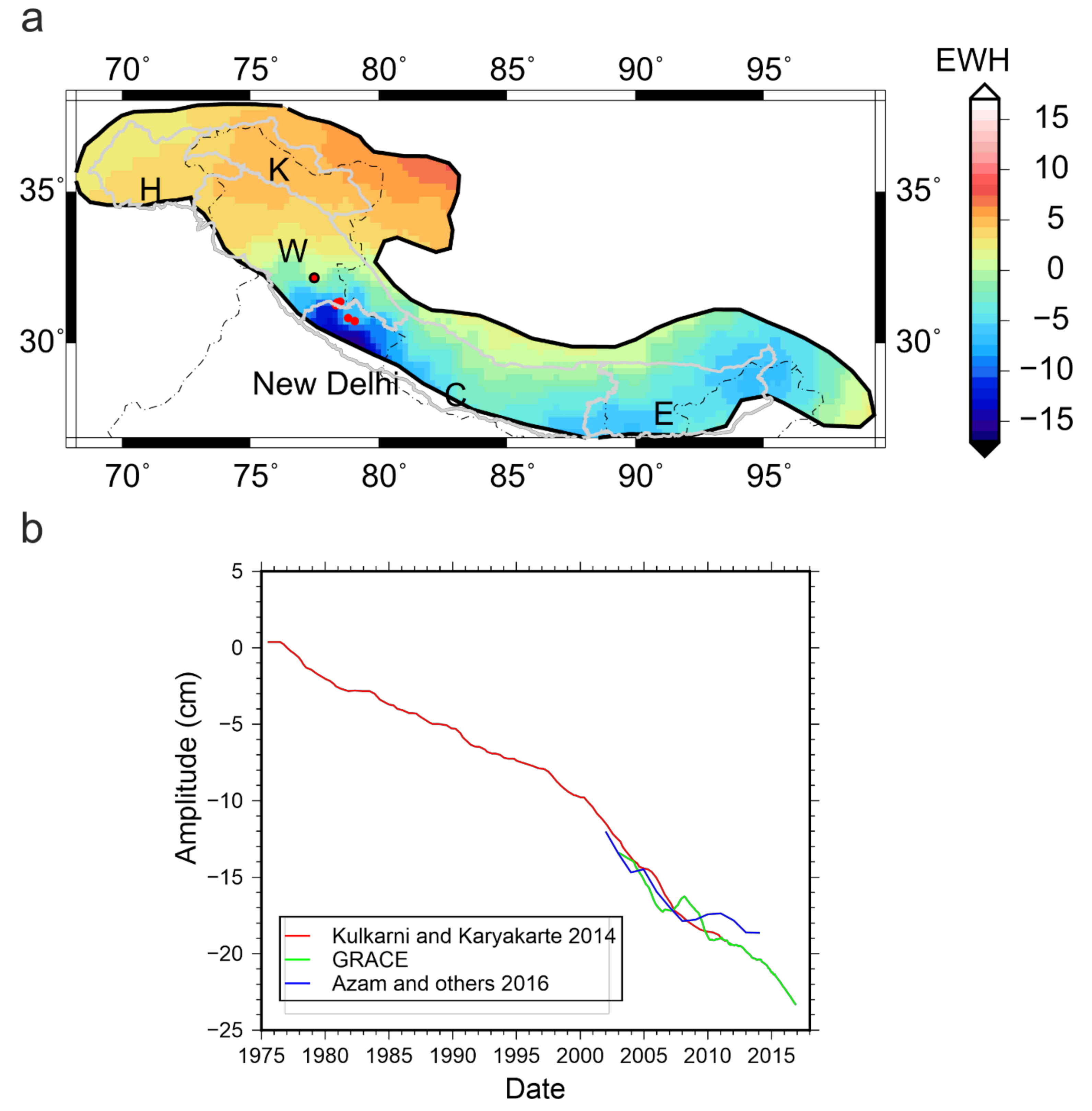
In-situ vs GRACE: A common problem with in situ measurements as stated by each of the works referenced at the start of Section 5.2 is the lack of continuous measurements exceeding five years. Data from a few glaciers which have overlapping records with the GRACE time-period are compared, although they are not from the Karakorum region. Figure 7a depicts the glacier locations from Kulkarni and Karyakarte (2014), and Azam et al. (2016) [20,48], which are confined to the central Himalaya, plotted on interannual mode 1 spatial distribution (Figure 5b). The first interannual mode (Figure 5), i.e., convolution of the spatial and temporal parts of the mode from GRACE for the glacier locations, is compared with in situ observations from the papers. The compounded cumulative mass balance for all the glaciers from Kulkarni and Karyakarte (2014) [21], i.e., Gara, Gor Garang, Shaune Garang, Chota Sigri, Dokrani, Hamtah, and Chorabari, and cumulative yearly mass balance of Chhota Shigri, Azam et al. (2016) [48] are time series that are compared (Figure 7b). For both the cases (Figure 7b) it is seen that the general trend of in situ data and GRACE closely match, and in the case of Kulkarni and Karyakte (2014) [20], GRACE provides an extension to in situ mass balance calculation. This is in spite of GRACE averaging mass variation of the total grid area and having more information than the individual in situ point measurement. For the existing published in situ time series, the mode does represent actual glacier mass variation. By extension, it can be said that major mode of the GRACE EOF at interannual scale does provide an insight into spatial distribution of Glacier mass balance intensities. However more studies incorporating spatially extensive in situ data are called for.
6. Conclusions
Diversity in mass change across the Himalaya is demonstrated using EOFs of GRACE temporal-gravity over the entire region. The spatio-temporal variance patterns over the Himalaya using EOFs of mass signal derived from GRACE temporal gravity, and variables causing the major part of the variance in mass are investigated using lagged correlation, and causal relationships are presented. We were able to show the spatial and temporal heterogeneity of seasonal accumulation–ablation patterns existing within the Himalaya. This heterogeneity is used to demarcate three regions of the Himalaya: Western, central, and eastern. The precipitation regimes and orientation of glaciers change from west to east, thereby affecting the mass balance regimes and trend. Precipitation in the Himalaya is mainly from the southwest summer monsoon, which is mostly liquid precipitation, i.e., rainfall, and western disturbances which are mostly solid precipitation i.e., snowfall [49]. The dominance of these two factors is spatially variable [32], ranging from westerly, i.e., winter, snowfall in the northwest, comprising Hindukush and Karakoram, to summer monsoon rainfall and snowfall in the eastern Himalaya, the central region being a transition zone between the two. Earlier workers like Kääb et al. (2012) and Bolch et al. (2012) [1,4], have considered demarcations across the Himalaya to facilitate analysis of changes in glacier status, climate changes, etc. Based on our analysis of time-variable gravity from GRACE and the evidence we have for the difference in precipitation regimes across the Himalaya (Figure 3, Table 1), the demarcation into three regions, i.e., western, central, and eastern is appropriate. The seasonality of these three divisions is examined. Monthly averages of these divisions from GRACE gravity and climatic variables, i.e., rainfall and snowfall, are calculated and plotted, and are expected to show distinctly different graphs for the three regions. Distinct accumulation–ablation patterns are seen for GRACE (Figure 4a), i.e., post-monsoon-accumulation/summer-ablation type in the eastern Himalaya; a mixed type, i.e., post-monsoon- and winter-accumulation/summer-ablation type in the central Himalaya; and summer- and early-monsoon-accumulation/winter-ablation type in the western Himalaya. Climatic variables (Figure 4b) emphasize the distinctive accumulation mechanisms at play across the Himalaya. The western region shows a snowfall-specific accumulation occurring in February to March and picking up again post-monsoon, with a negligible monsoon rainfall compared to winter snow precipitation. The central region shows two distinct accumulation seasons, winter snowfall precipitation and monsoon rainfall. For the eastern region, rainfall and snowfall seasons are close together, and the resulting hydrological and glaciological accumulation manifests as a single summer-accumulation/winter-ablation season. Tiwari et al. (2009) and Matsuo and Heiki (2010) [7,33] pointed out the influence of the Ganga basin low signal over the Himalaya for GRACE estimates. In spite of taking care to eliminate the grids nearer the Ganga basin from the study area, the effect of this signal (Supplementary Figure S2, Figure 5) is encountered in this work. EOF analysis effectively separates the contribution of external factors into a separate mode and, in this case, we are able to isolate uncontaminated parts of the signal and the variation solely depends on changes in snow and ice and are free from surrounding influence (Figure 3, Mode 1). Persistent questions, such as removing the influence of the Ganga basin low on the GRACE signal from the Himalaya, are thus addressed, and it’s similar to other studies carried out using EOF [11]. The GIA and tectonic uplift effects on surface mass changes in HGR is also too small to be a statistically significant factor in EOF analysis (Supplementary Figure S1) for the comparison of along axis variation. A causal relationship between modes of temporal gravity and climatic variables is proposed. At an interannual scale, GRACE mass changes reflect stored snow, which if coupled with optimum temperature, has the potential to become glacier ice. The western region registers a different pattern compared to the rest. EOFs for this region indicates the Karakoram high anomaly, i.e., mass gain of the Hindukush and Karakoram glaciers. This mass gain was initiated due to cumulative ground snow cover up to 2007 as a result of high precipitation, depicted by the EOF of SWE. However, as our results indicate, in spite of the dampening of snow cover rates after 2008, mass has been steadily increasing; this is attributed to the lowering and stabilizing of temperature in this region after 2008. Causality analysis indicates that SWE and, more so, air temperature play a role in mass change for this region. For glaciated regions like the western Himalaya, although snowfall is required to accumulate glacier mass, what stabilizes the ablation rates is lower temperatures, which facilitate storage of ice and conversion of fresh snow to glacier ice, as seen in the western Himalayan region. The non-monsoonal winter precipitation is considered to be a major source of mass anomalies [46]. The initial ground snow cover pre-2007 is sustained due to the lowering of temperatures and, post-2014, lowering snow cover does not lower the mass change in western Himalaya, as lower temperatures continue to sustain the snows and aid in converting it to glacial ice. The results for the western Himalaya reflect the results from various other studies in that region, especially for the Karakorum range.
Supplementary Materials
The following are available online at https://www.mdpi.com/2072-4292/13/2/265/s1, Figure S1: GIA calculated from models and CSR given grids (a) ICE—6G model (b) CSR-mascon (c) Wahr 2000 model., Figure S2: GRACE—lesser modes of Himalaya at seasonal removed time scale a. Mode2 b. Mode3 c. Mode4.
Author Contributions
Conceptualization, V.M.T.; Methodology, H.M. and V.M.T.; Software, H.M.; Formal Analysis, H.M. and V.M.T.; Writing-Original Draft Preparation, H.M.; Writing-Review & Editing, V.M.T. and H.M.; Supervision, V.M.T. All authors have read and agreed to the published version of the manuscript.
Funding
This research received no external funding.
Data Availability Statement
Data is available through http://www.csr.utexas.edu/grace; and NOAA websites.
Acknowledgments
This work is done under a UGC-JRF fellowship to H.M. and DST GRACE Project. We also thank the organizers of the IGS 2015 symposium for providing the opportunity to present our work. We also benefited from discussions with Etienne Berthier. We appreciate M. Ravi Kumar for his help with GIA calculations. Data is available through http://www.csr.utexas.edu/grace; and NOAA websites.
Conflicts of Interest
The authors declare no conflict of interest.
References
- Bolch, T.; Kulkarni, A.; Kääb, A.; Huggel, C.; Paul, F.; Cogley, J.G.; Frey, H.; Kargel, J.S.; Fujita, K.; Scheel, M.; et al. The state and fate of Himalayan glaciers. Science 2012, 336, 310–334. [Google Scholar] [CrossRef] [PubMed] [Green Version]
- Immerzeel, W.W.; Pellicciotti, F.; Bierkens, M.P.F. Rising river flows throughout the twenty-first century in two Himalayan glacierized watersheds NGEO. Nat. Geosci. 2013, 6, 742–745. [Google Scholar] [CrossRef]
- Fujita, K.; Nuimura, T. Spatially heterogeneous wastage of Himalayan glaciers. Proc. Natl. Acad. Sci. USA 2011, 108, 14011–14014. [Google Scholar] [CrossRef] [PubMed] [Green Version]
- Kääb, A.; Berthier, E.; Nuth, C.; Gardelle, J.; Arnaud, Y. Contrasting patterns of early twenty-first-century glacier mass change in the Himalayas. Nat. Lett. 2012, 488, 495–498. [Google Scholar] [CrossRef] [PubMed]
- Gardner, A.S.; Moholdt, G.; Cogley, J.G.; Wouters, B. A reconciled estimate of glacier contributions to sea level rise: 2003 to 2009. Science 2013, 340, 852–857. [Google Scholar] [CrossRef] [PubMed] [Green Version]
- Gardelle, J.; Berthier, E.; Arnaud, Y. Slight mass gain of Karakoram glaciers in the early twenty-first century. Nat. Geosci. 2012, 5, 322–325. [Google Scholar] [CrossRef]
- Matsuo, K.; Heiki, K. Time-variable ice loss in Asian high mountains from satellite gravimetry. EPS Lett. 2010, 290, 30–36. [Google Scholar] [CrossRef]
- Prajka, J.; Pepe, M.; Rampini, A.; Rossi, S.; Bloschl, G. A regional snow-line method for estimating snow cover from MODIS during cloud cover. J. Hydrol. 2010, 381, 203–212. [Google Scholar] [CrossRef]
- Fujita, K. Effect of precipitation seasonality on climatic sensitivity on glacier mass balance. EPS Lett. 2008, 276, 14–19. [Google Scholar] [CrossRef]
- Kulkarni, A.V.; Bahuguna, I.M.; Rathore, B.P.; Singh, S.K.; Randhawa, S.S.; Sood, R.K.; Dhar, S. Glacial retreat in Himalaya using Remote sensing satellite data. Curr. Sci. 2007, 92, 69–74. [Google Scholar] [CrossRef]
- De Viron, O.; Panet, I.; Diamante, M. Extracting low frequency climate signal from GRACE data. Electron. Earth 2006, 1, 9–14. [Google Scholar]
- Wahr, J.; Molenaar, M.; Bryan, F. Time variability of the earth’s gravity field: Hydrological and oceanic effects and their possible detection using GRACE. J. Geophys. Res. 1998, 103, 30205–30229. [Google Scholar] [CrossRef]
- Landerer, F.W.; Swenson, S.C. Accuracy of scaled GRACE terrestrial water storage estimates. Water Resour. Res. 2012, 48. [Google Scholar] [CrossRef]
- De Viron, O.; Panet, I.; Mikhailov, V.; Van Camp, M.; Diamaent, M. Retrieving earthquake signature in Grace Gravity solutions. Geophys. J. Int. 2008, 174, 14–20. [Google Scholar] [CrossRef] [Green Version]
- Wouters, B.; Schrama, E.J.O. Improved accuracy of GRACE gravity solutions through empirical orthogonal function filtering of spherical harmonics. Geophys. Res. Lett. 2007, 34, L23711. [Google Scholar] [CrossRef] [Green Version]
- Granger, C.W.J. Investigating causal relations by econometric models and cross-spectral methods. Econometrica 1969, 37, 424–438. [Google Scholar] [CrossRef]
- Weiner, N. The theory of prediction. In Modern Mathematics for Engineers; Beckenback, E.F., Ed.; Series 1; McGraw-Hill: New York, NY, USA, 1956. [Google Scholar]
- Attanasio, A.; Passini, A.; Triaca, U. Granger causality analyses for climatic attribution. Atmos. Clim. Sci. 2013, 3, 515–522. [Google Scholar] [CrossRef] [Green Version]
- Kottek, M.; Grieser, J.; Beck, C.; Rudolf, B.; Rubel, F. World Map of the Köppen-Geiger climate classification updated. Meteorol. Z. 2006, 5, 259–263. [Google Scholar] [CrossRef]
- Kulkarni, A.V.; Karyakarte, Y. Observed changes in Himalayan Glaciers. Curr. Sci. 2014, 106, 25. [Google Scholar]
- Save, H.; Bettadpur, S.; Tapley, B.D. High resolution CSR GRACE RL05 mascons. J. Geophys. Res. Solid Earth 2016, 121, 7547–7569. [Google Scholar] [CrossRef]
- Geruo, A.; Wahr, J.; Zhong, S. Computations of the viscoelastic response of a 3-D compressible earth to surface loading: An application to glacial isostatic adjustment in Antarctica and Canada. Geophys. J. Int. 2013, 192, 557–572. [Google Scholar] [CrossRef]
- Peltier, W.R. Global glacial isostasy and the surface of the ice-age Earth: The ICE-5G (VM2) model and Grace. Ann. Rev. Earth Planet. Sci. 2004, 32, 111–149. [Google Scholar] [CrossRef]
- Rodell, M.; Houser, P.R.; Jambor, U.; Gottschalck, J.; Mitchell, K.; Meng, C.-J.; Arsenault, K.; Cosgrove, B.; Radakovich, J.; Bosilovich, M.; et al. The global land data assimilation system. Am. Meteorol. Soc. 2004, 85, 381–394. [Google Scholar] [CrossRef] [Green Version]
- Bolvin, D.T.; Huffman, G.J. Transition of 3B42/3B43 Research Product from Monthly to Climatological Calibration/Adjustment. 2015. Available online: https://gpm.nasa.gov/sites/default/files/document_files/3B42_3B43_TMPA_restart.pdf (accessed on 28 August 2020).
- Randall David, A. Empirical orthogonal functions. In Department of Atmospheric Sciences; Colorado State University: Fort Collins, CO, USA, January 2003. [Google Scholar]
- Toumazou, V.; Creteaux, J.-F. Using a Lancos eigen solver in the computation of Empirical orthogonal functions. Am. Meteorol. Soc. 2001, 219, 1243–1250. [Google Scholar]
- North, G.; Bell Thomas, L.; Cahalan Robert, F. Sampling errors in the estimation of Empirical Orthogonal functions. Am. Meteorol. Soc. 1982, 10, 699–706. [Google Scholar] [CrossRef]
- Forootan, E.; Kursche, J. Separation of global time-variable gravity signals into maximally independent components. J. Geod. 2012, 86, 477–497. [Google Scholar] [CrossRef]
- Mohkov, I.I.; Smirnov, D.; Nakonechny, P.I.; Kozlenko, S.S.; Seleznev, E.P.; Kurths, J. Alternating mutual influence of El Niño/Southern oscillation and Indian monsoon. Geophys. Res. Lett. 2011, 38. [Google Scholar] [CrossRef] [Green Version]
- Kaufmann, R.K.; Seto, K.C.; Schneider, A.; Liu, Z.; Zhou, L.; Wang, W. Climate response to rapid urban growth: Evidence of a human-induced precipitation deficit. J. Clim. 2007, 20, 2299–2306. [Google Scholar] [CrossRef]
- Bookhagen, B.; Burbank, D.W. Towards a complete hydrological budget: Spatiotemporal distribution of snowfall and rainfall and their impact on river discharge. J. Geophs. Res. 2010, 115. [Google Scholar] [CrossRef] [Green Version]
- Tiwari, V.M.; Wahr, J.; Swenson, S. Dwindling groundwater resources in Northern India from satellite gravity observations. Geophys. Res. Lett. 2009, 36, L18401. [Google Scholar] [CrossRef] [Green Version]
- Moiwo, J.P.; Yang, Y.; Tao, F.; Lu, W.; Han, S. Water storage change in the Himalayas from the Gravity Recovery and Climate Experiment (GRACE) and an empirical climate model. WRR 2011, 47, W07521. [Google Scholar] [CrossRef] [Green Version]
- Harrison, T.M.; Copeland, P.; Kidd, W.S.F.; Yin, A. Raising Tibet. Science 1999, 255, 1663. [Google Scholar] [CrossRef] [PubMed] [Green Version]
- Wang, C.; Zhao, X.; Liu, Z.; Lippert Peter, C.; Graham Stephan, A.; Coe Robert, S.; Yi, H.; Zhu, L.; Liu, S.; Li, Y. Constraints on the early uplift history of the Tibetan Plateau. Proc. Natl. Acad. Sci. USA 2008, 105, 4987–4992. [Google Scholar] [CrossRef] [PubMed] [Green Version]
- Xu, C.; Liu, J.; Song, C.; Jiang, W.; Shi, C. GPS measurements of present-day uplift in the Southern Tibet. Lett. Earth Planets Space 2000, 52, 735–739. [Google Scholar] [CrossRef] [Green Version]
- Jiao, J.; Zhang, Y.; Yin, P.; Zhang, K.; Wang, Y.; Bilker-Koivula, M. Changing Moho Beneath the Tibetan plateau revealed by GRACE observations. J. Geophys. Res. Solid Earth 2019, 124. [Google Scholar] [CrossRef]
- Paulson, A.; Zhong, S.; Wahr, J. Inference of mantle viscosity from GRACE and relative sea level data. Geophys. J. Int. 2007, 171, 497–508. [Google Scholar] [CrossRef] [Green Version]
- Stuhne, G.R.; Peltier, W.R. Reconciling the ICE-6G_C reconstruction of glacial chronology with ice sheet dynamics: The cases of Greenland and Antarctica. J. Geophys. Res. Earth Surf. 2015, 120, 1–25. [Google Scholar] [CrossRef] [Green Version]
- Wahr, J.; Wingham, D.; Bentely, C. A method of combining ICESat and GRACE satellite data to constrain Antarctic mass balance. J. Geophys. Res. 2000, 105, 16279–16294. [Google Scholar] [CrossRef]
- Bhambri, R.; Hewitt, K.; Kawishwar, P.; Pratap, B. Surge-type and surge-modified glaciers in the Karakoram. Sci. Rep. 2016, 7, 15391. [Google Scholar] [CrossRef]
- Gardelle, J.; Berthier, E.; Arnaud, Y.; Kääb, A. Region-wide glacier mass balances over the Pamir-Karakoram-Himalaya during 1999–2011. Cryosphere 2013, 7, 1263–1286. [Google Scholar] [CrossRef] [Green Version]
- Bahuguna, I.M.; Rathore, B.P.; Brahmbhatt, R.; Sharma, M.; Dhar Sunil, S.; Randhawa, S.S.; Kumar, K.; Romshoo, S.; Shah, R.D.; Ganjoo, R.K.; et al. Are the Himalayan glaciers retreating? Curr. Sci. 2014, 10, 1008–1013. [Google Scholar]
- Xiao, X.; Moore, B., III; Qin, X.; Shen, Z.; Boles, S. Large-scale observations of alpine snow and ice cover in Asia: Using multi-temporal vegetation sensor data. Int. J. Remote Sens. 2002, 23, 2213–2228. [Google Scholar] [CrossRef] [Green Version]
- Kapnick Sarah, B.; Delworth Thomas, L.; Ashfaq, M.; Malyshev, S.; Milly, P.C.D. Snowfall less sensitive to warming in Karakoram than in Himalayas due to a unique seasonal cycle. Nat. Geosci. 2014, 7, 834–840. [Google Scholar] [CrossRef]
- Dimri, A.P.; Niyogi, D.; Barros, A.P.; Ridley, J.; Mohanty, U.C.; Yasunari, T.; Sikka, D.R. Western Disturbances: A review. Rev. Geophys. 2015, 53, 225–246. [Google Scholar] [CrossRef]
- Azam, M.F.; Ramanathan, A.L.; Wagnon, P.; Vincent, C.; Linda, A.; Berthier, E.; Sharma, P.; Mandal, A.; Angchuk, T.; Singh, V.B.; et al. Meteorological conditions, seasonal and annual mass balances of Chhota Shigri Glacier, western Himalaya, India. Ann. Glaciol. 2016, 57, 328–338. [Google Scholar] [CrossRef] [Green Version]
- Bohmer, J. General climatic controls and topo climatic variation in central High Asia. Boreas 2006, 35, 279–295. [Google Scholar] [CrossRef]
Figure 1.
(a) Mean total precipitation for the period 2002–2017 (b) Köppen Climate classification from Kottek and others, 2006. Index for letters in the code: P = Polar, T = Tundra, D = Dry, w = winter, W = Warm, H = humid, h = hot, s = summer, c = cool, C = cold a = arid, d = desert, S = steppe.
Figure 1.
(a) Mean total precipitation for the period 2002–2017 (b) Köppen Climate classification from Kottek and others, 2006. Index for letters in the code: P = Polar, T = Tundra, D = Dry, w = winter, W = Warm, H = humid, h = hot, s = summer, c = cool, C = cold a = arid, d = desert, S = steppe.

Figure 2.
GRACE (Gravity Recovery and Climate Experiment) mass trend over the Himalayan Glaciated Region (HGR) and the surrounding region. Glaciers are represented as white dots (data source: World Glacier Monitoring Service, Boulder, CO, USA), the Himalaya boundary in grey, and the modified boundary used in this paper in red.
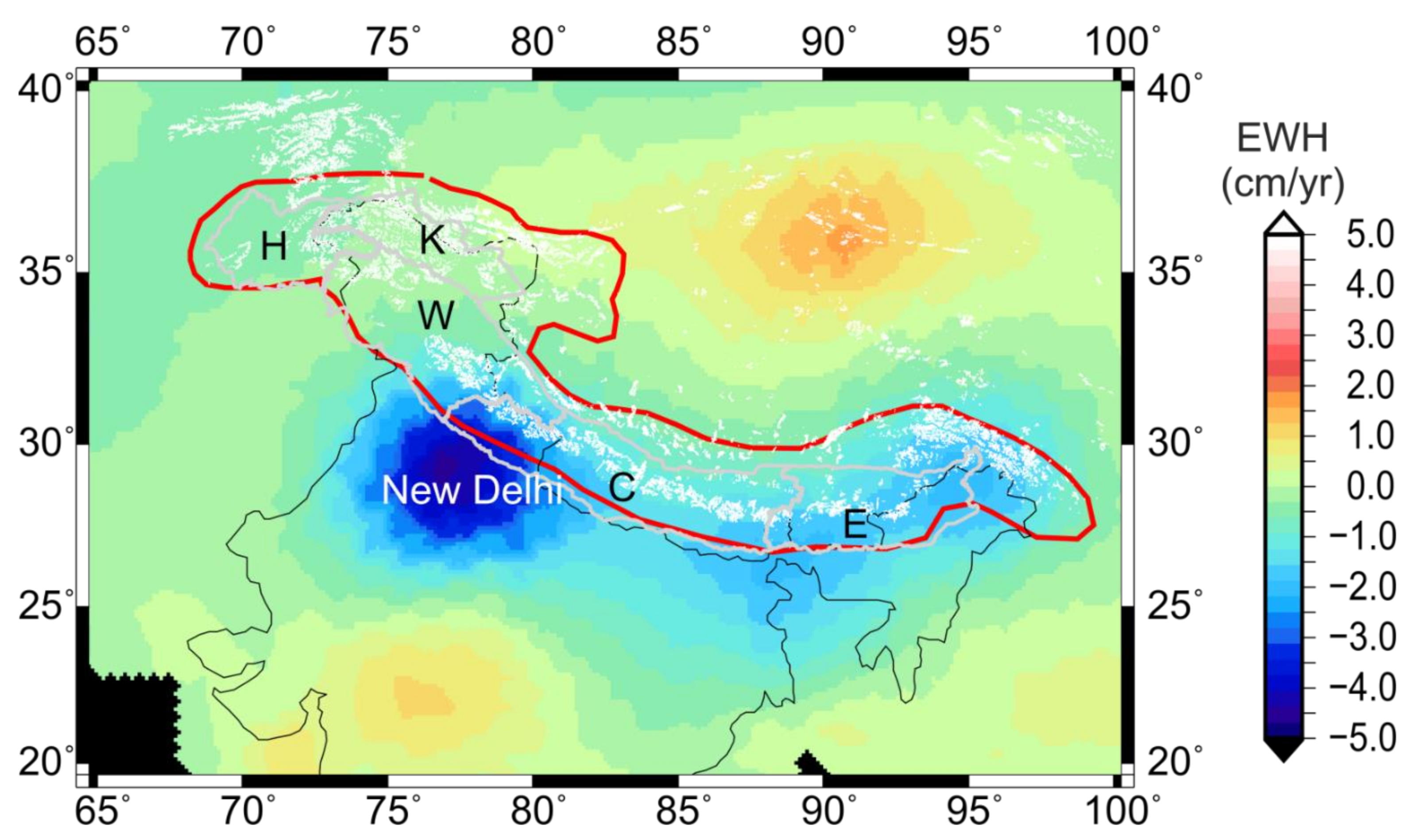
Figure 3.
Seasonal signal Mode 1 of Himalaya and its interpretation. (a) Empirical orthogonal functions (EOF) Mode 1 of Himalaya. (b) Grid-wise correlation of mode vs. rainfall. (c) Grid-wise correlation of mode vs. snowfall. (d,e) Cross correlations of the three regions demarcated and marked in red against rainfall and snowfall, respectively.
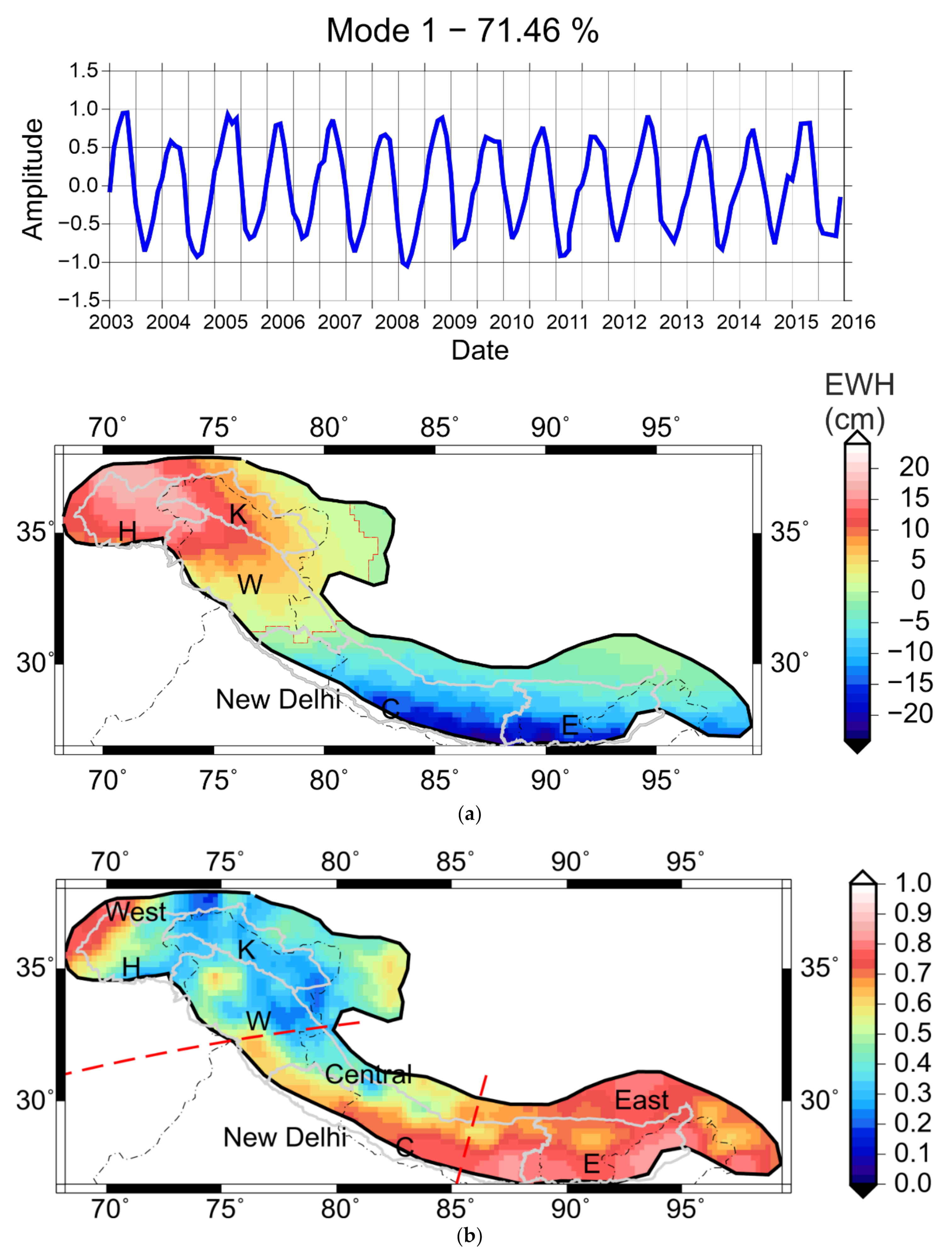


Figure 4.
Seasonality of mass change across the western, central and eastern regions. Left panel (a) is the seasonality of GRACE data and right panel (b) is of rainfall (dotted line) and snowfall (dashed line). Rainfall and snowfall are in cm. In each panel (i, ii, iii) is the seasonality for west central and east Himalaya regions, as marked in Figure 3b,c.
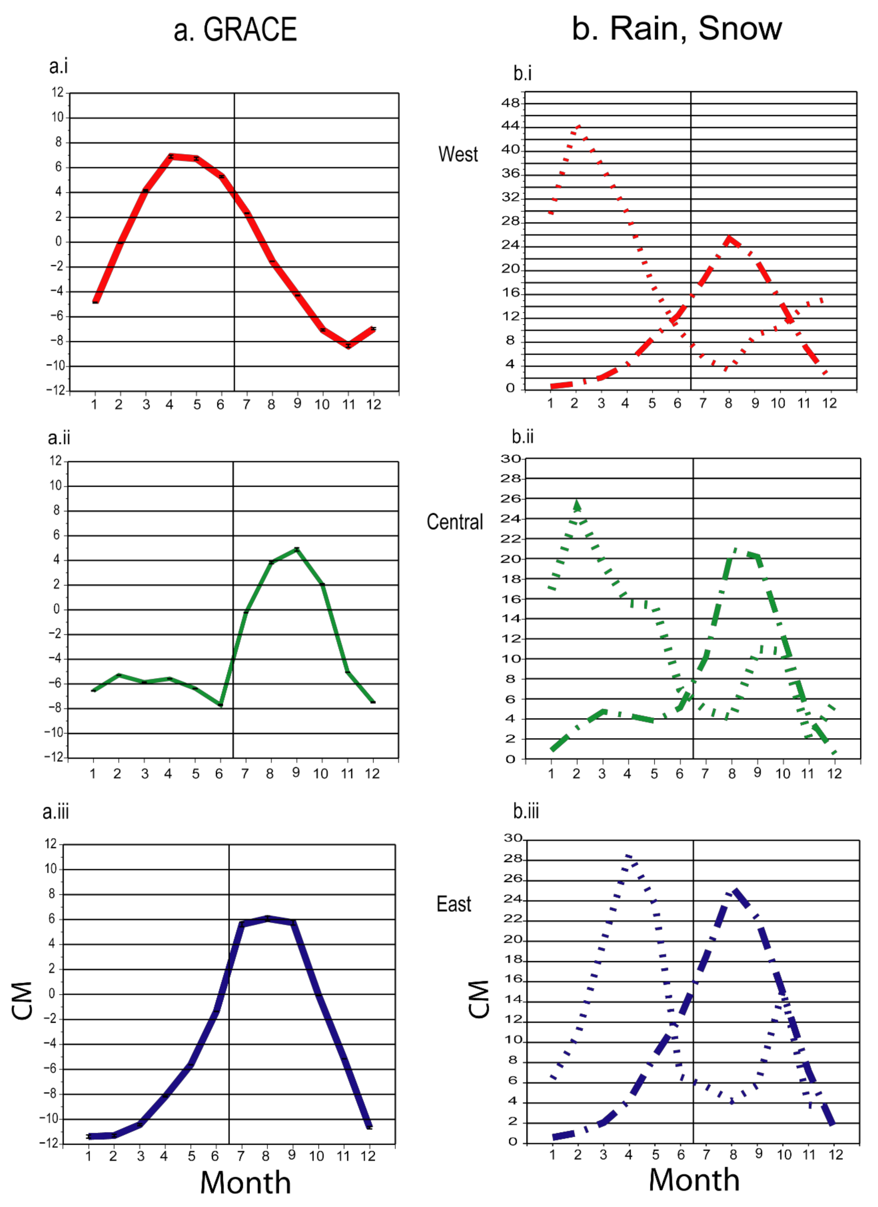
Figure 5.
Spatio-temporal variation of the interannual part of GRACE time series. (a) Timeseries of Mode 1 and snow cover in water equivalents (SWE). (b) Mode1 EOF spatial pattern. (c) Cross-correlation of Mode 1 against snowfall and SWE.
Figure 5.
Spatio-temporal variation of the interannual part of GRACE time series. (a) Timeseries of Mode 1 and snow cover in water equivalents (SWE). (b) Mode1 EOF spatial pattern. (c) Cross-correlation of Mode 1 against snowfall and SWE.

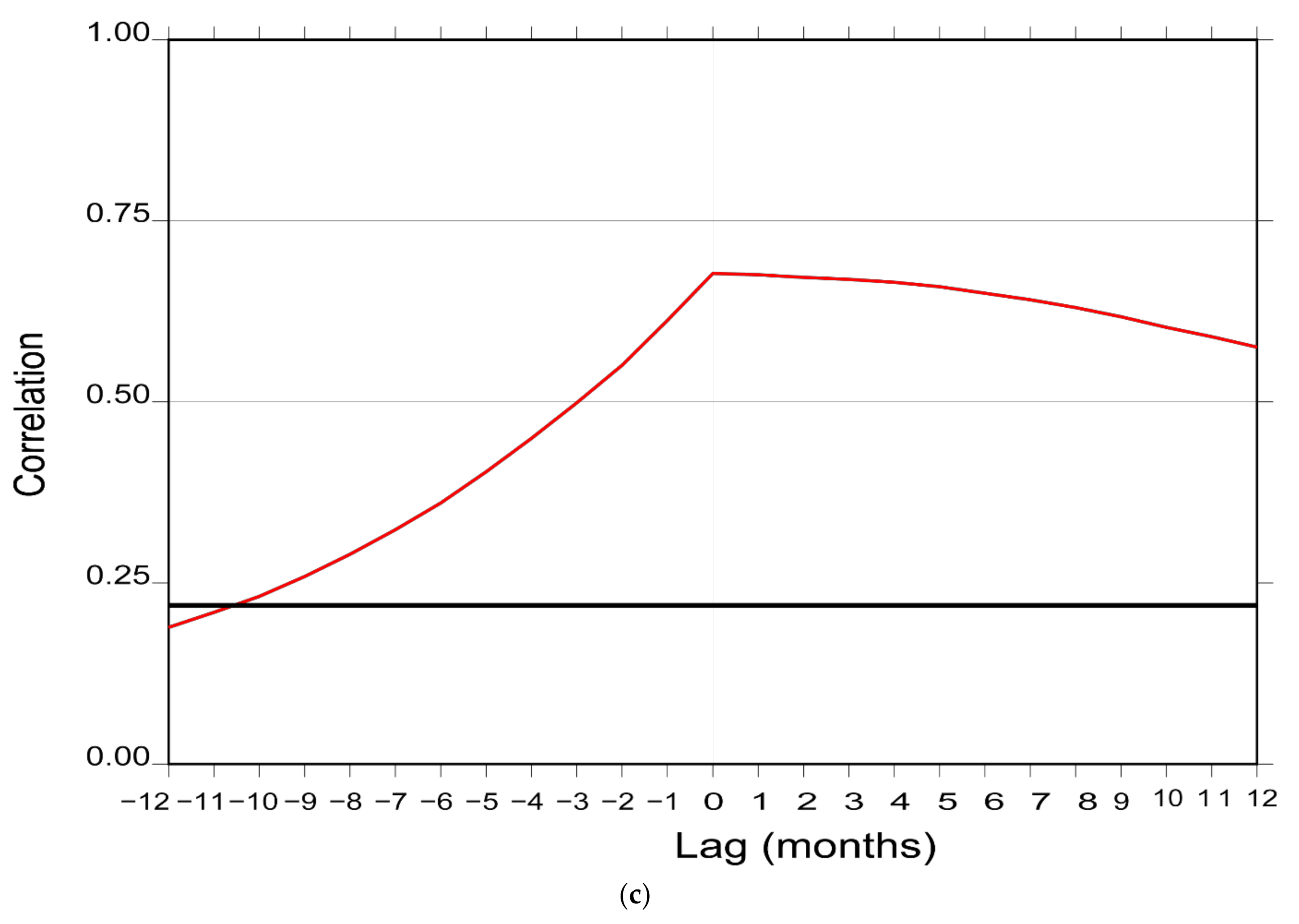
Figure 6.
Analysis of mass variation in western Himalaya. (a) Mode 1 of GRACE; (b) Mode 1 of Table 1 of SWE (c).
Figure 6.
Analysis of mass variation in western Himalaya. (a) Mode 1 of GRACE; (b) Mode 1 of Table 1 of SWE (c).
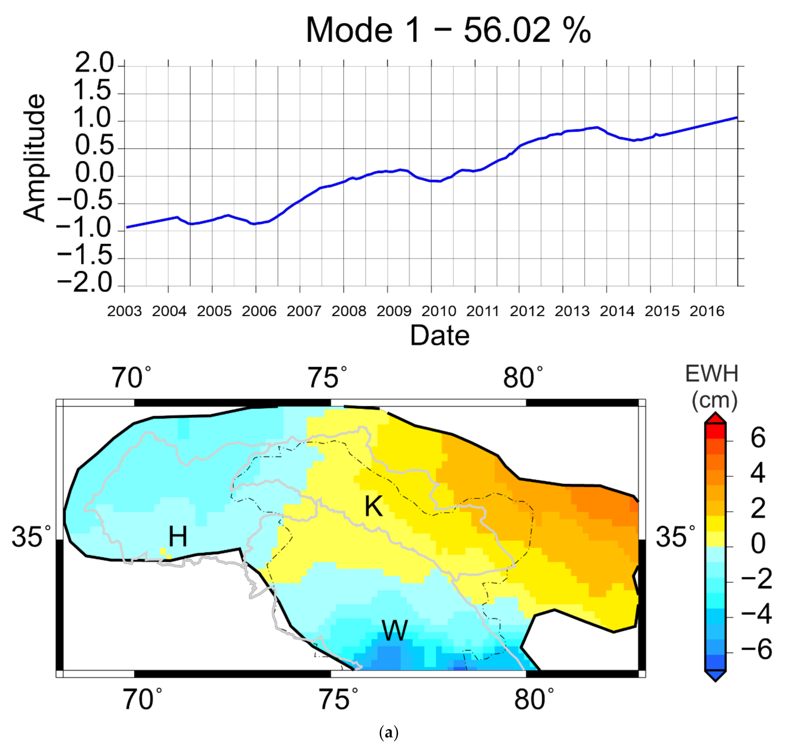

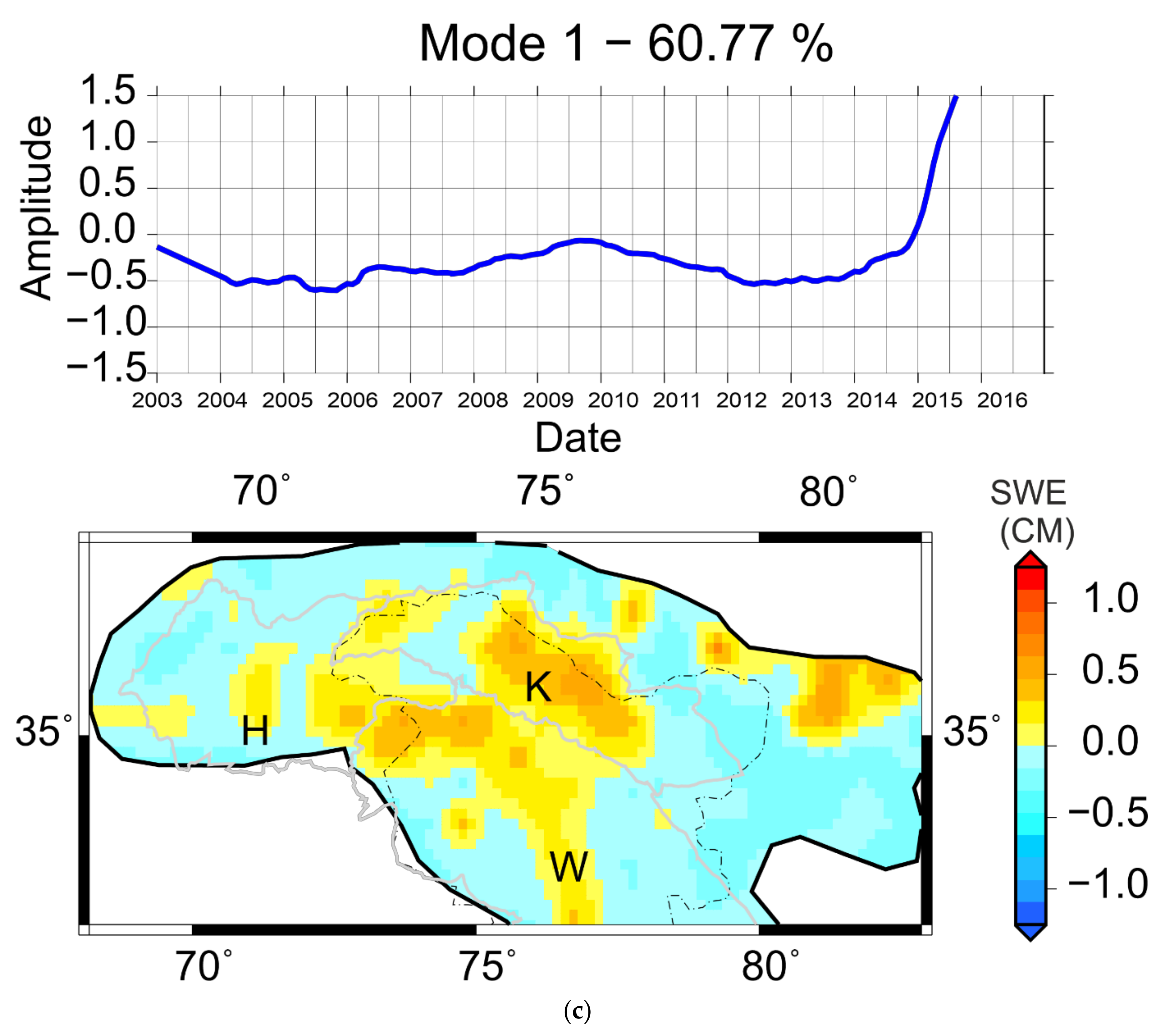
Figure 7.
Comparing GRACE with data with in situ observations. (a) Interannual Mode 1 with Glacier locations, Kulkarni et al. (2014) [20], marked in red and from Azam et al. (2016) [48] is in black circle. (b) Cumulative glacier mass balance from Kulakarni et al. (2014) and Azam and others (2016), versus GRACE interannual Mode 1 time series. Time series of Azam et al. (2016) is scaled to match other two time series, for ease of comparison.


Table 1.
Causal relationships of Himalaya Mode 1.
| F-Statistic | Snowfall | Critical Value | Rainfall | Critical Value |
|---|---|---|---|---|
| East | 5.93 | 17.48 | 183.74 | 17.48 |
| Central | 7.96 | 6.79 | 35.7275 | 17.48 |
| West | 12.86 | 5.49 | 8.85 | 17.48 |
Table 2.
Statistics of west Himalaya Mode 1 vs. climatic variables.
| Correlation | Lag | F-Statistic | Critical Value |
|---|---|---|---|
| 0.5 | 0 | 6.87 | 3.9 |
| 0.69 | 0 | 17.69 | 3.9 |
Publisher’s Note: MDPI stays neutral with regard to jurisdictional claims in published maps and institutional affiliations. |
© 2021 by the authors. Licensee MDPI, Basel, Switzerland. This article is an open access article distributed under the terms and conditions of the Creative Commons Attribution (CC BY) license (http://creativecommons.org/licenses/by/4.0/).
Share and Cite
MDPI and ACS Style
Munagapati, H.; Tiwari, V.M. Spatio-Temporal Patterns of Mass Changes in Himalayan Glaciated Region from EOF Analyses of GRACE Data. Remote Sens. 2021, 13, 265. https://doi.org/10.3390/rs13020265
AMA Style
Munagapati H, Tiwari VM. Spatio-Temporal Patterns of Mass Changes in Himalayan Glaciated Region from EOF Analyses of GRACE Data. Remote Sensing. 2021; 13(2):265. https://doi.org/10.3390/rs13020265
Chicago/Turabian StyleMunagapati, Harika, and Virendra M. Tiwari. 2021. "Spatio-Temporal Patterns of Mass Changes in Himalayan Glaciated Region from EOF Analyses of GRACE Data" Remote Sensing 13, no. 2: 265. https://doi.org/10.3390/rs13020265
Note that from the first issue of 2016, this journal uses article numbers instead of page numbers. See further details here.