Abstract
Despite its wide applications, the spatiotemporal fusion of coarse- and fine-resolution satellite images is limited primarily to the availability of clear-sky fine-resolution images, which are commonly scarce due to unfavorable weather, and such a limitation might cause errors in spatiotemporal fusion. Thus, the effective use of limited fine-resolution images, while critical, remains challenging. To address this issue, in this paper we propose a new phenological similarity strategy (PSS) to select the optimal combination of image pairs for a prediction date. The PSS considers the temporal proximity and phenological similarity between the base and prediction images and computes a weight for identifying the optimal combination of image pairs. Using the PSS, we further evaluate the influence of input data on the fusion accuracy by varying the number and temporal distribution of input images. The results show that the PSS (mean R = 0.827 and 0.760) outperforms the nearest date (mean R = 0.786 and 0.742) and highest correlation (mean R = 0.821 and 0.727) strategies in both the enhanced spatial and temporal adaptive reflectance fusion model (ESTARFM) and the linear mixing growth model (LMGM), respectively, for fusing Landsat 8 OLI and MODIS NDVI datasets. Furthermore, base images adequately covering different growth stages yield better predictability than simply increasing the number of base images.
1. Introduction
Satellite data with a high spatiotemporal resolution are highly desired for studying ecological processes and impacts in heterogeneous landscapes. However, a single satellite sensor provides data with either a high temporal frequency or a high spatial resolution due to the trade-offs among the spatial, temporal, and spectral resolutions [1]. For example, the Moderate Resolution Imaging Spectroradiometer (MODIS) has a frequent revisit cycle but a coarse resolution ranging from 250 m to 1 km, whereas Landsat satellite data have a finer spatial resolution of 30 m but a restricted temporal resolution [1]. To exceed the physical limitations of individual satellite data, a feasible solution has been to spatiotemporally fuse frequent coarse-resolution images (hereafter referred to as coarse images) with less frequent fine-resolution images (hereafter referred to as fine images) [2,3,4]. Accordingly, many fusion algorithms have been developed; the most representative examples include weight function-based [3,5,6,7,8,9], unmixing-based [10,11,12,13], Bayesian-based [14], and learning-based [15,16,17] algorithms, as well as hybrid methods that combine two or more of the aforementioned techniques [2,8,9,18,19]. A detailed review can be found in [4].
All of these spatiotemporal fusion methods use the spatial information from fine images and the temporal information from coarse images to predict a fine image at an unobserved date. Thus, spatiotemporal fusion methods require at least one pair of images (one coarse and one fine), which serve as the basis for prediction and were referred to as base images. Previous studies have recognized that the performance of a spatiotemporal fusion algorithm depends strongly on the base image pair quality [20,21]. Hence, to improve the spatiotemporal data fusion accuracy, efforts have been made to evaluate the influence of input image pairs [7,21] and optimize the strategy for selecting base data [20,21].
Researchers have discovered that the spatiotemporal data fusion accuracy depends on the similarity between the base and prediction images [1,7,19,21]. Since the land surface is always changing, the fusion accuracy declines as the base-prediction time interval increases [21,22]. Thus, the nearest data strategy (NDS), which selects the image pair temporally nearest to the prediction data, is widely used, such as in the enhanced spatial and temporal adaptive reflectance fusion model (ESTARFM) [1] and the flexible spatiotemporal data fusion (FSDAF) model [19]. Based on the same similarity criterion, Wang et al. [7] proposed choosing between the NDS and the highest correlation strategy (HCS) in an operational data fusion framework. The HCS selects the image pair featuring the highest correlation with the coarse image at the prediction date. A comparative study found that the HCS performs better than the NDS in the STARFM [21]. The accuracy of spatiotemporal fusion also depends on the consistency between the radiometric characteristics and geometries of the coarse and fine images [7,21]. As such, a recent study proposed a cross-fusion method that combines similarity and consistency criteria; however, this method is very complicated and can handle only cases involving five input image pairs [20]. As a result of the difficulties in base data selection, Liu et al. [23] suggested using multiple base image pairs to generate several prediction images on the same date and combining these images to produce a final prediction image through a weighted sum.
Nonetheless, despite the small number of strategies developed for base data selection, major problems have been confronted in cases with very limited input data. First, it is very difficult to acquire two clear-sky fine images in a reasonable temporal proximity due to unfavorable weather and long revisit periods. For instance, Landsat images are acquired at a 16-day interval [3], and the annual mean global cloud cover was derived as about 35% from the Landsat ETM+ scenes acquired one or more times in each year [24]. Moreover, in most cases, clear-sky fine images are scarce during periods of rapid vegetation growth due to frequent rains. Second, the existing strategies for the selection of base data do not consider the seasonal similarity and symmetry of the land surface. Previous studies noted the important role that seasonal similarity plays in the spatiotemporal data fusion performance; for example, image pairs from different seasons resulted in the poorest predictions [7], while those from the same season (i.e., growing or nongrowing season) yielded better predictions [21]. Nevertheless, the NDS, which is a highly common algorithm, considers only the impacts of the base-prediction time interval and neglects the influence of seasonal variation on image similarity. In contrast, the HCS relies on the correlations between base-prediction coarse images, and these correlations might be inconsistent with those between base-prediction fine images due to the scale effect [25,26,27]. Third, few studies have evaluated the impacts of the number and timing of input image pairs on time-series predictions using a specific strategy. Gevaert and García-Haro found that the STARFM gives poor time-series predictions with one or two image pairs but performs well with six image pairs using the NDS [2]. Nevertheless, to date, the conditions under which input image pairs can result in reliable time-series predictions have yet to be ascertained.
To address these issues, we aimed to optimize the base data selection strategy for spatiotemporal fusion and identify the optimal number and timing of input image pairs in time-series predictions for landscapes with seasonal variations. Specifically, we propose a new automatic similarity-based strategy, namely, the phenological similarity strategy (PSS), to quantify the phenological similarity, seasonal symmetry, and temporal proximity and then compute weights for identifying the optimal combination of image pairs. The performance of the PSS is also compared with that of the NDS and HCS in spatiotemporal fusion algorithms. Using the PSS, this paper further investigates the influences of the number and timing of input image pairs on year-round predictions.
To implement the above strategies, this paper chose two typical spatiotemporal data fusion algorithms to test the performance of each fusion strategy: the weight function-based ESTARFM [6] and the unmixing-based linear mixing growth model (LMGM) [28]. Both algorithms were applied in the context of blending Landsat 8 Operational Land Imager (OLI) and MODIS normalized difference vegetation index (NDVI) data to synthesize a new NDVI dataset with a high spatiotemporal resolution. We choose to blend NDVI data instead of reflectance data because of the following reasons:
- (1)
- There is a direct demand for high-spatiotemporal resolution NDVI products in various environmental applications, such as modeling evapotranspiration and net primary production [29,30], and thus, there is an increasing interest in the spatiotemporal fusion of NDVI [22,23,28,31].
- (2)
- Directly fusing NDVI is more accurate and efficient than fusing multiband reflectance data and subsequently computing vegetation indices (VIs) because there is less error propagation [32,33,34].
- (3)
- Fused NDVI products can characterize the vegetation phenology.
- (4)
- The results derived from this approach provide a reference for fusing multiband reflectances or other land surface parameters.
2. Materials and Methods
2.1. Study Site and Data
The study area is located in the Guanzhong region of Shaanxi Province, China, within 110°15′–100°26′ E, 35°26′–35°34′ N (Figure 1). The Guanzhong region features complex topography, with the southern edge of the Loess Plateau to the north and the steep northern slope of the Qinling Mountains to the south. Coupled with the special climatic conditions and the high concentration of population and industry, this region typically exhibits frequent clouds, fog, and haze. As shown in Table 1, the number of clear (cloud coverage < 5%) Landsat 8 OLI images during 2013–2019 in the Guanzhong region is very low. For scene 128/037, there are fewer than two clear Landsat 8 OLI images in an entire year. Hence, the study area is located in scene 126/035 (highlighted in bold texts in Table 1), which generally has more clear images than the other scenes and covers an area of 18 × 18 km2.

Figure 1.
Map of the study area. (a) Visible-near-infrared composite Landsat 8 Operational Land Imager (OLI) image on 24 August 2014. (b) Land cover classification from Moderate Resolution Imaging Spectroradiometer (MODIS) normalized difference vegetation index (NDVI) time-series data in 2014.

Table 1.
Numbers of cloud-free Landsat 8 OLI images during 2013–2019 over the Guanzhong region.
Since the Landsat 5 Thematic Mapper (TM) was decommissioned on 5 June, 2013 [35] and since the Landsat 7 Enhanced TM Plus (ETM+) sensor encountered the permanent failure of its scan line corrector (SLC) on 31 May, 2003 [36], only Landsat 8 OLI images provide high-quality spatially continuous 30-m resolution images after 2013; hence, Landsat 8 OLI images were used in the study. As shown in Table 1, eight clear Landsat 8 OLI images are available for 2014. Their acquisition dates are 12 January, 28 January, 4 May, 20 May, 24 August, 12 November, 28 November, and 30 December, 2014, which correspond to MODIS DOY 1, 17, 129, 145, 225, 305, 321, and 353, respectively. All Landsat 8 OLI surface reflectance and NDVI images were downloaded from the Earth Resources Observation and Science (EROS) Science Processing Architecture (ESPA, https://espa.cr.usgs.gov/) on-demand interface as processed products [37] from Landsat collection 1 in the UTM/WGS-84 projection system. Figure 2 compares the downloaded Landsat surface reflectance and NDVI values on 24 August 2014. The surface reflectance values from the red and near-infrared (NIR) bands are concentrated mainly within 0.02~0.1 and 0.2~0.4, respectively; thus, the resulting NDVI values are concentrated within 0.6~0.9. In addition, the corresponding MOD13Q1 NDVI products at a 16-day interval and 240-m resolution for all of 2014 were downloaded and converted into the UTM/WGS-84 projection system. These MODIS NDVI time-series data were used to classify the study area into four different land cover classes through the K-means clustering algorithm as dense forest (16.44%), moderate forest (50.81%), cropland (24.76%), and nonvegetation (7.98%), as shown in Figure 1b. The eight downloaded Landsat 8 OLI NDVI products and the corresponding MODIS NDVI products were used as input image pairs for spatiotemporal fusion.
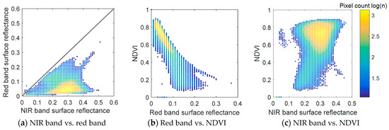
Figure 2.
Comparisons among the Landsat 8 OLI red band and NIR band surface reflectances and NDVI within the study area on 24 August 2014.
2.2. Fusion Algorithms Tested
Two spatiotemporal fusion algorithms were evaluated: the weight function-based ESTARFM [6] and the unmixing-based LMGM [28]. These two algorithms were selected due to their (i) minimum input requirements, (ii) software availability, (iii) ability to handle both homogeneous and heterogeneous landscapes, and (iv) wide acceptance within the remote sensing community.
The ESTARFM is a particular improvement over the classic STARFM [3] for more complex situations. The ESTARFM assumes a single rate of change over the entire period between the two input Landsat acquisitions [1,6] and resolves this rate of change by linearly regressing the reflectance changes in fine-resolution pixels and the coarse-resolution pixels of the same endmember. The ESTARFM thus requires a minimum of two Landsat-MODIS image pairs and an additional MODIS image on the prediction date.
In contrast, the LMGM algorithm [28] assumes a linear rate of change in the NDVI during a short period and unmixes the NDVI growth rates from coarse-resolution pixels to fine-resolution pixels. As a result that the assumption of linear NDVI change is reasonable during a short period, the LMGM predicts long-term NDVI variations by combining several short-term predictions using Equation (1),
where tm is the acquisition date of the base Landsat image, tm + 1 and tm + 2 are the two prediction dates (tm < tm + 1 < tm + 2), Lm and Lm + 2 are the Landsat NDVI values at tm and tm + 2, and km + 1 and km + 2 are the NDVI growth rates at the Landsat scale from tm to tm + 1 and from tm + 1 to tm + 2, respectively. Therefore, the LMGM requires one base image pair and all MODIS images on the interval dates from the base date to the prediction date, unlike the ESTARFM, which requires only one additional MODIS image on the prediction date. For two or more base image pairs, the LMGM algorithm can combine the images on the same prediction date fused by different image pairs through a time-weighted sum.
For a more detailed description of the ESTARFM and LMGM algorithms, please refer to [6,28], respectively.
2.3. Phenological Similarity Strategy (PSS) for Base Data Selection
We propose a new strategy, i.e., the PSS, to integrate the impacts of phenological similarity and temporal proximity into the selection of base data. The PSS uses a weighting procedure to compute the final weights, namely, the PSS weights, to identify the optimal combination of image pairs for the prediction date. The PSS weights are derived through three major steps.
In step 1, the PSS divides an entire year into different phenological periods based on the MODIS NDVI time-series data. Figure 3 shows the mean MODIS NDVI growth curves corresponding to each land cover type. The first-order differentials in the MODIS NDVI growth curves in Figure 3b represent the NDVI growth rates; these curves were used to identify the critical transitional dates. The four periods are divided as follows: (1) a pregrowth period that ends at the maximum positive growth rate, (2) a rapid growth period that ends as the growth rate decreases to zero, (3) a peak and rapid senescence period that ends at the minimum negative growth rate, and (4) a postgrowth period with typically low NDVI values. Cropland exhibits double-season growth curves, for which the above phenological division is still valid. For double-season cropland, periods (2) and (3) represent the first and second growing seasons, respectively. Furthermore, despite the complexity and mixture of land cover types in the study area, stages 1 and 4 represent stable temporal curves with subtle changes, while stages 2 and 3 exhibit rapid change profiles.
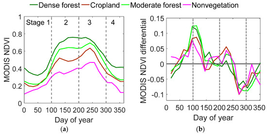
Figure 3.
Schematic diagram of the phenological stage division process. (a) MODIS NDVI time curves and (b) the first-order differentials in the MODIS NDVI for the typical land cover classes in 2014 in the study area.
Based on the division of phenological stages, the PSS further assigns a phenological similarity weight for each pair of base-prediction dates, as shown in Table 2. Generally, the base date in the same stage as the predication date has the highest weight of 1.0. Otherwise, such a weight is determined based on the seasonal symmetry and temporal proximity. In particular, stage 1 is most similar to stage 4, followed by stages 2 and 3, corresponding to weight values of 0.75, 0.5, and 0.25, respectively. Stage 2 is most similar to stage 3, followed by stages 1 and 4.
Table 2.
Phenological similarity weights between the base and prediction dates.
In step 2, the PSS calculates two types of temporal proximity, the absolute temporal proximity and mirror temporal proximity between the prediction and base dates (tp and tb, respectively), the minimum of which is normalized to 0~1 as the weight for the temporal proximity. The absolute temporal proximity is calculated as the absolute distance of tb from tp. Assuming that the vegetation phenological curve is symmetrical, we can transfer tb to a symmetrical point (date) on the curve by subtracting tb from the total length (days) of a year (T), which we will refer to as the mirror date. Then, the mirror temporal proximity is calculated as the distance of this mirror date (T − tb) from tp. The minimum temporal proximity is calculated as:
where T = 365 for nonleap years. Using two types of temporal proximity, PSS quantifies a similarity-based temporal proximity between two dates. For example, if tp is DOY 353 and tb is DOY 1, the absolute temporal proximity between tp and tb is 352, while the similarity-based temporal proximity is |tp − (365 − tb)| = 11. The latter better represents the relatively high similarity between images on tp and tb than the former.
In step 3, the PSS combines the weights for phenological similarity () and temporal proximity () to derive a final weight, namely, the PSS weight, using the following:
Combining the two weights is necessary to prioritize the use of the image pair from the same season as the prediction date. For example, if tp is DOY 353, the tb values on DOY 1 and 364 have the same values of , while combining with helps identify the image on DOY 364 as the more appropriate image pair.
For the prediction date tp, the base date that derives the highest PSS weight is regarded as the most appropriate image pair. For fusion algorithms that require a minimum of two base image pairs, such as the ESTARFM algorithm, a combined weight for the two base dates t1 and t2 is calculated as a weighted sum of the weights for t1 and t2 as follows:
where the base date with a higher weight plays a more important role than that with a lower weight. The PSS weight for two dates ranges from 0 to 1.5.
For algorithms that can work with both one and two base image pairs (e.g., the LMGM algorithm), the PSS weight for one base image pair can be multiplied by a scaling factor of 1.5 to be comparable to the PSS weight for two base image pairs.
2.4. Applying Fusion Algorithms
Both the ESTARFM and the LMGM were applied by predicting a Landsat NDVI image on some date using all possible combinations of base image pairs. We divided the eight Landsat NDVI images from 2014 into seven training images (Nin-all = 7) and one independent validation image on DOY 145. All possible combinations of base image pairs were selected from the Nin-all training image pairs and the remaining Landsat NDVI images (including the image on DOY 145) were used to evaluate the accuracy of the simulation image. The Landsat NDVI image on DOY 145 was not included in the base data selection so that the validation included at least one actual Landsat image at the rapid vegetation growth stage for all possible combinations of base image pairs.
The ESTARFM requires a minimum of two base image pairs (i.e., Nmin = 2) and thus was executed times, generating a total of 126 fused images. For the LMGM, this study considered only the cases involving one or two base image pairs, i.e., Nmin = 1 and 2. This is reasonable because a third or more additional base image pairs will have much less impact on the prediction image due to their lower time weights in combining multiple prediction images. Thus, the LMGM was executed times, generating a total of 175 fused images.
When implementing the fusion algorithms, the default NDVI threshold-based classification was used for both the ESTARFM and the LMGM algorithms. The other required parameters, such as the search window size and the minimum number of similar pixels in the ESTARFM, were all kept as the default values.
All the fused images were evaluated against actual Landsat NDVI images using two major statistical indicators, namely, the correlation coefficient (R) and root mean squared error (RMSE). R was used to evaluate the linear relationship between the predicted and actual images, while RMSE was used to gauge the prediction errors. Both metrics are widely used to evaluate the performance of spatiotemporal data fusion algorithms [1,4,6,19,21].
2.5. Applying Fusion Strategies
Three base data selection strategies were evaluated: the NDS, HCS, and PSS. All three strategies were applied to select Nmin base image pairs from the Nin input image pairs, where Nin > Nmin. Here we constrain Nin = 3, 4, and 5 to represent cases of limited input data. For each value of Nin, the Nin input image pairs were randomly selected from the Nin-all training image pairs until all possible combinations of Nin input image pairs were included.
Among the Nin input image pairs, the PSS computed the PSS weights for all candidate image pairs, the number of which was for the ESTARFM and for the LMGM. The Nmin image pairs with the highest PSS weights were identified as the optimal combination of image pairs, where Nmin is 2 for the ESTARFM and Nmin can be either 1 or 2 for the LMGM (in other words, the PSS can automatically determine whether to use one or two image pairs in the LMGM). The NDS evaluated the absolute temporal proximities between each prediction date and all candidate base dates, and the Nmin image pairs nearest to the prediction date were identified as the optimal combination of image pairs. The HCS analyzed the R values between the MODIS NDVI images at the prediction date and all candidate base dates. Then, the Nmin image pairs featuring the highest correlation with the MODIS NDVI image on the prediction date were selected as the optimal combination of image pairs. The general processes of the NDS and HCS were the same for the ESTARFM. However, for the LMGM, neither the NDS nor the HCS could automatically determine whether to use one or two image pairs. Thus, both the NDS and HCS were implemented for two cases: one case involved the selection of one optimal image pair (i.e., referred to as LMGM-NDS-1 and LMGM-HCS-1, respectively), and the other involved the selection of the optimal combination of two image pairs (i.e., referred to as LMGM-NDS-2 and LMGM-HCS-2, respectively).
As described in Section 2.4, the images fused by all possible combinations of Nmin image pairs were generated using both the ESTARFM and the LMGM. Thus, the fusion algorithms were not explained again here. We directly extracted the images fused by the optimal combination of image pairs; for each combination of Nin input image pairs, a total of (8-Nin) fused images were extracted and evaluated.
2.6. Quantifying the Temporal Distribution of Input Image Pairs
The PSS was also used to quantify the temporal distribution of Nin input image pairs. According to the phenological division described in Section 2.3, we assigned a code for each date among the Nin input Landsat acquisitions. We then sorted the Nin date codes in ascending order and combined the codes to compute a final code using , where ci represents the ith date code amongst the Nin date codes. This final code describes the distribution of Nin input image pairs across four different phenological stages; we refer to this final code as the distribution code.
Among the possible combinations of the Nin input image pairs, some combinations might share the same distribution code, e.g., for input DOY 1, 225, and 321 and input DOY 16, 225, and 353. The images fused by input image pairs with the same distribution code were grouped to compute the mean and standard deviation (STD) for the corresponding R and RMSE values. We further analyzed the relationship between the distribution code and the fusion accuracy to help identify under which conditions the fusion algorithms using the PSS produce satisfactory time-series predictions with limited input data.
3. Results
3.1. Validity of the Phenological Similarity Strategy (PSS)
3.1.1. Time Interval vs. Fusion Accuracy
We analyzed the relationship between the ESTARFM fusion accuracy and the base-prediction time interval, as shown in Figure 4. The maximum and minimum time intervals between the prediction date and two base dates were computed and presented on the x-axis and y-axis, respectively. Generally, three cases result in high accuracy with R ≥ 0.7, including (1) a small minimum time interval (i.e., <96), (2) a small maximum time interval (i.e., <120), and (3) a large maximum time interval (i.e., >320). A minimum time interval > 96 and a maximum time interval <320 result in the lowest accuracy (R < 0.7; RMSE > 0.2) for the fused images, indicating a nonlinear relationship between the time interval and the performance of the ESTARFM. In particular, when the maximum and minimum intervals are both large (i.e., >300), the fusion accuracy is still high with R ≥ 0.8 and RMSE ≤ 0.2. This finding is explainable using the PSS because the base image pairs, although distant from the prediction date, could be phenologically similar to the prediction image. However, the NDS cannot consider such similarity and may not identify the optimal combination of base image pairs correctly, thereby increasing the uncertainty in spatiotemporal data fusion.
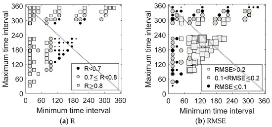
Figure 4.
Relationships between the fusion accuracies of the enhanced spatial and temporal adaptive reflectance fusion model (ESTARFM) and the time interval between the base and prediction dates.
Figure 5 presents a nonlinear relationship between the fusion accuracy of the LMGM with one base image pair and the base-prediction time interval. The fusion accuracy decreases rapidly as the base-prediction time interval increases from 0 to 180, reaches its minimum at time intervals between 180 and 240, and increases gradually as the time interval increases from 240 to 365. Such nonlinear changes also confirm that the NDS may not be feasible in some cases.
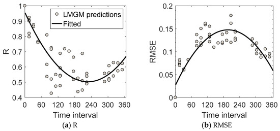
Figure 5.
Relationships between the fusion accuracies of the linear mixing growth model (LMGM) with one base image pair and the time interval between the base and prediction dates.
Furthermore, Figure 6 reveals a complex relationship between the fusion accuracy of the LMGM with two base image pairs and the base-prediction time interval. Two cases, namely, (1) with a small minimum interval (i.e., <48) and a small maximum interval (i.e., <60) and (2) with a small minimum interval (i.e., <48) and a large maximum interval (i.e., >288), result in the highest accuracy with R ≥ 0.7 and RMSE ≤ 0.1. In contrast, when the minimum interval is <60, the fusion accuracy decreases first as the maximum interval increases and then slightly increases when the maximum interval is >240. When the minimum interval is >60, the fusion accuracy decreases as the maximum interval increases. Such changes in the fusion accuracy with the base-prediction interval are different from those of the ESTARFM algorithm. As a result that the LMGM combines short-term predictions to derive a long-term prediction, errors will propagate in this sequential fusion process, thereby decreasing the fusion accuracy as the time interval increases.
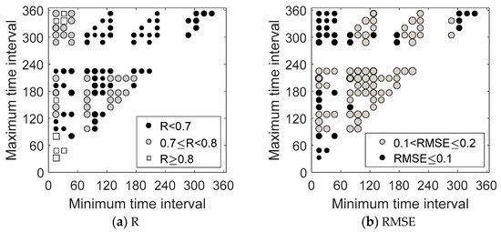
Figure 6.
Relationships between the fusion accuracies of the LMGM with two base image pairs and time interval between the base and prediction dates.
3.1.2. MODIS Correlation vs. Fusion Accuracy
We also analyzed the relationship between the ESTARFM accuracy and the correlations between the MODIS NDVI images (hereafter referred to as the MODIS correlation), as shown in Figure 7. A weighted sum of the correlation coefficients (r) was calculated for two pairs of base and prediction images using , where t1 and t2 are two base dates and tp is the predication date. The weighted sum of the MODIS correlations has a good linear relationship with (but is not indicative of) the ESTARFM fusion accuracy. R values from 0.25 to 0.85 correspond to the weighted sum of MODIS correlations from 0.8 to 1.2. In other words, only very high values of the weighted sum of MODIS correlations (i.e., >1.2) result in high accuracy with R > 0.8. Moreover, when the weighted sum of MODIS correlations is <1.2, it is very difficult to identify the optimal combination of base image pairs.
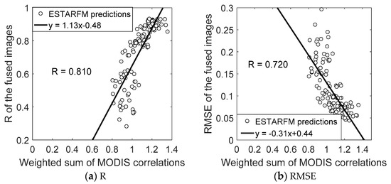
Figure 7.
Relationships between the fusion accuracies of the ESTARFM and the weighted sum of correlations for two pairs of base-prediction MODIS NDVI images.
Figure 8 presents a linear relationship between the LMGM accuracy and sum of MODIS correlations. Similar to the ESTARFM, the weighted sum of MODIS correlations can hardly distinguish the image pairs that have better predictability. For example, even when the weighted sum of MODIS correlations is high (>1.2), the R values of the prediction images on DOY 17 vary from 0.48 to 0.90 (mean R = 0.59). This reinforces the expectation that the MODIS correlations are not a good indicator of the spatiotemporal fusion accuracy.
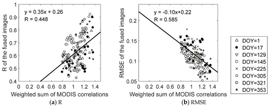
Figure 8.
Relationships between the fusion accuracies of the LMGM and weighted sum of correlations for two pairs of base and prediction MODIS NDVI images.
3.1.3. PSS Weight vs. Image Similarity
To further test the validity of the PSS, we used R as an indicator of image similarity and evaluated the relationship between the PSS weight and the similarity of actual images at the MODIS and Landsat resolutions, as shown in Figure 9. A strong linear relationship between the PSS weight and image similarity is observed for both the actual MODIS and the Landsat NDVI images, and the linear correlation between the PSS weight and the Landsat image similarity (R = 0.925) is much higher than that between the PSS weight and the MODIS image similarity (R = 0.591). This finding reinforces that the PSS can accurately represent the similarity between actual fine images and will be useful for base data selection in spatiotemporal data fusion.
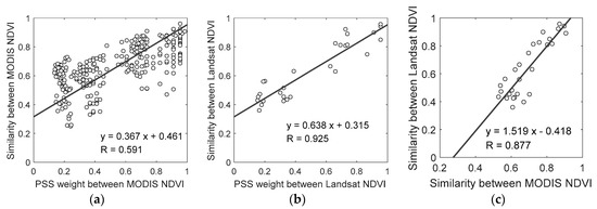
Figure 9.
Scatterplots of the phenological similarity strategy (PSS) weights and similarities calculated for actual (a) MODIS NDVI images and (b) Landsat NDVI images and (c) scatterplot between the MODIS NDVI image similarity and Landsat NDVI image similarity.
For comparison, we also analyzed the relationship between the MODIS image similarity and the Landsat image similarity, as shown in Figure 9c. Although linearly related to the Landsat image similarity, the MODIS image similarity has a narrower range (0.55~1.0 vs. 0.2~1.0) and a lower correlation coefficient (R = 0.877 vs. R = 0.925) than the PSS weight does. This indicates that the PSS weight has a better linear correlation with the Landsat image similarity.
3.1.4. PSS Weight vs. Fusion Accuracy
We further analyzed the relationship between the PSS weight and the ESTARFM fusion accuracy, as shown in Figure 10. The ESTARFM fusion accuracy increases very rapidly as the PSS weight increases from 0 to 0.6 and then increases slightly as the PSS weight continues to increase, representing a nonlinear relationship with the PSS weight. When the PSS weight is ≥0.6, the ESTARFM fusion accuracy reaches and stays at a high level (R > 0.8 and RMSE < 0.08). Hence, a continual increase in the PSS weight will lead to continual increases in the fusion accuracy. In general, a higher PSS weight is more likely to produce a higher accuracy.
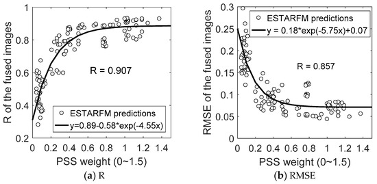
Figure 10.
Scatterplots of the fusion accuracies and PSS weights for all ESTARFM predictions with two base image pairs.
Likewise, Figure 11 shows the relationship between the LMGM fusion accuracy and the PSS weight. In general, the fusion accuracy (R) linearly increases as the PSS weight increases. Some data points deviate from the trend line, probably because each prediction date has a specific trend. In comparison to the MODIS correlations presented in Figure 9, the PSS weight has a wider range from 0 to 1.5. For the prediction images on DOY 17, a high PSS weight (i.e., >1.2) results in a high fusion accuracy with R > 0.7. In general, a high PSS weight is indicative of a high fusion accuracy.
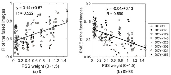
Figure 11.
Scatterplots of the fusion accuracies and PSS weights for all LMGM predictions with one and two base image pairs.
3.2. Comparison of Different Strategies for Base Data Selection
Figure 12 compares the fusion accuracies of different strategies in the ESTARFM algorithm. There are a total of 392 data points, each of which represents the accuracy of an image fused by applying the NDS, HCS, and PSS to the same combination of input image pairs. Generally, the predictability of the image pairs selected by the three strategies are as follows: PSS (mean R = 0.827 and mean RMSE = 0.088) > HCS (mean R = 0.821 and mean RMSE = 0.089) > NDS (mean R = 0.786 and RMSE = 0.100). On the scatterplots provided in Figure 12, the data points on the 1:1 line indicate that the two strategies select the same combination of base image pairs and achieve identical accuracy. Figure 12a reveals that the NDS and PSS selected different image pairs among 153 data points and the accuracy of the PSS (mean R = 0.875 and mean RMSE = 0.068) is significantly higher than that of the NDS (mean R = 0.771 and mean RMSE = 0.098). As in Figure 12b, the HCS and PSS selected different image pairs among 169 data points; again, the accuracy of the PSS (mean R = 0.799 and mean RMSE = 0.098) is higher than that of the HCS (mean R = 0.788 and mean RMSE = 0.101). This indicates that using the PSS in the ESTARFM algorithm can achieve higher accuracy than using the NDS or HCS.
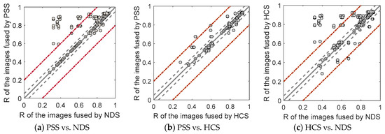
Figure 12.
Comparison of fusion accuracies using the nearest data strategy (NDS), highest correlation strategy (HCS), and PSS in the ESTARFM algorithm. Gray solid lines represent the 1:1 line, gray dashed lines represent ±0.05 of the 1:1 line, and red dashed lines represent ±0.2 of the 1:1 line.
Figure 13 compares the accuracies of using one image pair and two image pairs using the NDS and HCS in the LMGM algorithm. In general, the average fusion accuracies of the four strategies are LMGM-NDS-1 (R = 0.742) > LMGM-HCS-1 (R = 0.727) > LMGM-HCS-2 (R = 0.709) > LMGM-NDS-2 (R = 0.674). This order indicates that using one image pair has better predictability than using two image pairs for both the NDS and the HCS in the LMGM algorithm. In the cases involving one base image pair, the NDS features better predictability than the HCS, while in the cases involving two base image pairs, the HCS exhibits better predictability than the NDS.
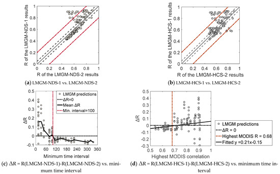
Figure 13.
Comparison of the LMGM accuracy using one and two image pairs with the NDS and HCS strategies. In (a,b), gray solid lines represent the 1:1 line; gray dashed lines represent ±0.05 of the 1:1 line; and the red dashed lines represent ±0.2 of the 1:1 line.
We further analyzed the reason for the better performance of using one image pair than of using two image pairs for both the NDS and the HCS. Figure 13c shows the relationship of the R difference between LMGM-NDS-1 and LMGM-NDS-2 with the minimum base-prediction time interval. A small minimum base-prediction time interval (i.e., <100) evidently leads to the better performance of LMGM-NDS-1, while a large minimum base-prediction time interval (i.e., >100) results in the better performance of LMGM-NDS-2. This finding indicates that one image pair that is adequately near the prediction date is sufficient to achieve a high accuracy. For two image pairs distant from the prediction date, using both might enhance the fusion accuracy due to the provision of complementary information and error compensation.
Figure 13d shows the relationship of the R difference between LMGM-HCS-1 and LMGM-HCS-2 with the highest base-prediction MODIS correlation. When the highest base-prediction MODIS correlation is <0.68, LMGM-HCS-2 has better predictability. When the highest MODIS correlation is ≥0.68, LMGM-HCS-1 has slightly better predictability than LMGM-HCS-2 on average, but in some cases, LMGM-HCS-2 is still better than LMGM-HCS-1. This again indicates that the MODIS correlation is not a very effective indicator for base data selection in the LMGM algorithm.
Figure 14 compares the accuracies of fused images using the PSS, NDS, and HCS in the LMGM algorithm. For all 518 data points, the accuracy of the fused images decreases in the following order: LMGM-PSS (mean R = 0.760 and mean RMSE = 0.096) > LMGM-NDS-1 (mean R = 0.742 and mean RMSE = 0.101) > LMGM-HCS-1 (mean R = 0.727 and mean RMSE =0.098) > LMGM-HCS-2 (mean R = 0.709 and mean RMSE = 0.099) > LMGM-NDS-2 (mean R = 0.674 and mean RMSE = 0.109). In general, LMGM-PSS produces a systematically higher accuracy than LMGM-NDS-1, LMGM-NDS-2, LMGM-HCS-1, and LMGM-HCS-2. This indicates that LMGM-PSS could combine the complementary strength of using one and two image pairs and is a valid tool for base data selection.
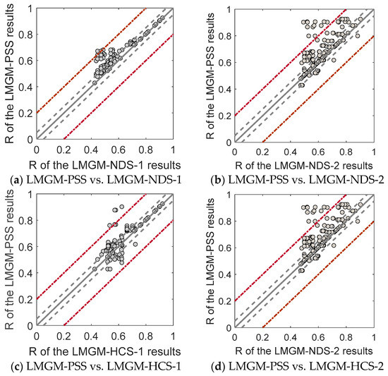
Figure 14.
Comparison of the fusion accuracies using the LMGM-PSS, LMGM-NDS-1, LMGM-NDS-2, LMGM-HCS-1, LMGM-HCS-2. Gray solid lines represent the 1:1 line. Gray dashed lines represent ±0.05 of the 1:1 line, and red dashed lines represent ±0.2 of the 1:1 line.
3.3. Influence of Input Data on the Fusion Accuracy
Using the phenological divisions obtained from the PSS, we analyzed the influences of the number and temporal distribution of input data on the fusion accuracy. Figure 15 presents the R and RMSE statistics of the images fused by the ESTARFM PSS using different combinations of base data (i.e., represented as the distribution codes and the number of input image pairs Nin). For Nin = 2, the base data coded as ‘23’, ’14’, ‘44’, and ‘11’ result in low accuracies (mean R < 0.70 and mean RMSE > 0.10), while the base data coded as ‘24’, ‘34’, ‘12’, ‘13’ result in stable, high accuracies (mean R > 0.80 and mean RMSE < 0.10). These results indicate that even with very limited data (Nin = 2), the ESTARFM could be highly accurate in year-round predictions given appropriate base image pairs. For Nin > 2, the base data with codes consisting only of digits ‘1’ and ‘4’, i.e., ‘144’, ‘114’, ‘144’, ‘1444’, ‘1144’, and ‘11444’, result in low accuracies (mean R < 0.7 and mean RMSE > 0.12), while all other combinations of base data result in very high accuracies with small deviations (mean R > 0.8 with STD < 0.10). This is understandable because the input image pairs at stages 1 or 4 are very similar and can hardly capture the spatial patterns for stages 2 and 3. Generally, the base data adequately covering all four stages generate highly accurate year-round predictions using the ESTARFM algorithm, indicating that an appropriate temporal distribution is more important than simply increasing the number of base image pairs. For example, adding one image pair at stages 2 or 3 to the base data coded ‘144’ increases the prediction accuracy significantly from R = 0.66 to R = 0.86 (new code = ‘1244’) or 0.87 (new code = ‘1344’). In contrast, adding one image pair at stages 1 or 4 to the base data ‘144’ reduces the accuracy from R = 0.66 to R = 0.65 (new code = ‘1144’) or R = 0.64 (new code = ‘1444’).
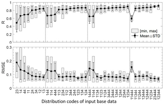
Figure 15.
R and RMSE statistics of the images fused by the ESTARFM PSS using different combinations of input base data.
Figure 16 presents the R and RMSE statistics of the images fused by the LMGM-PSS using different combinations of base data. The accuracies of the LMGM are generally lower than those of the ESTARFM. For Nin = 2, the base data coded as ‘23’, ‘11’, ‘13’, ‘44’, ‘12’, and ‘34’ result in relatively low accuracies (mean R < 0.70 and mean RMSE > 0.10), while the base data coded as ‘24’ and ‘14’ derive higher fusion accuracies (mean R > 0.70 and mean RMSE = 0.10). In general, the base data covering different phenological stages, e.g., those with codes ‘24’, ‘12’, and ‘13’, generally derive a high accuracy. For Nin > 2, the base data that adequately cover the entire growth period, e.g., the data with codes ‘134’, ‘124’, ‘1234’, and ‘12344’, derive the highest accuracy with the smallest deviations (mean R > 0.80 with mean STD < 0.10). Similar to the ESTARFM, the base data with codes consisting only of digits ‘1’ and ‘4’, e.g., ‘444’, ‘1144’, and ‘11444’, result in relatively low accuracies (mean R < 0.70 and mean RMSE > 0.10). These results confirm that the temporal distribution of input base data is more important than the number of base data for spatiotemporal data fusion.
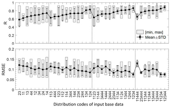
Figure 16.
R and RMSE statistics of the images fused by the LMGM PSS using different combinations of base data.
4. Discussion
This paper proposed a new fusion strategy, namely, the PSS, for selecting the optimal base data in spatiotemporal data fusion. The PSS was tested for the study area in the widely used ESTARFM and LMGM algorithms in the context of fusing MODIS and Landsat 8 OLI NDVI data. The results show that the PSS can reflect the spatiotemporal fusion accuracy and achieves higher accuracy than the NDS and HCS for both the ESTARFM and the LMGM algorithms.
The PSS provides several significant improvements over the existing NDS and HCS. First, the PSS combines the phenological similarity and seasonal symmetry to compute an indicative weight capable of identifying the optimal combination of base image pairs. The PSS weight was found to be linearly related to the Landsat image similarity and a very good indicator of the fusion accuracy for the ESTARFM and LMGM algorithms. Second, the PSS is simple and efficient. It is very flexible and therefore can adapt to different fusion algorithms. Particularly for the LMGM, the PSS can automatically determine whether to use one or two image pairs, which is very difficult for the NDS and HCS to accomplish. Third, the PSS provides a practical tool to quantify the temporal distribution of input image pairs, which enables us to identify the optimal combinations of image pairs.
The PSS performed much better than the NDS and HCS for land cover types with significant seasonal variations. For vegetation with nonsignificant phenological changes, e.g., evergreen coniferous forest, the influences of phenological similarity and seasonal symmetry can be neglected; the NDS and HCS may perform better in this case. For both the ESTARFM and the LMGM, the HCS achieved better results than the NDS in the study, which agrees with the results of [21] in the STARFM.
The phenological division is a major source of uncertainty for the PSS. The accurate division of phenological stages is important but is limited by two major factors. On the one hand, the phenological characteristics of the landscape vary greatly in space, while the PSS requires only one general division for base data selection. On the other hand, the phenological division relies on prior knowledge or coarse-resolution NDVI time series, which may be inconsistent with the real transitional dates at a fine resolution [38]. However, these uncertainties in the phenological division have limited impacts on the PSS. First, despite the abovementioned variation in phenological characteristics, the relative similarity between images among the four stages is widely applicable. Particularly, for both single- and double-season vegetation, stage 2 is most similar to stage 3, followed by stages 1 and 4. Normally, we recommend dividing the phenological stages based on the major vegetation type in the study area. Second, errors in determining the transitional dates have a limited influence on the PSS weights. For example, the uncertainty of ±20 days in the phenological transitional date would influence only the PSS weights within the same time interval of ±20 days. Only when the candidate image pair is in the same interval might the PSS result in bias in identifying the optimal combination of image pairs. To address this issue, we can apply the NDS when two candidate image pairs are both temporally near the prediction date. The PSS is particularly advantageous for large base-prediction time intervals, i.e., covering different phenological stages, which is very common for the cases of limited input data.
Several future improvements can be made to the PSS. First, the PSS performance was tested in a small study area that comprises mainly single-season forests. The phenological division of the PSS may be site-specific and may need to be adjusted for other study areas. Accordingly, the weighting scheme for phenological similarity may also need to be adjusted. Second, although the study area covers a small portion of double-season cropland, the phenological division was based mainly on the dominant type of vegetation, i.e., single-season forest. Hence, the PSS needs to be extended to more complex situations, such as landscapes that comprise mainly double-season vegetation. Third, the PSS in this study considers only gradual changes in the landscape caused by vegetation phenology. Therefore, further efforts may be exerted to integrate complex and sudden changes in the landscape into the PSS.
Moreover, this study focused primarily on improving the performance of spatiotemporal fusion algorithms with limited input data by optimizing the selection of base data. Other factors that might influence the spatiotemporal data fusion accuracy, such as the MODIS data quality and the consistency between MODIS and Landsat images [7,21,39,40,41], were not considered for simplicity. Such a simplification in base data selection is reasonable because the PSS, NDS, and HCS were compared on the same data basis. Nevertheless, further efforts could be made to integrate the consistency criterion into the PSS.
The PSS in this study was tested for blending Landsat 8 OLI and MODIS NDVI data. However, the PSS is also applicable for spatiotemporally fusing other coarse and fine images, e.g., Landsat 5/7 and MODIS data. Based on the phenological similarity between two dates, the PSS selects the most appropriate base date from all candidate dates for each prediction date. Similar as the NDS and the HCS [7], the PSS is also independent of specific satellite sensors.
Our conclusions regarding the influence of input data on the fusion accuracy are based on actual Landsat and MODIS images available in the Guanzhong region. However, due to the frequent occurrence of clouds, fog, haze, and rainfall, only three cloud-free Landsat images (i.e., DOY 129, 145, and 225) are available at stages 2 and 3. This prevents us from performing a complete investigation on the influence of the base data distribution since distribution patterns such as ‘2233’ are absent. However, in most cases, the images at stages 1 and 4 are easy to obtain due to the relatively infrequent occurrence of clouds and rain. Based on the available Landsat images at stages 1 or 4, one or more cloud-free Landsat images at stages 2 or 3 would greatly enhance the fusion accuracy. This conclusion is still valid and meaningful for practical applications in rainy and cloudy areas.
5. Conclusions
This study proposed a new similarity-based strategy, namely, the PSS, for base data selection in spatiotemporal data fusion algorithms with limited input data. The PSS computes a weight value, namely, the PSS weight, for identifying the optimal combination of base image pairs for each prediction date. To verify the validity of the PSS, the relationship between the PSS weight and image similarity/fusion accuracy was investigated. The performance of the PSS was compared with that of the commonly used NDS and HCS with limited input data. Finally, the influence of limited input base data on the performance of two fusion algorithms was examined. Particular emphasis was given to the influences of the number and temporal distribution of base data on the fusion accuracy. The main conclusions can be drawn as follows.
- (1)
- The base-prediction time interval has a nonlinear and complex relationship with the fusion accuracy using the ESTARFM and LMGM algorithms. Hence, the base-prediction time interval alone cannot explain the changes in fusion accuracy. The MODIS correlation has a linear relationship with, but is not a good indicator of the fusion accuracy due to its narrow value range. In contrast, the PSS weight has a wider range of 0~1 or 0~1.5 corresponding to cases involving one or two image pairs, respectively. We found a strong linear correlation between the PSS weight and actual Landsat image similarity (R = 0.925), which is much higher than the correlation between the MODIS image similarity and Landsat image similarity (R = 0.877). This confirms that the PSS readily captures the similarity between fine images on different dates and can serve as a good indicator for base data selection in spatiotemporal fusion algorithms.
- (2)
- The PSS achieves higher accuracy than the NDS and HCS in the ESTARFM and LMGM algorithms. For the ESTARFM algorithm, the predictability of the image pairs selected by the PSS is better than that of the pairs selected by the NDS and HCS. For the LMGM algorithm, using one image pair yields a higher accuracy than using two image pairs for both the NDS and the HCS. In general, LMGM-PSS produces systematically higher accuracies than LMGM-NDS-1, LMGM-NDS-2, LMGM-HCS-1, and LMGM-HCS-2, indicating that LMGM-PSS could combine the complementary strength of using one and two image pairs. Furthermore, LMGM-PSS is very flexible and can automatically determine whether to use one or two image pairs for a prediction date.
- (3)
- In the cases involving very limited input data, the timing of the base image pairs is much more important than the absolute number of base image pairs on the fusion accuracy using the PSS. Even with very limited data (Nin = 2), spatiotemporal data fusion could be highly accurate given appropriate temporal distribution patterns. An increase in the number of base image pairs does not necessarily improve the fusion accuracy, but including an additional image pair at a dissimilar phenological stage can significantly enhance the accuracy of year-round predictions. In general, base data that adequately cover the four phenological stages are more likely to produce a high fusion accuracy.
Author Contributions
Conceptualization, Y.W. and G.Y.; methodology, Y.W. and D.X.; software, Y.Z. and H.L.; data curation, Y.W.; writing—original draft preparation, Y.W.; writing—review and editing, Y.Z., D.X. and Y.C. All authors have read and agreed to the published version of the manuscript.
Funding
This research was funded by the National Natural Science Foundation of China (Grant No. 41901301), Natural Science Foundation of Shaanxi Province (Grant No. 2020JQ-739), Open Fund of State Key Laboratory of Remote Sensing Science (Grant No. OFSLRSS201922), and Doctoral Scientific Research Fund of Xi’an University of Science and Technology (Grant No. 2019QDJ006).
Institutional Review Board Statement
Not applicable.
Informed Consent Statement
Not applicable.
Data Availability Statement
This study was performed based on public-access data. The data that support the findings of this study are available from the corresponding author upon reasonable request.
Acknowledgments
We would like to thank Wanjuan Song and the anonymous reviewers for their insightful comments on this manuscript.
Conflicts of Interest
The authors declare no conflict of interest.
References
- Emelyanova, I.V.; McVicar, T.R.; Van Niel, T.G.; Li, L.T.; Van Dijk, A.I.J.M. Assessing the accuracy of blending Landsat–MODIS surface reflectances in two landscapes with contrasting spatial and temporal dynamics: A framework for algorithm selection. Remote Sens. Environ. 2013, 133, 193–209. [Google Scholar] [CrossRef]
- Gevaert, C.M.; García-Haro, F.J. A comparison of STARFM and an unmixing-based algorithm for Landsat and MODIS data fusion. Remote Sens. Environ. 2015, 156, 34–44. [Google Scholar] [CrossRef]
- Gao, F.; Masek, J.; Schwaller, M.; Hall, F. On the blending of the Landsat and MODIS surface reflectance: Predicting daily Landsat surface reflectance. IEEE Trans. Geosci. Remote Sens. 2006, 44, 2207–2218. [Google Scholar] [CrossRef]
- Zhu, X.; Cai, F.; Tian, J.; Williams, T.K.A. Spatiotemporal Fusion of Multisource Remote Sensing Data: Literature Survey, Taxonomy, Principles, Applications, and Future Directions. Remote Sens. 2018, 10, 527. [Google Scholar] [CrossRef]
- Hilker, T.; Wulder, M.A.; Coops, N.C.; Seitz, N.; White, J.C.; Gao, F.; Masek, J.G.; Stenhouse, G. Generation of dense time series synthetic Landsat data through data blending with MODIS using a spatial and temporal adaptive reflectance fusion model. Remote Sens. Environ. 2009, 113, 1988–1999. [Google Scholar] [CrossRef]
- Zhu, X.; Jin, C.; Feng, G.; Chen, X.; Masek, J.G. An enhanced spatial and temporal adaptive reflectance fusion model for complex heterogeneous regions. Remote Sens. Environ. 2010, 114, 2610–2623. [Google Scholar] [CrossRef]
- Wang, P.; Gao, F.; Masek, J.G. Operational Data Fusion Framework for Building Frequent Landsat-Like Imagery. IEEE Trans. Geosci. Remote Sens. 2014, 52, 7353–7365. [Google Scholar] [CrossRef]
- Cui, J.; Xin, Z.; Luo, M. Combining Linear Pixel Unmixing and STARFM for Spatiotemporal Fusion of Gaofen-1 Wide Field of View Imagery and MODIS Imagery. Remote Sens. 2018, 10, 1047. [Google Scholar] [CrossRef]
- Xie, D.; Zhang, J.; Zhu, X.; Pan, Y.; Liu, H.; Yuan, Z.; Yun, Y. An Improved STARFM with Help of an Unmixing-Based Method to Generate High Spatial and Temporal Resolution Remote Sensing Data in Complex Heterogeneous Regions. Sensors 2016, 16, 207. [Google Scholar] [CrossRef]
- Amorós-López, J.; Gómez-Chova, L.; Alonso, L.; Guanter, L.; Zurita-Milla, R.; Moreno, J.; Camps-Valls, G. Multitemporal fusion of Landsat/TM and ENVISAT/MERIS for crop monitoring. Int. J. Appl. Earth Obs. Geoinf. 2013, 23, 132–141. [Google Scholar] [CrossRef]
- Zurita-Milla, R.; Clevers, J.G.P.W.; Schaepman, M.E. Unmixing-Based Landsat TM and MERIS FR Data Fusion. IEEE Geosci. Remote Sens. Lett. 2008, 5, 453–457. [Google Scholar] [CrossRef]
- Zurita-Milla, R.; Gómez-Chova, L.; Guanter, L.; Clevers, J.G.P.W.; Camps-Valls, G. Multitemporal Unmixing of Medium-Spatial-Resolution Satellite Images: A Case Study Using MERIS Images for Land-Cover Mapping. IEEE Trans. Geosci. Remote Sens. 2011, 49, 4308–4317. [Google Scholar] [CrossRef]
- Zurita-Milla, R.; Kaiser, G.; Clevers, J.G.P.W.; Schneider, W.; Schaepman, M.E. Downscaling time series of MERIS full resolution data to monitor vegetation seasonal dynamics. Remote Sens. Environ. 2009, 113, 1874–1885. [Google Scholar] [CrossRef]
- Xue, J.; Leung, Y.; Fung, T. A Bayesian Data Fusion Approach to Spatio-Temporal Fusion of Remotely Sensed Images. Remote Sens. 2017, 9, 1310. [Google Scholar] [CrossRef]
- Song, H.; Huang, B. Spatiotemporal Satellite Image Fusion through One-Pair Image Learning. IEEE Trans. Geosci. Remote Sens. 2013, 51, 1883–1896. [Google Scholar] [CrossRef]
- Song, H.; Liu, Q.; Wang, G.; Hang, R.; Huang, B. Spatiotemporal Satellite Image Fusion Using Deep Convolutional Neural Networks. IEEE J. Sel. Top. Appl. Earth Obs. Remote Sens. 2018, 11, 1–9. [Google Scholar] [CrossRef]
- Wei, J.; Wang, L.; Liu, P.; Song, W. Spatiotemporal Fusion of Remote Sensing Images with Structural Sparsity and Semi-Coupled Dictionary Learning. Remote Sens. 2016, 9, 21. [Google Scholar] [CrossRef]
- Bo, P.; Meng, Y.; Su, F. An Enhanced Linear Spatio-Temporal Fusion Method for Blending Landsat and MODIS Data to Synthesize Landsat-Like Imagery. Remote Sens. 2018, 10, 881. [Google Scholar] [CrossRef]
- Zhu, X.L.; Helmer, E.H.; Gao, F.; Liu, D.S.; Chen, J.; Lefsky, M.A. A flexible spatiotemporal method for fusing satellite images with different resolutions. Remote Sens. Environ. 2016, 172, 165–177. [Google Scholar] [CrossRef]
- Chen, Y.; Cao, R.Y.; Chen, J.; Zhu, X.L.; Zhou, J.; Wang, G.P.; Shen, M.G.; Chen, X.H.; Yang, W. A New Cross-Fusion Method to Automatically Determine the Optimal Input Image Pairs for NDVI Spatiotemporal Data Fusion. IEEE Trans. Geosci. Remote Sens. 2020, 58, 5179–5194. [Google Scholar] [CrossRef]
- Xie, D.; Gao, F.; Sun, L.; Anderson, M. Improving Spatial-Temporal Data Fusion by Choosing Optimal Input Image Pairs. Remote Sens. 2018, 10, 1142. [Google Scholar] [CrossRef]
- Olexa, E.M.; Lawrence, R.L. Performance and effects of land cover type on synthetic surface reflectance data and NDVI estimates for assessment and monitoring of semi-arid rangeland. Int. J. Appl. Earth Obs. Geoinf. 2014, 30, 30–41. [Google Scholar] [CrossRef]
- Liu, M.; Yang, W.; Zhu, X.L.; Chen, J.; Chen, X.H.; Yang, L.Q.; Helmer, E.H. An Improved Flexible Spatiotemporal DAta Fusion (IFSDAF) method for producing high spatiotemporal resolution normalized difference vegetation index time series. Remote Sens. Environ. 2019, 227, 74–89. [Google Scholar] [CrossRef]
- Ju, J.; Roy, D.P. The availability of cloud-free Landsat ETM+ data over the conterminous United States and globally. Remote Sens. Environ. 2008, 112, 1196–1211. [Google Scholar] [CrossRef]
- Wang, Y.; Xie, D.; Liu, S.; Hu, R.; Li, Y.; Yan, G. Scaling of FAPAR from the Field to the Satellite. Remote Sens. 2016, 8, 310. [Google Scholar] [CrossRef]
- Wang, Y.; Xie, D.; Li, X. Universal scaling methodology in remote sensing science by constructing geographic trend surface. J. Remote Sens. 2014, 18, 1139–1146. (in Chinese). [Google Scholar]
- Wang, Y.; Yan, G.; Hu, R.; Xie, D.; Chen, W. A Scaling-Based Method for the Rapid Retrieval of FPAR from Fine-Resolution Satellite Data in the Remote-Sensing Trend-Surface Framework. IEEE Trans. Geosci. Remote Sens. 2020, 58, 7035–7048. [Google Scholar] [CrossRef]
- Rao, Y.; Zhu, X.; Chen, J.; Wang, J. An Improved Method for Producing High Spatial-Resolution NDVI Time Series Datasets with Multi-Temporal MODIS NDVI Data and Landsat TM/ETM+ Images. Remote Sens. 2015, 7, 7865–7891. [Google Scholar] [CrossRef]
- Hu, S.; Mo, X.; Lin, Z. Optimizing the photosynthetic parameter Vcmax by assimilating MODIS-fPAR and MODIS-NDVI with a process-based ecosystem model. Agric. For. Meteorol. 2014, 198-199, 320–334. [Google Scholar] [CrossRef]
- Gamon, J.A.; Huemmrich, K.F.; Stone, R.S.; Tweedie, C.E. Spatial and temporal variation in primary productivity (NDVI) of coastal Alaskan tundra: Decreased vegetation growth following earlier snowmelt. Remote Sens. Environ. 2013, 129, 144–153. [Google Scholar] [CrossRef]
- Meng, J.; Du, X.; Wu, B. Generation of high spatial and temporal resolution NDVI and its application in crop biomass estimation. Int. J. Digit. Earth 2013, 6, 203–218. [Google Scholar] [CrossRef]
- Jarihani, A.A.; McVicar, T.R.; Niel, T.G.V.; Emelyanova, I.V.; Callow, J.N.; Johansen, K. Blending Landsat and MODIS Data to Generate Multispectral Indices: A Comparison of “Index-then-Blend” and “Blend-then-Index” Approaches. Remote Sens. 2014, 6, 9213–9238. [Google Scholar] [CrossRef]
- Tian, F.; Wang, Y.; Fensholt, R.; Wang, K.; Zhang, L.; Huang, Y. Mapping and Evaluation of NDVI Trends from Synthetic Time Series Obtained by Blending Landsat and MODIS Data around a Coalfield on the Loess Plateau. Remote Sens. 2013, 5, 4255–4279. [Google Scholar] [CrossRef]
- Chen, X.H.; Liu, M.; Zhu, X.L.; Chen, J.; Zhong, Y.F.; Cao, X. “Blend-then-Index” or “Index-then-Blend”: A Theoretical Analysis for Generating High-resolution NDVI Time Series by STARFM. Photogramm. Eng. Remote Sens. 2018, 84, 66–74. [Google Scholar] [CrossRef]
- Wulder, M.A.; Loveland, T.R.; Roy, D.P.; Crawford, C.J.; Masek, J.G.; Woodcock, C.E.; Allen, R.G.; Anderson, M.C.; Belward, A.S.; Cohen, W.B.; et al. Current status of Landsat program, science, and applications. Remote Sens. Environ. 2019, 225, 127–147. [Google Scholar] [CrossRef]
- Markham, B.L.; Storey, J.C.; Williams, D.L.; Irons, J.R. Landsat sensor performance: History and current status. IEEE Trans. Geosci. Remote Sens. 2004, 42, 2691–2694. [Google Scholar] [CrossRef]
- Vermote, E.; Justice, C.; Claverie, M.; Franch, B. Preliminary analysis of the performance of the Landsat 8/OLI land surface reflectance product. Remote Sens. Environ. 2016, 185, 46–56. [Google Scholar] [CrossRef]
- Zhang, X.; Wang, J.; Gao, F.; Liu, Y.; Schaaf, C.; Friedl, M.; Yu, Y.; Jayavelu, S.; Gray, J.; Liu, L. Exploration of scaling effects on coarse resolution land surface phenology. Remote Sens. Environ. 2017, 190, 318–330. [Google Scholar] [CrossRef]
- Walker, J.J.; De Beurs, K.M.; Wynne, R.H.; Gao, F. Evaluation of Landsat and MODIS data fusion products for analysis of dryland forest phenology. Remote Sens. Environ. 2012, 117, 381–393. [Google Scholar] [CrossRef]
- Gao, F.; Anderson, M.C.; Zhang, X.; Yang, Z.; Alfieri, J.G.; Kustas, W.P.; Mueller, R.; Johnson, D.M.; Prueger, J.H. Toward mapping crop progress at field scales through fusion of Landsat and MODIS imagery. Remote Sens. Environ. 2017, 188, 9–25. [Google Scholar] [CrossRef]
- Gao, F.; He, T.; Masek, J.G.; Shuai, Y.; Schaaf, C.; Wang, Z. Angular Effects and Correction for Medium Resolution Sensors to Support Crop Monitoring. IEEE J. Sel. Top. Appl. Earth Obs. Remote Sens. 2014, 7, 4480–4489. [Google Scholar] [CrossRef]
Publisher’s Note: MDPI stays neutral with regard to jurisdictional claims in published maps and institutional affiliations. |
© 2021 by the authors. Licensee MDPI, Basel, Switzerland. This article is an open access article distributed under the terms and conditions of the Creative Commons Attribution (CC BY) license (http://creativecommons.org/licenses/by/4.0/).