The Impact of the Selection of Exogenous Variables in the ANFIS Model on the Results of the Daily Load Forecast in the Power Company

Abstract

Forecasting of daily loads is crucial for the Distribution System Operators (DSO). Contemporary short-term load forecasting models (STLF) are very well recognized and described in numerous articles. One of such models is the Adaptive Neuro-Fuzzy Inference System (ANFIS), which requires a large set of historical data. A well-recognized issue both for the ANFIS and other daily load forecasting models is the selection of exogenous variables. This article attempts to verify the statement that an appropriate selection of exogenous variables of the ANFIS model affects the accuracy of the forecasts obtained ex post. This proposal seems to be a return to the roots of the Polish econometrics school and the use of the Hellwig method to select exogenous variables of the ANFIS model. In this context, it is also worth asking whether the use of the Hellwig method in conjunction with the ANFIS model makes it possible to investigate the significance of weather variables on the profile of the daily load in an energy company. The functioning of the ANFIS model was tested for some consumers exhibiting high load randomness located within the area under supervision of the examined power company. The load curves featuring seasonal variability and weekly similarity are suitable for forecasting with the ANFIS model. The Hellwig method has been used to select exogenous variables in the ANFIS model. The optimal set of variables has been determined on the basis of integral indicators of information capacity H. Including an additional variable, i.e., air temperature, has also been taken into consideration. Some results of ex post daily load forecast are presented.

1. Introduction

Forecasting of load in the power system and subsystems is a process of determining future values of time-series based on current and historical values. The forecast horizon may apply either to a single step or to many steps. In the case of long-term forecasts, the length of the step is usually a year, medium-term forecasts a month or day, short-term forecast an hour, and for very short-term forecasts a second (this is the case of real time forecasting).

Short-term load forecasting (STLF) is used for operation and planning the power system and subsystems. Forecasts are necessary for a deregulated energy market in order to plan and implement management operations. These types of forecasts are also necessary at the level of the distribution system operators (DSO) and their sections, i.e., distribution companies. Load profiles at the distribution companies’ level are characterized by significant discrepancies related to unstable behavior of the consumers with significant power demand, which places major challenges before the forecasting models for the regions within the distribution company area.

The paper is an attempt to use the forecasting model that minimizes mean absolute forecast error, but at the same time it addresses the problem of developing an algorithm for selection of variables. Moreover, an analysis of the impact of exogenous variables set on the model accuracy is carried out. Factors that affect the load can be divided into a group specifying the behavior patterns of consumers during a day and a week (time of day, day of a week, Sunday and holiday), another group specifying the type of consumer (residential, municipal, industrial, etc.) and a group specifying weather conditions (temperature, humidity, cloudiness, wind, etc.) [1,2]. Considering the above, one may suspect that the selection of the forecasting model form is strongly affected by daily, weekly and annual variability of a cyclic nature [3]. This feature should be present in short-term forecasting. In the Polish climatic zone, only ambient temperature shows a significant impact on the load profile in the power system and subsystems [2], even though weather conditions are used in many generally applied models [4,5]. The main issue related to the short-term forecasting is the selection of the input quantities in the model [6,7,8]. The paper focuses on this issue and the impact of the variables on the forecasting process using a model utilizing cyclic changes of the input variables.

This paper puts forth an original approach to forecasting electricity consumption, combining the Hellwig method of selecting a set of exogenous variables with the ANFIS model. It also demonstrates that introducing climate-related variables does not necessarily improve the accuracy of forecasting. The usefulness of ANFIS in modeling periodical processes with random deviations has already been proven in a number of publications. This paper additionally proves that the accuracy of the ANFIS model largely depends on the character of input data. In selected applications, such as the example presented in the software Matlab R2020b, the time series was generated on the basis of the Mackey-Glass time-delay differential equation. The MAPE of the ex post is about 3.5%. The research presented here aims to demonstrate that an increase in random deviations within random exogenous variables of the ANFIS model causes a significant increase in the MAPE of ex post forecasts.

2. Classification of STLF Methods and Forecasting Experience

There are many short-term forecasting methods used to forecast power system and subsystems loads, including but not limited to:

• Linear regression models (auto-regression model of a row p AR(p), moving average model of a row q MA(q), auto-regression and moving average model (p,q) ARMA(p,q), model GARCH),
• Artificial neural networks ANN model,
• Fuzzy logic models,
• Adaptive Neuro-Fuzzy Inference System (ANFIS),
• Data Mining techniques and Support Vector Machines (SVM),
• Wavelet pre-filtering based on ANN and fuzzy models.

In short-term forecasting, ref. [9] various methods based on linear regression are commonly applied due to their simplicity, ease of implementation and reliable results. The regression techniques estimate relationships between exogenous variables and the endogenous variable. They include various variables such as historical loads, weather variables or calendar variables. The review of forecasting method given in Ref. [10] shows that usually the regression factors are estimated based on the least square method.

If chronological series of loads in the power system is characterized with periodic cycles, it is justified to use the following methods for time-series analysis: auto-regression (AR) models and their variants, exponential smoothing models and kernel density estimation (KDE) algorithms. In the AR row model p, identified as AR(p), the load at the instant of time t is the sum of linear combination of historical loads at time instants p and stochastic error. The AR(p) model parameters can be estimated using the Burg method. Some modifications of the AR models with the aggregated load profiles are presented by e.g., Weron [3] and Taylor and McSharry [11].

In 1970, the Box and Jenkins book (former edition of Box et al. [12]) was published for the first time with the description of the autoregressive integrated moving average (ARIMA) time series models that are used to forecast the loads, including such components as trend, season changes and some irregularities. The moving average model (MA) forecasts the endogenous variable as a sum of the expected value of this variable, linear combination of previous errors of the row q and random noise term. The paper of Singh et al. [9] is one of most interesting comprehensive papers on ARMA model application in forecasting the loads. In the aforementioned paper, the (S)ARMA model has been developed by additional exogenous variables such as temperature, wind, etc., giving rise to the models (S)ARIMAX or (S)ARMAX.

A model that takes into account the annual as well as weekly and daily variables is the model of exponential equalizing, also known as Holt-Winters model [13]. Good results are also obtained using the extension of this model, known as Holt-Winters-Taylor model [14,15], which includes the impact of temperature on the load.

A popular forecasting technique, also used for forecasting the load, is the kernel density estimation (KDE), e.g., in [16] a forecasting model is provided of the load profile of a single consumer of low voltage. A similar topic is discussed in the paper by Dudek [17].

The regression models include also the k-nearest neighbor (kNN) model. The algorithm searches for similar profiles among historical data, considering the Euclidean measure of distance. The forecast is an arithmetic mean of k neighbors. Substituting the Euclidean measure with error estimation p, and the arithmetic mean with the permutation consolidation of the corrected mean, the adjusted feature aware k-nearest neighbor (AFkNN) is derived.

When the load trend is non-linear, acceptable results can be achieved using the following forecasting techniques: fuzzy logic [18] and fuzzy neural networks [19].

A novel method is the improvement of STLF effectiveness through the use of the long short-term memory (LSTM) and GA algorithm to forecast hourly load of the following day [20].

A method that enhances accuracy of the forecasting model using the artificial neural networks is the selection of similar days using the reinforcement learning algorithm based on the Deep Q-Network technique [21].

An interesting approach is represented by algorithms using machine-type learning, i.e., an automatic system that is able to learn based on available data and gain new knowledge [22,23]. Usually, machine-type learning leads to the selection of the most appropriate forecasting model, as proven in, e.g., [23]. The machine-type learning also uses an adaptive neural fuzzy inference system (ANFIS) to very short-term wind forecasting [24].

Hybrid models are becoming more important and combine various forecasting techniques, e.g., [25,26]. A hybrid algorithm improving the forecasting accuracy is presented in [26]. In order to select the input vector, the non-dominated sorting genetic algorithm II (NSGA II) was used that includes a multi-layer perception neural network (MLPNN). The result of NSGA II, i.e., the best combination of input data is used in the adaptive neuro-fuzzy inference system (ANFIS).

Modern forecasting methods (artificial neural network, evolution algorithms, fuzzy logic) require numerous sets, usually to perform the learning process and then to verify the adopted model. For analyses of time curves of the load in the power subsystems, the paper uses the description of load variability in the power system. The methodology presented in Section 5 is used as a tool for constructing the ANFIS model. The key issue in short-term forecasting is the selection of model input variables. The paper deals with this issue and the influence of variables, and more precisely an additional variable, i.e., ambient temperature, on the accuracy of the forecasting process with a model using cyclic changes of input variables.

3. Description of the Load Variability

The main reason for the phenomenon called load variability is the behavior of the customers, conditioned by the season, tradition and habits as well as the nature of the work that shape the schedule of a working day and a holiday. The system load is affected by both non-accidental and random factors [27]. The main non-accidental factors are: geographical location of the area under consideration and its climate, change of the sun radiation incidence angle, changes of the time of sunrise and sunset as well as the features of the power system such as reception structure, dynamics of the economy development, statutory length of a work day and the system of working shifts applicable within a given country [1,28,29]. The random factors include: changes of temperature, rainfall, cloudiness, wind rate, failures in the power system, changes in the consumers structure, etc.

Consumer load time series can be represented as a random function [1,2]. The power system load is a result of a superposition of individual load profiles of the consumers and represents a sum of random functions. This is to underline that they are subject to increase within a year that is also of random character.

Behavior patterns of citizens, relationship of such patterns with changing seasons, traditions and habits, as well as the nature of the work performed by persons that control the schedule of a working day and holiday affect the loads in the power system and are the main cause of the load variability phenomenon.

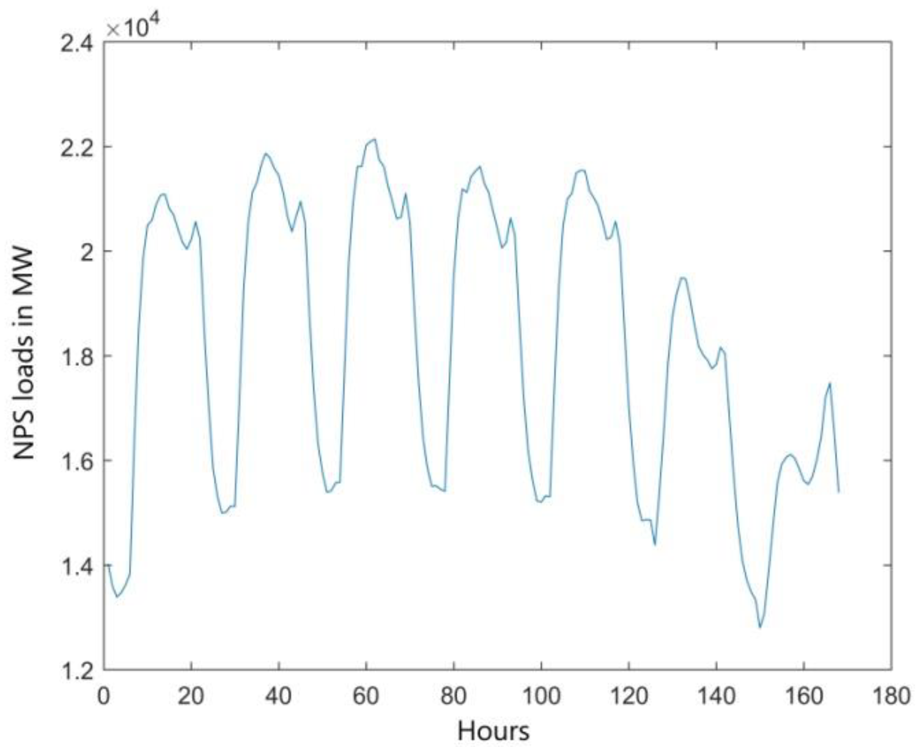
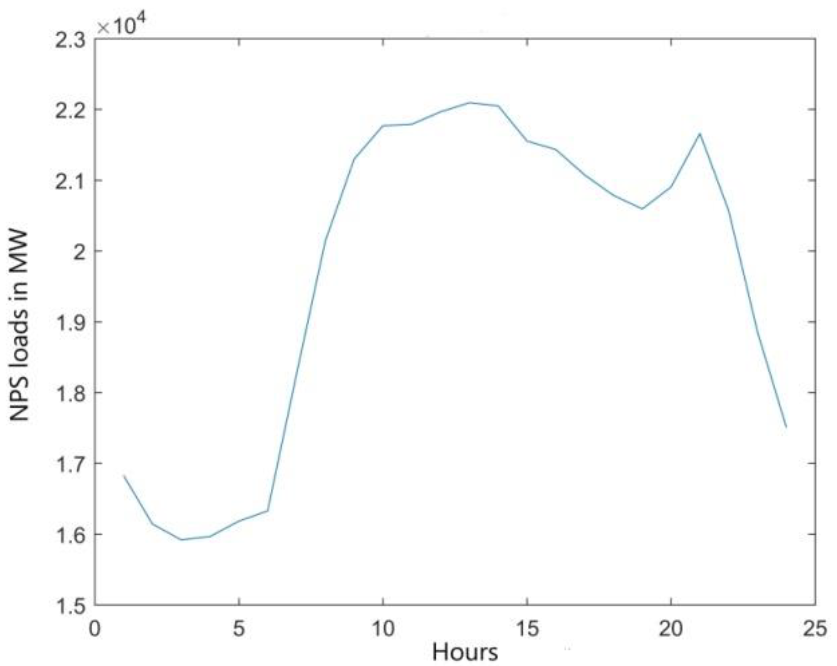
The daily load is affected by work schedule and household activities (Figure 1). The nightly loads drop is noticeable from 11 p.m. to 6 a.m. Most of the working population starts their professional activities between 6 a.m. and 10 a.m. and within this period there is a significant increase in power consumption. Reduction of the load takes place at the turn of the working shifts, i.e., 2 p.m. This is caused by shutting down some of the electricity equipment at industrial plants. In the Polish power system, there is a clear evening peak after people return home from work. So far, it has been attributed to an increase in the use of lighting. Along with technological changes, there are evolutionary changes in the daily load profile, e.g., related to more popular use of air-conditioning.

A different pattern of load reduction on Saturday is presented in Figure 2, which is related to the fact that the working week in Poland is five days long. On Sunday, only the industry of continuous production mode and some of the institutions and public utility companies, hospitals, and transport are working, thus the power demand is much lower when compared to the remaining week days.

The forecasting process capitalizes on the regularities of the daily and weekly load reduction. Stable changes in the remaining weeks of the year cause modern load forecasting methods in the Polish power system to achieve average percentage absolute errors below 2%. However, completely different and burdened with major problems is the forecasting at the level of distribution companies covering small regions. This load is characterized by much more instability of consumers’ behavior and the load profiles may significantly differ from the shapes of the national load curves. The paper uses the data of the power company load, which is difficult to forecast load due to significant random deviations.

4. Statistical Data

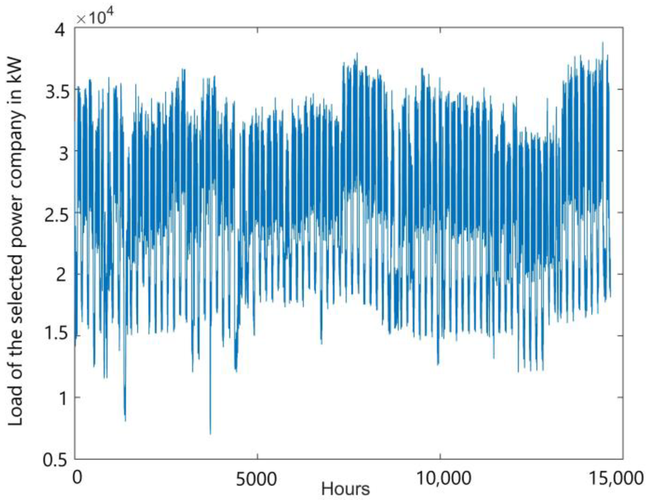
Statistical data used in the paper concerns hourly loads from a roughly two-year-long period at the selected power company. The power company loads are characterized by noticeable random fluctuation (Figure 3).

The studies have been performed both for the full chronological series and one limited to a selected weekday. When analyzing weekly variability (Figure 2), lower demand for electrical power on Sundays and holidays can be clearly seen. Working days of a week show a significant similarity. Forecasting models were constructed for each day of the week. Wednesday is a typical working day in Poland, therefore the analysis presented in Section 7 refers to that day, but

Table 1. Integral capacities of information carriers for the selected sets of exogenous variables.

No. of Set	Endogenous Variable and Exogenous Variables	Integral Capacity of Information Carriers Hm
		Mon	Tues	Wed	Thurs	Fri	Sat	Sun
1	X(t + 24)X(t) X(t − 24) X(t − 48) θ(t)	0.535	0.249	0.371	0.358	0.396	0.716	0.349
2	X(t + 24)X(t) X(t − 24) θ(t)	0.466	0.216	0.364	0.347	0.352	0.666	0.334
3	X(t + 24)X(t) θ(t)	0.413	0.198	0.299	0.334	0.341	0.587	0.307
4	X(t + 24)X(t) X(t − 24) X(t − 48) X(t − 72)	0.543	0.255	0.372	0.363	0.399	0.746	0.336
5	X(t + 24)X(t) X(t − 24) X(t − 48)	0.545	0.261	0.379	0.355	0.404	0.743	0.331
6	X(t + 24)X(t) X(t − 24)	0.489	0.234	0.378	0.349	0.367	0.710	0.326

and

Table 2. MAPEs for ex post forecasts of loads.

No. of Set	Endogenous Variable and Exogenous Variables	Mean Absolute Percentage Error MAPE [%]
		Mon	Tues	Wed	Thurs	Fri	Sat	Sun
1	X(t + 24)X(t) X(t − 24) X(t − 48) θ(t)	IM	IM	IM	11.32	IM	IM	IM
2	X(t + 24)X(t) X(t − 24) θ(t)	11.08	10.60	8.95	9.46	8.48	10.14	8.23
3	X(t + 24)X(t) θ(t)	11.29	10.91	9.12	9.68	8.81	10.11	8.70
4	X(t + 24)X(t) X(t − 24) X(t − 48) X(t − 72)	IM	IM	IM	IM	IM	9.93	9.01
5	X(t + 24)X(t) X(t − 24) X(t − 48)	10.57	10.46	8.42	8.78	IM	9.39	7.86
6	X(t + 24)X(t) X(t − 24)	10.70	10.42	8.30	8.95	8.45	9.74	8.40
	Naive forecast	11.41	11.59	9.49	9.55	9.11	10.59	9.07

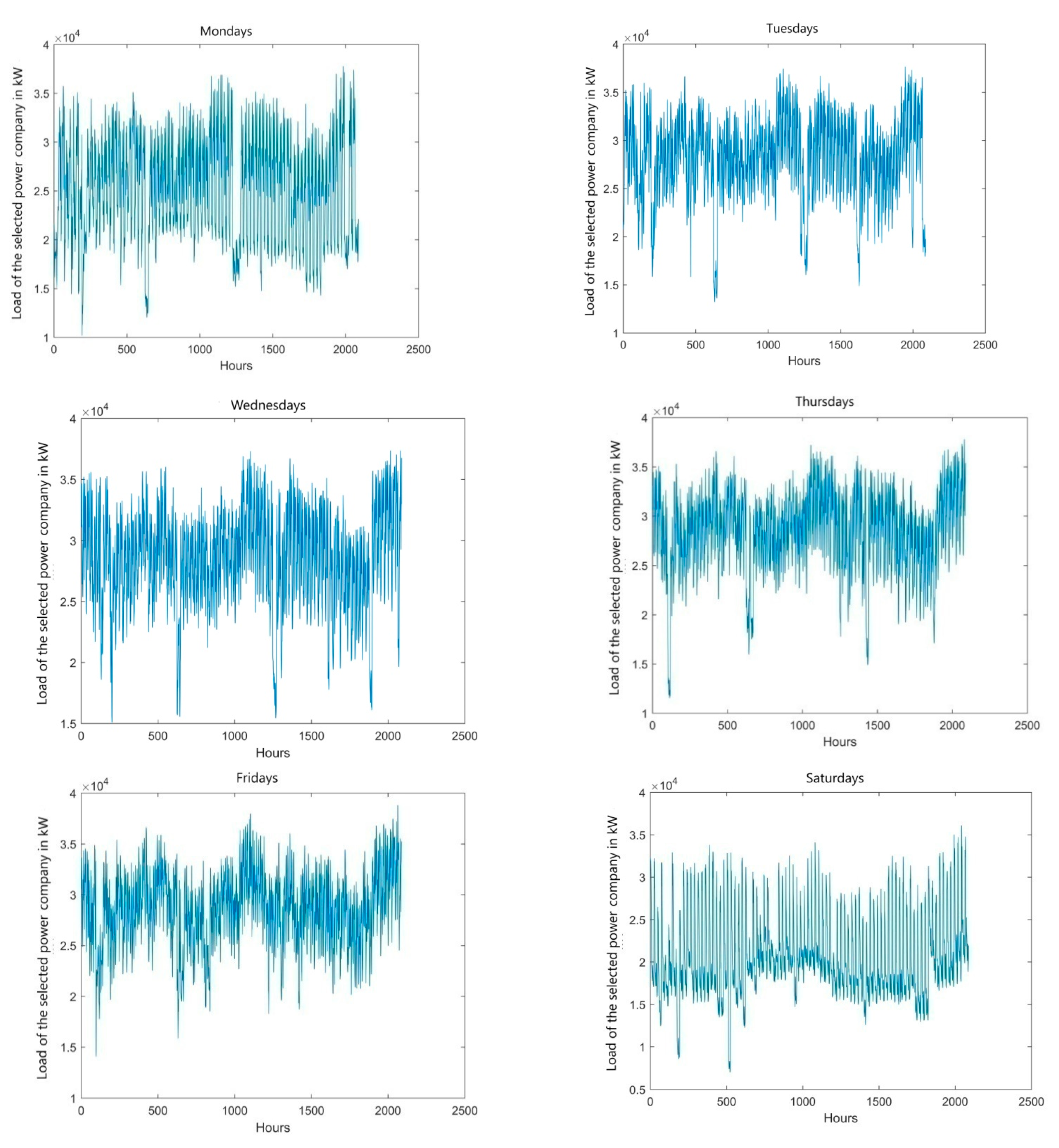
IM-Inadequate Model (means that the construction of a model that gives an ex post forecast better than the naive model has failed).

present the results also for the other days of the week. For each day of the week, a set was created with a number seven times smaller than the input chronological series. The new set is made of only 24-h series of subsequent days of the week and presented in Figure 4. The analysis of the load curves in Figure 4 indicates the special nature of the load profiles of the selected power company, because one can observe random disturbances of significant values in the time series.

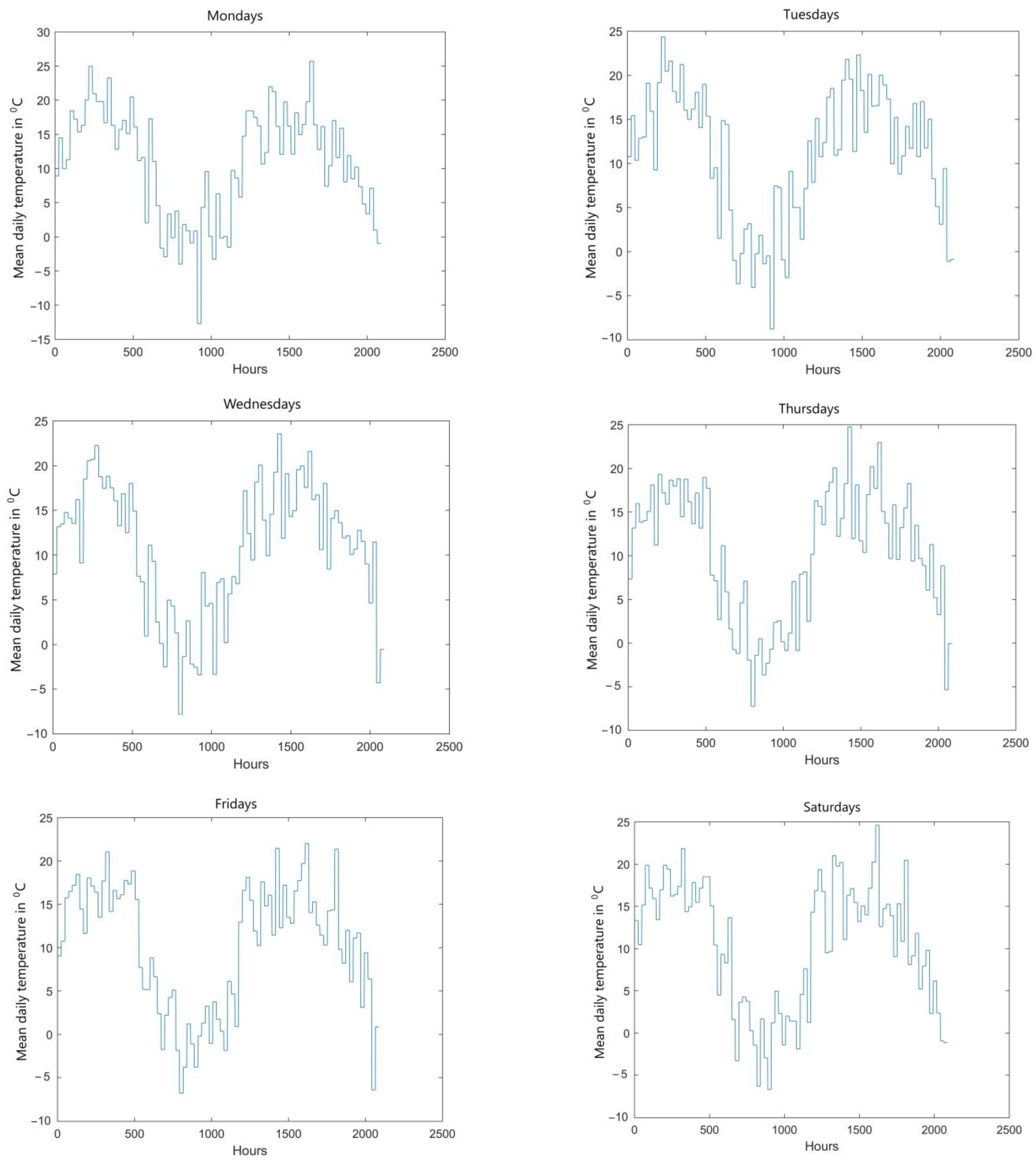
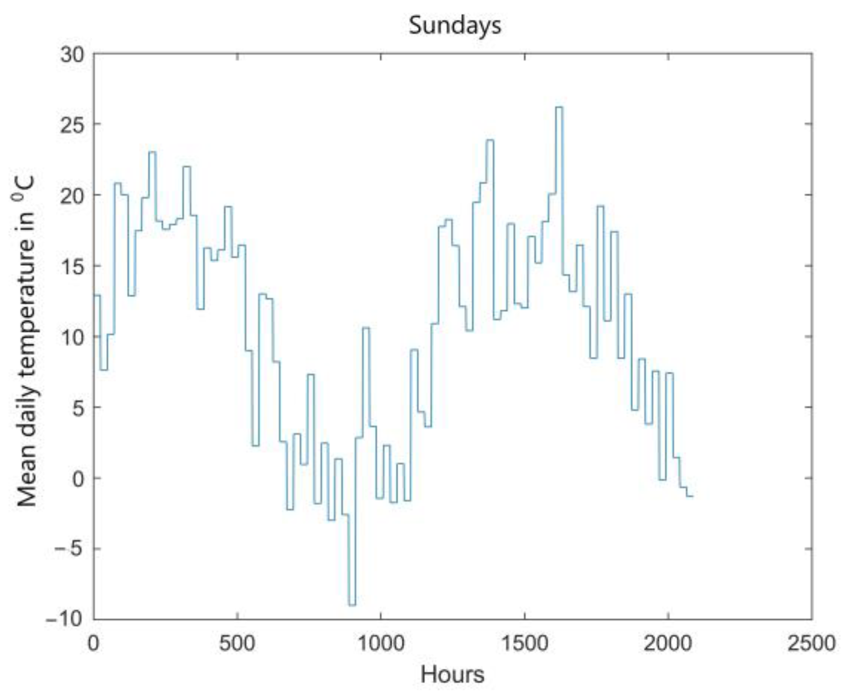
The load curve is slightly affected by weather conditions, the most important parameter of which is ambient temperature. For the load curves presented in Figure 4, curves of mean daily temperatures corresponding to subsequent days of the week were developed (Figure 5).

It can be remarked that there exists a contradictory trend between the load of the power company and the ambient temperature. Within the periods of temperature drop, higher electrical power demand is noticed, however the studies in Poland [1,2] show that temperature is not the only factor affecting the demand increase. The power load changes are also influenced by, for example, religious, sports and cultural events broadcast in real time by the mass media. The aim of the research is to verify the thesis about the significance of the impact of temperature on the load profiles.

5. Method of the Exogenous Variables Selection

5.1. Review of Methods

Many sources [7,8,30,31,32] provide descriptions of methods for selecting exogenous variables for econometric models. Selection of suitable subsets of variables can be made in order to show the cause and effect relationships, to improve forecast accuracy, to eliminate unimportant variables (noise reduction) or to reduce the modeling time. Current methods of variable selection are based on both multidimensional regression and simultaneous methods. The most common methods include: All Subset Models (ASM), Sequential Search (SS), StepWise regression methods (SW) based on the strategies such as Forward Selection (FS) and Backward Elimination (BE), Genetic Algorithms (GAs), Particle Swarm Optimization (PSO), Ant Colony Optimization (ACO), Least Absolute Shrinkage and Selection Operator (LASSO), Elastic Net as well as Variable Importance on Partial Least Squares (PLS) projections (VIP).

The method of All Subset Models (ASM) [8] consists in analyzing the models of all combinations from among n variables, i.e., 2ⁿ − 1 models. The method leads to the selection of the best subset of variables however, it is unsuitable for a large number of variables due to calculation time.

Sequential Search (SS) is a simple method of selection of the optimum subset of variables into a form of a model of specified number of variables [31]. Each next variable is selected by substituting it with the remaining variables and selecting the best one according to the adopted criterion.

StepWise regression method (SW) is one of the most commonly applied ones [31,32]. Using the Forward Selection (FS) strategy, the method starts with a model of dimension 0 and the next variables that meet the defined criterion are added. Usually, the variable selected at the next step is to minimize the Residual Sum of Squares (RSS), which enables estimating the F-Snedecor test that compares the models with p and p + j variables.

In the case of the Backward Elimination (BE), the algorithm starts with the p-dimensional model (where p is the maximum number of variables). During the next steps, unnecessary variables are eliminated to minimize the increase of RSS, tested using the F-Snedecor test. In modern algorithms, the F-test is replaced by minimization of other functions, e.g., the Akaike Information Criterion (AIC) [33].

Within recent years, methods using artificial intelligence become more and more common, e.g., Genetic Algorithms (GAs) [34,35], Particle Swarm Optimization (PSO) [36] or Ant Colony Optimization (ACO) [37]. The aforementioned algorithms were first used as optimization methods, however they were adapted to perform the selection of exogenous variables in the models.

The LASSO method belongs to the regression methods and was developed by R. Tibshirani in 1996 [38]. This method minimizes RSS with an additional condition that checks whether the sum of absolute values of factors is less than the assumed value. This provides the grounds for the selection of a set of variables because some of the regression factors assume values equal to 0.

The extension of the LASSO method when combined with the Ridge regression method results in the Elastic Net method as proposed by Zou and Hastie in 2005 [39]. The additional condition consists of a sum of absolute values of factors and the sum of the components squares. Such design of the criterion provides good selection results of variables strongly correlated with each other.

The Variables Importance Projections (VIP) method is based on the Canonical Powered Partial Least Squares (CPPLS) [40]. For each variable, the VIP factor is defined and the selection consists in removing variables with VIP value less that the defined criterion value (usually equal to 1, because the average VIP mean is 1).

5.2. Hellwig Method Algorithm

Many sources [7,8] provide descriptions of the selection of variables for econometric models. Methods for linear models or those that can be reduced to linear, single-equation methods are best developed. The basic postulate concerning the variables-strong correlation between each explaining and explained variable and at the same time a weak correlation between the explaining variables cause most of variable selection methods to avail of some versions of the linear correlation. A solution found to be an optimal one depends on the lowest number of mutually uncorrelated explaining variables. The explaining variables are as maximally correlated as possible with the explained variable. This general definition translates in the literature to a set of a dozen, and after a few modifications, a few dozen methods of variables selection [6].

The Hellwig method of integral information capacity is one of the most effective and at the same time simple methods according to [6,7]. This method won the greatest recognition among econometricians performing empirical studies.

The starting point here is estimation of the matrix R and vector R₀. The matrix R corresponds to a matrix of correlation factors between individual k explaining variables that may be expressed as follows:

$${{\displaystyle R}}_{}=\left[\begin{array}{cccccc}1& {{\displaystyle r}}_{12}& .& .& .& {{\displaystyle r}}_{1k}\\ {{\displaystyle r}}_{21}& 1& .& .& .& {{\displaystyle r}}_{2k}\\ .& .& 1& .& .& .\\ .& .& .& 1& .& .\\ .& .& .& .& 1& .\\ {{\displaystyle r}}_{k1}& {{\displaystyle r}}_{k2}& .& .& .& 1\end{array}\right].$$

(1)

However, vector R₀ is a vector of correlation factors between the explained variable and the following explaining variables. This vector can be expressed based on the matrix using the following equation:

$${{\displaystyle R}}_0=\left[\begin{array}{c}{{\displaystyle r}}_1\\ {{\displaystyle r}}_2\\ .\\ .\\ .\\ {{\displaystyle r}}_k\end{array}\right]$$

(2)

Then, the following calculations are performed of the so-called individual capacities of information carriers X_j of endogenous variable Y composed of different combinations of elements of a given explaining set of variables. It is known that the general number of these combinations is 2^k–1. The variable X_j is the better carrier of information of the Y variable, the closer to one is the linear correlation factor r_j of the module. Note that the variable X_j is the clear information carrier only when it is not correlated with other explaining variables. However, when the X_j variable is correlated with them, we assume that X_j is a contaminated information carrier of endogenous variable Y.

Contamination of an individual information carrier X_j is the quantity:

$${{\displaystyle g}}_j=\frac{1}{k-1}{\displaystyle \sum _{i\ne j}\left|{{\displaystyle r}}_{ij}\right|}$$

(3)

It may be easily checked that the inequality 0 ≤ g_j ≤1 is always fulfilled, wherein g_j = 0, when X_j is a clear information carrier of variable Y and g_j = 1, when information carrier contamination is complete.

Individual capacity of the information carrier X_j of variable Y is calculated using the following equation:

$${{\displaystyle h}}_j=\frac{{{\displaystyle r}}_j^2}{1+{\displaystyle \sum _{i\ne j}\left|{{\displaystyle r}}_{ij}\right|}}=\frac{{{\displaystyle r}}_j^2}{1+\left(k-1\right){{\displaystyle g}}_j}\left(i,j=1,\dots ,k;i\ne j\right).$$

(4)

In turn, the following equation is used to calculate the integral capacity of information carriers:

$${{\displaystyle H}}_m={\displaystyle \sum _{j=1}^k{{\displaystyle h}}_j}={\displaystyle \sum _{j=1}^k\frac{{{\displaystyle r}}_j^2}{1+{\displaystyle \sum _{i\ne j}\left|{{\displaystyle r}}_{ij}\right|}}}\left(m=1,2,\dots ,2^k-1\right)$$

(5)

It is possible to demonstrate that the H_m parameter is a standardized quantity in the range of 0 < H_m < 1. If this capacity is close to one, it means that the variables constituting a given combination provide almost a complete resource of information of endogenous variable Y. It follows that introduction of any different combination of explaining variables into the model may only worsen our knowledge about the variable Y.

The above-presented procedure enables one to select an optimum combination of explaining variables. The selection criterion of such combination can be expressed as follows:

$${{\displaystyle H}}_{mo}=\underset{m}{{\displaystyle \max }}\hspace{0.17em}{{\displaystyle H}}_m\hspace{0.17em},$$

(6)

where H_mo means the integral capacity of information carriers for the optimum combination of variables.

5.3. Selection of Variables

The forecasting model presented in the paper may use variables shifted in time and weather variables. Due to the daily variability of loads, the analysis uses the endogenous variable X(t + 24) and the exogenous variables from a single week day shifted by one week X(t), by two weeks X(t − 24), by three weeks X(t − 48) and by four weeks X(t − 72), and daily mean air temperature θ(t) within the week preceding the occurring load. The Table 1 presents a combination of variables and corresponding calculated integral capacities of information carriers H_m.

For example, in the case of the analysis concerning Wednesday, an optimum set of variables providing the maximum integral capacity of information carriers H_mo = 0.379 is the set number 5 and the second best one that does not differ much with respect to the capacity H_m = 0.378 is the set number 6.

When analyzing the integral capacity of information carriers H_m in Table 1, one can risk a statement that temperature in Poland has little influence when explaining the changes in the load profiles in the selected power company for weekdays. Thus, the information value of the variable in the form of daily mean air temperature is of little importance. The situation is quite different in the case of Sundays, because the influence of temperature on the load seems to be significant. Most industrial plants are closed on Sundays, while the residential sector determines the load profile. Further studies are necessary to show whether the inclusion of the daily mean air temperature as an exogenous variable in the ANFIS model improves the mean absolute percentage error of ex post forecasts.

6. The General Description of the Adaptive Neuro-Fuzzy Inference System

The load profiles of the power system and its subsystems are influenced both by deterministic and random factors. Periodic functions can approximate the time series of many quantities explaining the variation of power load within a year [1,2]. Yearly increases or decreases of load are taken into account in the dynamic functions. The utility loads are presented in Figure 3 and Figure 4. The analysis of time series confirms the assumption that the load curves are characterized by periodic changes with dynamic increments.

An adaptive system of inference applying neural networks seems to be an appropriate tool in the prediction process of time series with periodic variation. In the literature [41,42,43,44,45,46,47], there are many examples of the use of adaptive inference systems to forecast power and energy demand in the power system.

Lofti A. Zadeh [48,49] was the creator of both fuzzy sets (1965) and fuzzy logic (1973) theories. The theory of fuzzy sets is an extension of the classical set theory. The fuzzy set is a mathematical object for which the membership function has been defined. The membership function takes values from the interval [0, 1] defining the degree of membership of the element in the fuzzy set. Functions of the class S, π, γ, t or L are used as typical membership functions. Due to fuzzy sets and the membership function used in them, it is possible to represent imprecise statements [41]. The classical Mamdani-Zadeh fuzzy system is a linguistic model with a set of rules. The fuzzy system usually consists of several blocks, the most important of which are fuzzification, inferencing, and defuzzification.

Qualitative dependences between variables in the fuzzy model are determined by the “if–then” rules. Development of the fuzzy model requires definition of input variables that take real sharp (or “crisp”) values. Subsequently, the information is processed by the fuzzification block, whose role is to estimate the membership degree of the sharp values in fuzzy sets using membership functions. Various forms of the membership function are used in the fuzzy set theory. The trapezoidal, triangular and so-called S-functions have been assumed in the research. Neural networks (e.g., backpropagation algorithm with the least squares method) have been applied for the precise estimation of membership function coefficients. The output function is estimated from the aggregation of conclusions derived from all the inferences. In order to implement the process, it is necessary to know the membership degrees of the input variables. The output fuzzy set defines the output membership function. A sharp value is obtained by the defuzzification of this set, determination of the sharp output value requires finding the center of weight, center of maximum or center of sums.

The adaptive neuro-fuzzy inference system ANFIS was presented for the first time in 1993 [41]. The ANFIS model applies a well-known technique of data learning that avails itself of both neural networks and fuzzy logic [42]. Determination of the parameters in the fuzzy inference system is the task of neural networks. The software user does not have to carry out effort-consuming analyses, yet the user is able to implement a fairly complicated model with ease. The procedures of the ANFIS system make it possible to implement an accurate and fast process of learning, the availability of a large number of membership functions allows for multi-variant calculations. Yet another advantage of the system is an adequate description of the properties of the model by means of fuzzy rules.

In the construction of the fuzzy inference system, some functions of the Fuzzy Logic Toolbox, Matlab^®, MathWorks, Inc. (Natick, MA, USA) were used.

The ANFIS system utilizes fuzzy logic that has proved its usefulness in engineering applications. It is a state-of-art tool for development of intelligent systems with the ability to generalize knowledge. Modeling in ANFIS is similar to other identification techniques and requires splitting the set of input data into two subsets. The process of learning employs one subset of data, primarily in order to estimate membership functions. The other subset, which is not used in the learning process, is applied to validate the model.

The verified ANFIS model can be used as a forecasting tool. In the load forecasting of power subsystem, the Sugeno-type fuzzy inference was chosen in the ANFIS model. Mamdani and Sugeno methods are similar in many respects, e.g., the fuzzification blocks are the same, the main difference between the two methods relates to the output membership functions. The Sugeno-type inference system allows only singleton output membership functions that take the form of a constant or a linear function of the input values. The final sharp output value is calculated as the weighted average of all rule outputs in the defuzzification process.

7. ANFIS Model of Load Forecast

The values of daily loads X(t) for t = 1, …, T and daily mean air temperature θ(t) for t = 1, …, T for the chosen weekday (Wednesday) in the period of almost two years are known. A few-dimensional input vector of learning data was selected w(t) = [θ(t) … X(t − 48) X(t − 24) X(t)]. Taking into account the form of the ANFIS model, the learning set with the output data corresponding to the prediction trajectory s(t) = X(t + 24) was defined. The weekly shift in the input data justifies the cycle of variation for each of the variables.

The database includes 611 days, 24 hourly load data for each day, which gives a total of 14,664 power observations. In addition, average air temperatures for 611 days are available. The set was limited to data regarding only Wednesdays, i.e., 87 days with 24 h load data, which gives a total of 2088 observations.

If we consider a model of two input variables (as an example), for each t in the interval 3 ÷ 87, we are able to construct the data set containing 84 records. The first 42 records were used in the learning process and the other 42 in the verification process. In the ANFIS model, the number of fuzzy rules depends on the number of input variables. For the model with two input variables, it is necessary to create four fuzzy rules. In turn, this number implies the number of estimated parameters equal to 24. The number of records in the learning set is only twice as big as the number of parameters. 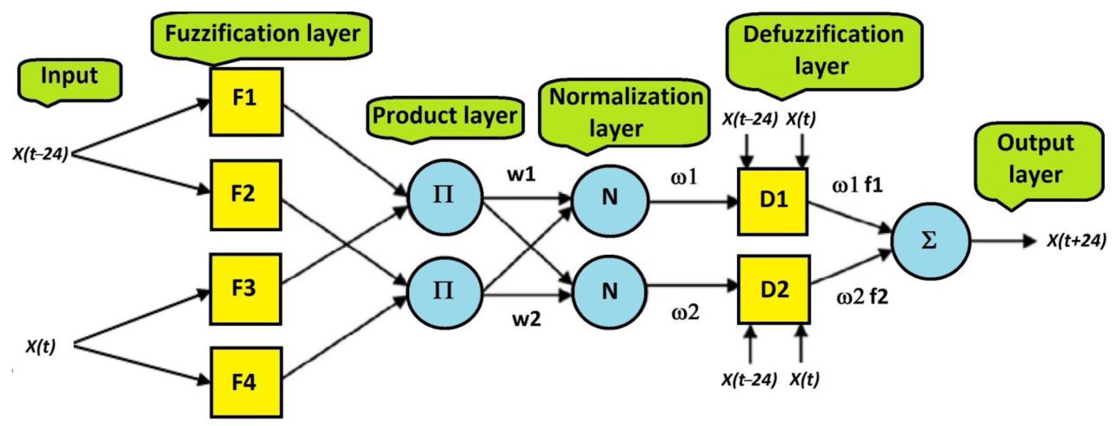Figure 6 presents the architecture of the ANFIS model, described in Section 6, to the prediction of the output variable X(t + 24) taking into consideration two input variables X(t − 24) and X(t). The Figure 7, Figure 8, Figure 9, Figure 10 present the results of estimation and validation of the above forecasting model based on ANFIS. The time series of the output variable X(t + 24), loads on Wednesdays, are characterized by the sinusoidal changeability with the trend (Figure 4). The curve of average temperature on Wednesdays is characterized by similar variability (Figure 5). 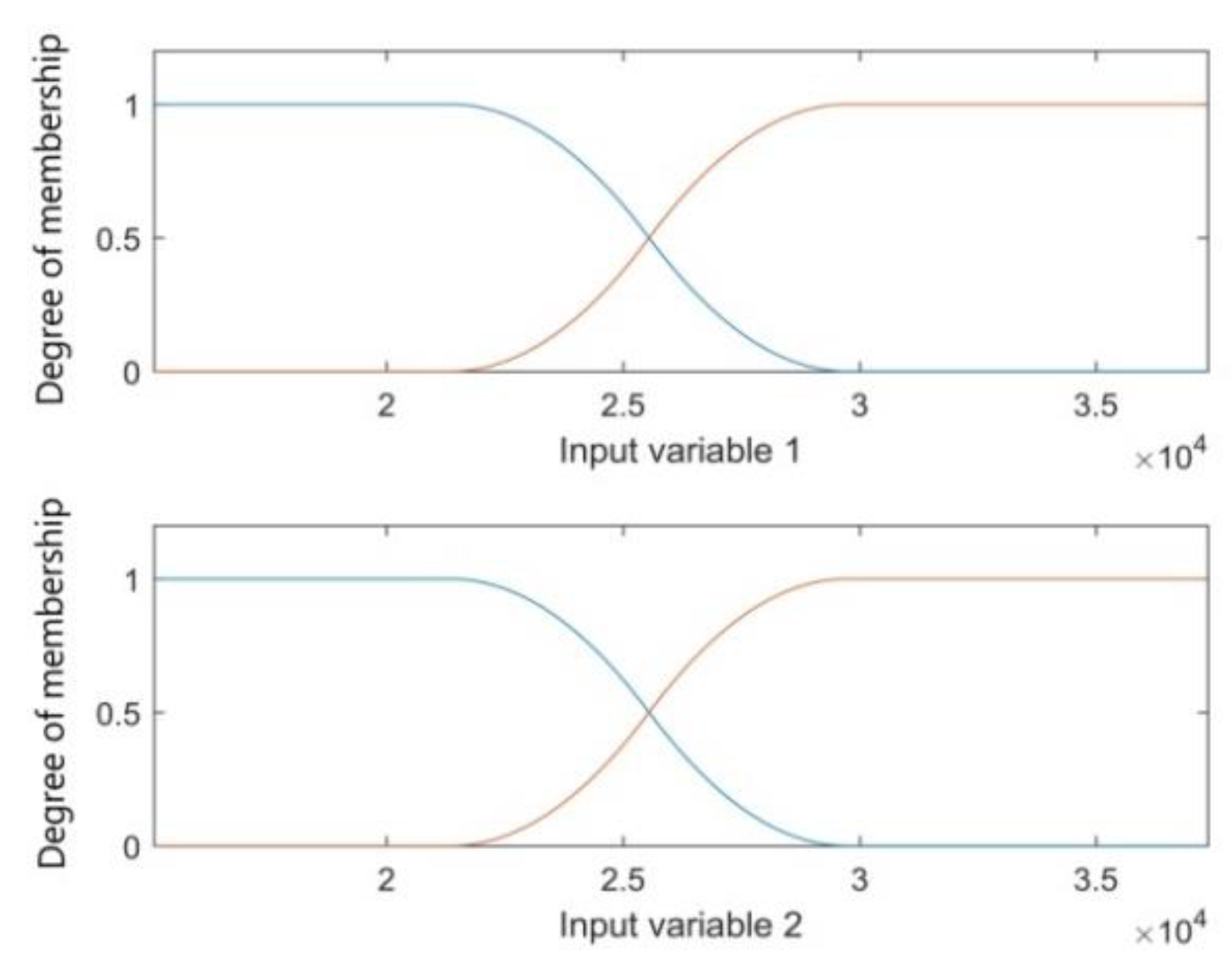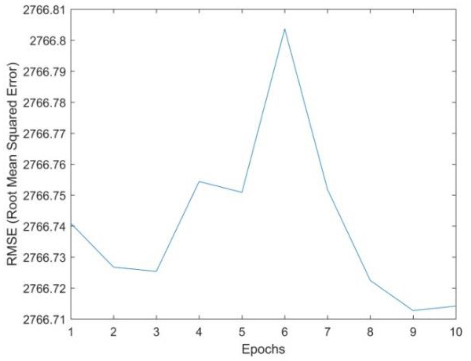Figure 7 presents estimated membership functions w(t). 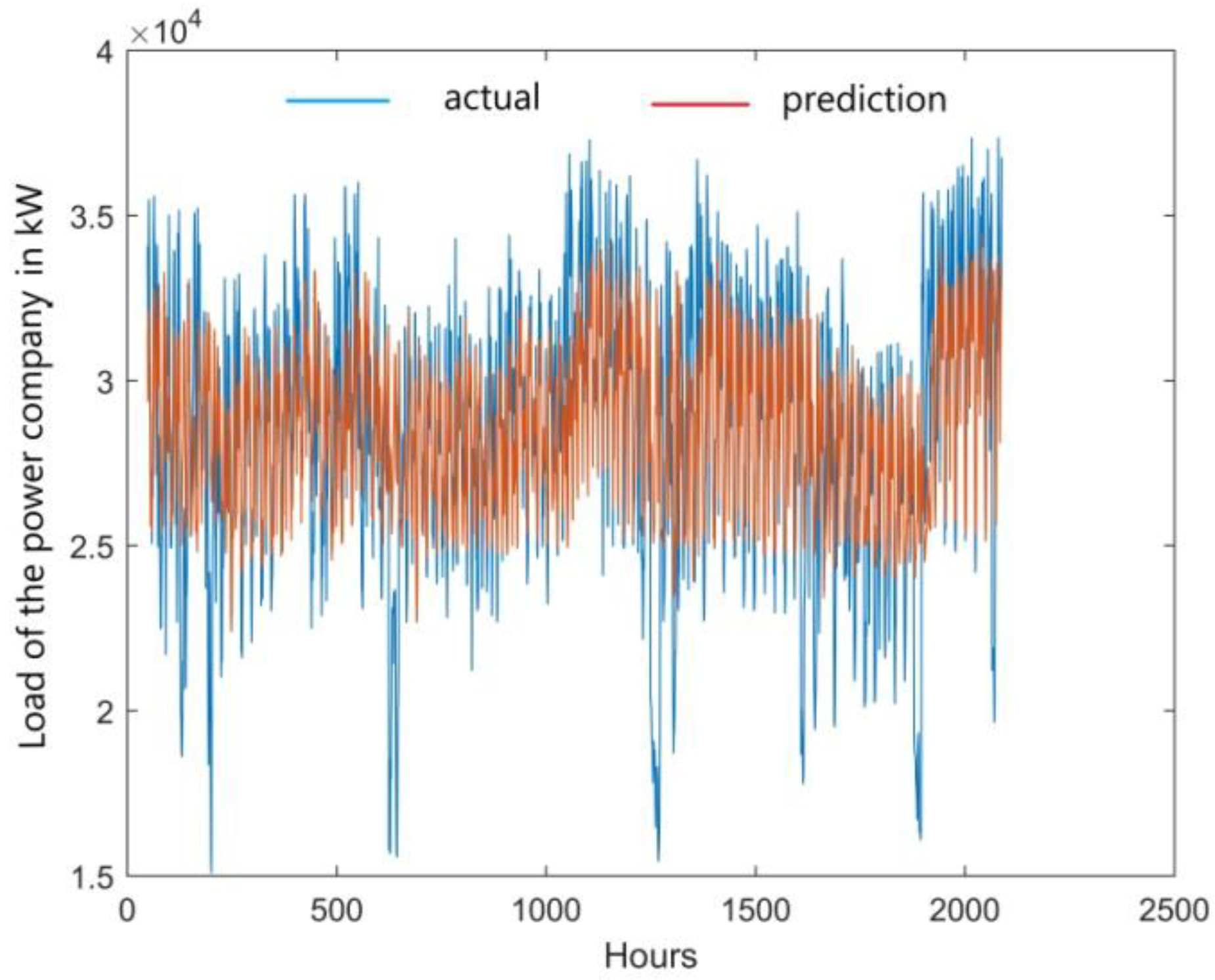Consequently, the RMSE for subsequent epochs in the learning process records a certain decrease (Figure 8). 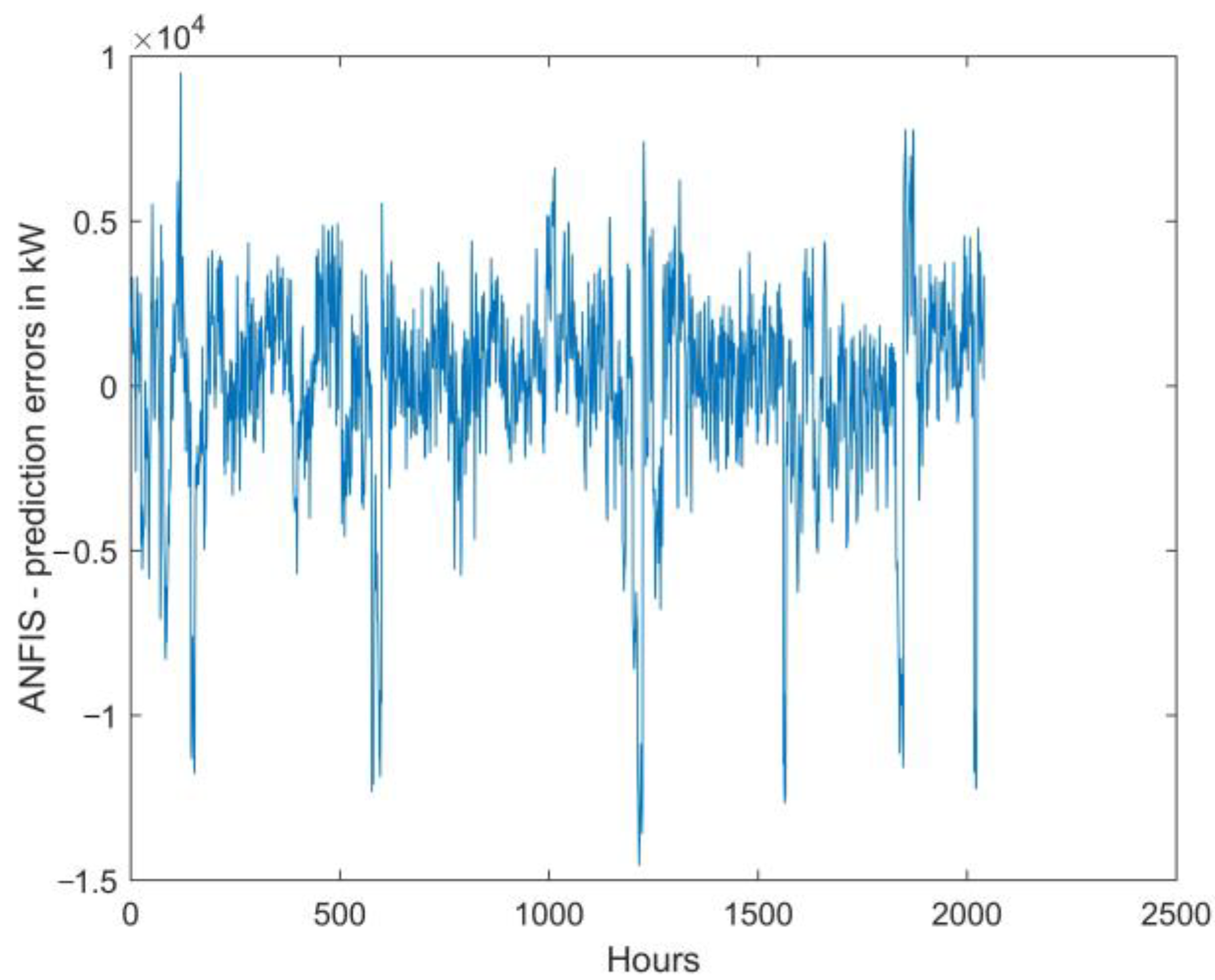The comparison of real data of loads on Wednesdays with the predictions of the ANFIS model (Figure 9) indicates that there are some differences, especially when analyzing values that deviate from the mean profiles, both up and down. Absolute errors of the ex post loads prediction are shown in Figure 10, and MAPE obtained from them is 8.30% (Table 2).

The ANFIS models of load forecast were constructed for each day of the week. Table 2 presents the values of MAPE errors for ex post forecasts of loads in the case of the discussed models.

Some kind of estimation of the ANFIS forecasting models quality is their comparison with the naive model results. For example, in the case of the daily load forecast concerning Wednesday, the naive forecast consists in adopting the relationship of loads from the week preceding the forecast as the forecast proper. Error in case of the naive forecast from the whole set of data, i.e., 2064 observations is MAPE = 9.49%.

Models with the set of variables 5 and 6 for Wednesday characterized by the lowest MAPE errors and at the same time the highest values of integral capacities of information carriers H_m point to the proper selection of exogenous variables.

The results presented in Table 2 confirm the conclusion that adding temperature to the exogenous variables does not improve the accuracy of the forecasting models for the weekdays but improves the accuracy for Sundays when the load is determined by the residential sector. The conclusion concerns the specific Polish power company.

8. Comparison of the Results Presented in Other Publications

Artificial intelligence (genetic algorithms, neural networks and neuro-fuzzy systems) is currently used for forecasting electricity demand and forecasting electrical loads. The models use information in the form of electric, climate and calendar data. The results are usually presented for typical weekdays or holidays. In the case of holidays, relatively different forecasting errors are obtained, as the power load patters of holidays show large differences compared to typical weekdays. Furthermore, the first day of the week (Monday) and the last day (Friday) are characterized by significant deviations from the middle days of the week. This fact justifies the development of forecasting models for a specific day of the week.

The results, presented in many publications [19,26,43,44,46,47,50,51], confirm that the ANFIS model is a reliable forecasting tool. Particularly good results are achieved in the cases of time series with cyclical variability. A mean square error (MSE) below 3% is obtained for different series of power system loads but higher MSE for power company profiles.

The forecast results for the next week of the power system loads, presented in [50], are recognized to be perfect and consistent. A very high accuracy of the ex post forecast was achieved. On the other hand, when using the ANFIS model for medium- or long-term forecasting, the results are usually even better, e.g., the MAPE is equal to 0.4% when monthly electricity demand was forecasted in [51].

It may seem that the results of the ex post forecast accuracy presented in the article are not good because the MAPE is equal to approx. 8–9%. However, the results should be compared with the MAPE equal to approx. 9–11% for the naive forecast, which is always a certain point of reference. The MAPE of the ex post load forecast depends on the nature of the time series of the power company selected for the analysis.

Many publications [4,5,28,50] indicate that the global demand for electricity is influenced by climate variables such as temperature and cloudiness. However, their impact depends on the climate zone. A change in summer temperature in France by one degree causes a change in demand by 500 MW and in winter by about 1450 MW [50]. The power demand changes depend on the use of heating or air-conditioning systems. Climate variables should definitely be applied in medium and long-term forecasting of electricity demand whereas taking them into consideration in the STLF may lead to an imprecise forecast. As shown in the article, the mean daily temperature as the exogenous variable does not improve the accuracy of the ANFIS model for the weekdays. However, the influence of temperature on the load profile on Sundays was observed.

9. Discussion

Recently, a trend to avail of artificial intelligence methods in short-term forecasting has been clearly visible. Using such methods, we lose an opportunity to detect the cause and effect relationships. Most of the machine-type learning algorithms are used as “black-boxes” and the researcher has limited capability to shape the final form of the model. The database and its information capacity, prepared by a researcher, affect usually the final result. Here, the rule garbage in, garbage out (GIGO) is used. Each of the methods adopts one or the whole set of measures of the ex post forecasting model (e.g., Mean Absolute Percentage Error MAPE, Root Mean Square Error RMSE, Mean Absolute Scaled Error MASE, Sum of Squared Errors SSE, Random-Walk Coefficient of Determination R², Root Mean Squared Scaled Error RMSSE, etc.). Note that using different measures generates extremely different forecasts. In general, using the measures of square errors (RMSE, SSE, MSE or R2) and their optimization leads to an optimum forecast being a conditional expected value, the use of MASE and MAE measures model a conditional median and MAPE measures provide a forecast that is difficult to interpret. Artificial intelligence methods are based on the process of learning from pieces of information given in the database. The verification process is performed on a separated part of the database. This procedure undoubtedly provides very good results in ultra short-term forecasts, usually used in the process of controlling various objects. Additionally, in short-term forecasting or even in medium-term forecasting of stable behavior of variables, good results can still be achieved. However, in the case of forecasting technological changes, the results may be unsatisfactory.

The paper shows that the proper selection of the exogenous variables set has an impact on the accuracy of the model. The Hellwig method using integral capacities of information carriers for the selection of an optimum set of exogenous variables is used to construct models reflecting relationships between explaining (exogenous) variables and the explained (endogenous) variable.

The article examines the impact of taking into account an additional exogenous variable—the ambient temperature—on the accuracy of ex post load forecasts. It was demonstrated that for the Polish data adapted for the construction of the ANFIS model, the ambient temperature as an additional input variable does not improve the accuracy of forecasts for the weekdays. The influence of temperature on the load forecasts on Sundays is significant, which confirms the sensitivity of the residential sector loads to temperature changes. It should be however emphasized that this is only a case study for the data of the power subsystem with a load structure with a predominance of the industrial sector. It is difficult to draw general conclusions from a case study, so it makes sense to continue the research for a broad spectrum of data.