Abstract
Many battery state of charge (SOC) estimation methods have been studied for decades; however, it is still difficult to precisely estimate SOC because it is nonlinear and affected by many factors, including the battery state and charge–discharge conditions. The extended Kalman filter (EKF) is generally used for SOC estimation, however its accuracy can decrease owing to the uncertain and inaccurate parameters of battery models and various factors with different time scales affecting the SOC. Herein, a SOC estimation method based on the EKF is proposed to obtain robust accuracy, in which the errors are compensated by a long short-term memory (LSTM) network. The proposed approach trains the errors of the EKF results, and the accurate SOC is estimated by applying calibration values corresponding to the condition of the battery and its load profiles with the help of LSTM. Furthermore, a multi-LSTM structure is implemented, and it adopts the ensemble average to guarantee estimation accuracy. SOC estimation with a root mean square error of less than 1% was found to be close to the actual SOC calculated by coulomb counting. Moreover, once the EKF model was established and the network trained, it was possible to predict the SOC online.
1. Introduction
Recently, owing to global warming, the number of severe natural disasters caused by climate change has increased, and as environmental regulations in each country become very strict, it has become vital to replace internal combustion engine vehicles with other eco-friendly ones, such as electric vehicles (EVs), which constitute the largest proportion of environmentally friendly vehicles in the market today.
Recently, not only EVs but also all types of eco-friendly vehicles, such as hybrid and fuel cell electric vehicles, energy storage system (ESS), and various electronic equipment, have been actively used. For this reason, the importance of a battery management system (BMS) is growing even more.
In a battery management system (BMS), state of charge (SOC) is one of the most important factors for maintaining battery performance and serves as a reference for the BMS to control the battery. Thus, diverse SOC estimation methods have been studied over the last decades.
Research on battery monitoring and energy management of vehicles has been conducted for a long time [1]. Coulomb counting is the most representative method used in battery state estimation [2,3] for which various improvement attempts have been made.
SOC can be expressed by (1), where is the initial state of charge, is the efficiency coefficient () during discharge, and is the battery’s maximum charge. The main advantages of the Coulomb counting method are that it has a simple formula that it is easy to implement. However, it accumulates errors depending on the sensor precision or initial charge state.
Several studies have considered the filter method based on the nonlinear equivalent circuit. Zhihao Yu et al. [4] used the local linearization method on a SOC-open-circuit voltage (OCV) curve and estimated the current SOC based on the Kalman filter; then the extended Kalman filter (EKF) and adaptive EKF (AEKF) were applied to improve the Thevenin model to determine the battery charge state [5]. Further, another study used a dual-time scale estimator by employing the EKF to estimate the SOC of each cell based on the SOC of the entire battery pack [6], and a hardware-in-the-loop test of the second-order equivalent circuit model with the EKF [7] was conducted. Apart from the EKF, for accurate SOC measurements, parameter estimation through an H-infinity filter is usually performed to reflect the battery characteristics under different operating conditions in real-time, and the SOC is estimated using the unscented Kalman filter (UKF) based on this parameter value [8]. However, as shown in [9], the equivalent circuit models representing Li-Ion batteries vary, thus that the filtering methods have different state equations for each equivalent model. This means that the results of the filtering method depend considerably on the type and accuracy of the model. In addition to these methods, the method of recursive least square (RLS) used to predict the dynamic behavior of the battery in a hybrid electric vehicle (HEV) [10] or electric vehicle (EV) [11] also highly depend on the type and accuracy of the model used.
Because the state of health (SOH) is also a very important factor for BMS, it has attracted the interest of many researchers. There have been studies such as developing reliable and accurate models to measure SOC and SOH online at the same time [12]. However, owing to the limitations of the model-based methods described earlier, the mainstream of the SOC and SOH estimation studies is to add learning-based (data-based) methods or replace existing model-based methods. The genetic learning algorithm is also utilized to estimate SOC. In the first step, the fuzzy c-means method is used to cluster the sampled training data in the driving cycle (as with a Federal Urban Driving Schedule(FUDS)-based test), and these results are then fed to a topology and antecedent parameter-learning algorithm with an R-LSM. In the second step, a backpropagation learning algorithm is executed to optimize the antecedent and consequent parameters [13]. The authors of [14] developed a synthesis method to estimate SOH and remaining useful life (RUL) using an advanced filter and artificial neural network (ANN), while [15] a data-driven method is applied to identify the parameters of the model to obtain the open-circuit voltage (OCV). There are also many studies that utilize support vector machine (SVM), such as using a partial charging curve with SVM for SOH estimation [16] or using a least square support vector machine (LS-SVM) [17]. The technique proposed in [18] aims to predict the SOC of high-capacity lithium iron manganese phosphate ( battery cells from experimental datasets using SVM. In addition, in [19], aiming to improve the model performance of battery models, a sparse least square SVM (LS-SVM) model was built, and it utilized an UKF to estimate the SOC based on a sparse LS-SVM battery dynamic model.
Further, the recurrent neural network (RNN) has been frequently utilized in many studies, including battery management systems. RNN’s ability to analyze time series data has already been utilized in various fields such as language modeling [20], driving assistance system [21], and human eye fixation tracking [22]. In particular, RNNs are also widely used in fuel cells that have electrochemical characteristics similar to those of batteries. Reference [23] proposed a time series fault diagnosis method based on the bidirectional long short-term memory (Bi-LSTM) for polymer electrolyte membrane fuel cell (PEMFC). This study used the Bi-LSTM with t-distributed stochastic neighbor embedding (t-SNE) to decrease the dimensionality of normalized data to the intrinsic dimensionality to extract key characteristic variables.
Similar to the fault diagnosis of fuel cells, the SOC and SOH estimation of batteries is not a one-step process but a multivariable time series process, and it is more in line with the physical evolution law of electrochemical systems. Therefore, many studies use RNNs for battery SOC estimation. In addition to the most basic form of the vanilla RNN, LSTM can be applied to estimate SOC [24], a convolutional neural network can be added to the LSTM [25], or a modified one such as the gated recurrent network can be used to estimate the SOC of lithium-ion batteries [26].
To take advantage of both the filtering method and the data-driven method, this study uses the method of error compensation through an LSTM after estimating the primary SOC using the EKF instead of directly predicting the SOC using a neural network. In addition, this novel method improves the estimation accuracy using a sort of ensemble average after estimating the SOC through multiple LSTM structures to reflect various phenomena with their own cycle or period on the time scale.
The contributions of the proposed novel method in this paper are summarized as follows.
- (1)
- Despite the use of the SOC–OCV model for estimating the SOC state, this novel method can estimate the accurate OCV and SOC right after battery discharge without any rest period to observe the OCV.
- (2)
- It is possible to reduce the influence of the model parameter uncertainty and the SOC–OCV model error, which has a profound effect on the SOC estimation in existing model-based methods.
- (3)
- Using multiple LSTM network structures and a sort of ensemble average, phenomena occurring over a relatively long period of time (e.g., aging, non-homogeneity in the electrochemical state between cells) as well as phenomena occurring immediately (e.g., changes in temperature) can be reflected in the SOC estimation.
This paper is divided into six sections. Section 2 introduces the mathematical model of the used battery and the state equation for the filter method. The proposed SOC estimation methods are described in Section 3. In Section 4, the experimental environments are presented, and the results and discussion are stated in Section 5. Finally, the conclusions of this study are given in Section 6.
2. Modeling Battery Dynamics
2.1. Identification of Equivalent Circuit Parameters
In this study, the first-order circuit was selected as a model to minimize complexity and computational burden. As the errors caused by model uncertainty will be offset by the LSTM, an increase in the computational burden using more complex models will become unnecessary.
The first-order R-C circuit, shown in Figure 1, comprises an internal resistance , a polarization resistance , and a polarization capacitance . is the open-circuit voltage, is the terminal voltage, and is the polarization voltage for and , which represents the transient response due to polarization. In general, the model parameters are changed by various factors, such as the discharge or charge profiles, SOC state, temperature, and aging state, and these changes increase the model parameter error unless the model parameters are accurately evaluated. However, in this study, monitoring or estimating the internal circuit elements in real-time for accurate prediction is not needed because these errors are compensated by the RNN-LSTM neural network.
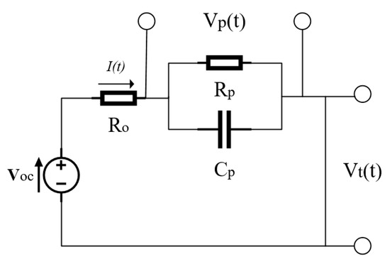
Figure 1.
Schematic of the first-order R-C circuit model.
Instead, in this paper, only one parameter identification was performed for each experiment. Finally, the average value of the estimated parameters from all the trials was used for the EKF. In [27], the step response analysis (SRA) was used to estimate the internal parameters of the first-order equivalent model.
By substituting (3) into (2) and separating and on both sides,
By applying the Laplace transform to (4),
where , and imply t = 0 before any external perturbation to the system.
Here, the inverse Laplace transform is applied to observe the behavior of .
- The first term on the right side of (6):
- The second term on the right side of (6):If (8) can be expressed as
- The third term on the right side of (6):and . can be determined as illustrated below.
Finally, can be calculated from the time constant () of the battery response that occurs when a current change is applied.
From (12)–(14) and the unit-step current experiment of the battery system, all the battery model elements used in this study can be illustrated as in Table 3.
2.2. State Equation for the Battery Model
Assuming that the battery is a large capacitor of capacitance , the state equation can be obtained by solving the differential equations given below.
where is the amount of charge stored in . The complete solution of (16) can be obtained by obtaining solutions for each of the two cases below.
- Complementary solution:
- Particular solution:In the steady state, is assumed to be a current value.
After obtaining A using the initial conditions, the complete solution to (16) is as shown below.
However, (22) only shows the zero-state response because the initial time and initial value are assumed to be zero. To complete the response of the first-order RC circuit, a zero-input response is added, and discretization is performed to apply the filtering method.
By combining (15) and (23), the state equation with the state vector composed of the open-circuit voltage and the polarization voltage can be constructed as given by (24) and (25).
3. EKF–LSTM-Based SOC Estimation Method
3.1. Extended Kalman Filter and SOC–OCV Estimation
Based on the state equation of the equivalent circuit obtained in the previous section, OCV estimation using the Kalman filter is performed. In this study, SOC is estimated using the SOC–OCV relation after first estimating the OCV through the filter. The nonlinear system is usually modeled as in (26–27).
where is the state transition function, is the measurement function, is the process noise, and is the measurement noise. and are the white Gaussian stochastic processes with zero mean. Furthermore, the covariance matrices and . Like the linear Kalman filter (LKF), the EKF is performed in two parts: Prediction and update. The most important difference between LKF and EKF is the linear approximation, which is performed by applying the Taylor series to the nonlinear functions and to obtain a Jacobian matrix. EKF only uses the first-order approximation.
Kalman Filter for Estimation.
| (i) Prediction process | |
| (31) | |
| (32) | |
| (ii) Update process | |
| (33) | |
| (34) | |
| (35) | |
As mentioned earlier, the calculated OCV using the EKF can be converted into the SOC through the SOC–OCV function. In this study, (36) is obtained by curve fitting using the obtained results from the experimental data, and the used coefficients are calculated in Table 1.

Table 1.
5th order state of charge–open-circuit voltage (SOC–OCV) Relation Function Coefficient Values.
In general, when estimating the OCV or SOC using a filter, fitting an accurate SOC–OCV relationship is as important as precisely estimating the model parameters. Even when OCV is very accurately estimated, if the relationship with SOC is not correctly established, there will be a large error in the SOC dimension. Therefore, many studies focus on establishing an accurate relationship by accurately fitting the SOC–OCV relationship based on experimental data [4] or by performing linearization using various methods, such as the cubic Hermite method [28].
In this study, data fitting was performed using polynomials of various orders to obtain the relationship as accurately as possible. However, even if the approximation by curve fitting differs from the actual SOC–OCV function, the error will be compensated by the LSTM network used in this study.
3.2. LSTM
Unlike other artificial neural networks, RNN has a recursive form in which the output data are used as input to the next stage. Because of these characteristics, the RNN structure can be expressed in a form in which each RNN cell is continuously attached with time, as shown in Figure 2. In addition, the user can determine the sequence lengths according to this characteristic of the RNN structure thus that the network can be trained for many factors that affect the battery system with various time scales. As previously stated, the battery dynamic behavior is not a single-step process, thus using an RNN can yield better results than using other artificial neural networks.
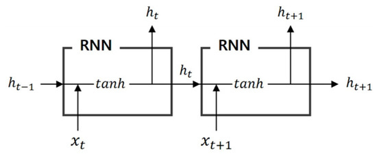
Figure 2.
Structure of the recurrent neural network.
The hidden state is expressed by (37), where W and U are the weights of the input and the hidden state of the previous time , respectively, b is the bias, and is the nonlinear function (here, is a hyperbolic tangent). As the RNN progresses, a long-term dependency problem occurs owing to the gradient vanishing caused by the used nonlinear function. Therefore, the LSTM artificial neural network was designed and used in this study.
LSTM is an artificial neural network based on RNN, and it solves the long-term dependency problem using not only the hidden state but also the cell state as the input of the next time-step as shown in Figure 3. In the LSTM, the forget gate determines how much of the cell state from the previous time-step is reflected at the current time t. As the value passed through, the sigmoid function approaches 1, implying that the previous cell state is more reflected. The input gate is used to set the degree of the effect on the output of the current input, and it is represented by the Hadamard product of and . Here, because uses the hyperbolic tangent as an activation function, it has a value between −1 and 1. The equations related to the LSTM are given by (38)–(44), including the equations for , and , which are the outputs of the LSTM cell. In this paper, the study was conducted using the LSTM network of the two-layer architecture shown in Figure 4.
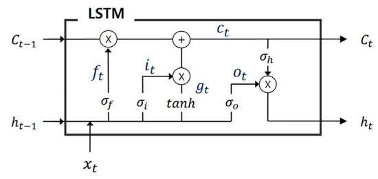
Figure 3.
Internal structure of the single long short-term memory (LSTM) cell.
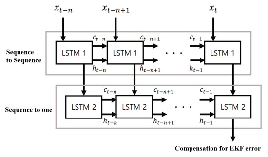
Figure 4.
Architecture of the proposed two-layer LSTM network.
Long Short-Term Memory Calculation.
| LSTM Calculation | |
| (38) | |
| (39) | |
| (40) | |
| (41) | |
| (42) | |
| (43) | |
| (44) | |
3.3. EKF–LSTM Method
The biggest problem in applying the estimation method using the OCV–SOC relation to real applications is that it requires a very long rest period to measure the OCV owing to the characteristics of the lithium-ion battery. Therefore, to design a method for estimating precise OCV values by using only the data up to right after the discharge, this paper proposes an EKF–LSTM coupling method. This is expected to compensate for the nonlinear battery behavior that is not predictable by EKF and for the effects of the various factors that are not even expressed in the dynamics but affect the actual OCV, such as aging or non-homogeneity.
However, it is impossible to reflect the various factors that affect the battery dynamic behavior with their own time scales within one LSTM network. For example, having different time scales means that each of the factors affecting the battery behavior works with its own time length and respective time point. Thus, multiple networks with various LSTM cell numbers are required. Accordingly, in this study, we designed multiple LSTM structures and took a sort of ensemble average of them as network estimation results to compensate for the EKF results. The entire process used in the study is shown in Figure 5.
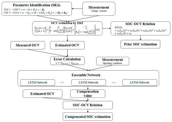
Figure 5.
Process of the EKF with the multi-LSTM-based OCV and SOC estimation.
4. Experiment
4.1. System Configuration
In the experiment, a Beckhoff IPC-C6920 PC and an Anybus CAN communicator were used, and the PC and BMS exchanged data through CAN and EtherCAT networks as shown in Figure 6. The DC load was connected to the PC via RS-232 serial communication to receive the current loading profile of the battery. In the battery pack, 10 slave BMSs and 1 master BMS measured the voltage, current, and temperature. Each slave BMS measured the battery pack status every 10 ms, and the master BMS transmitted data to the IPC-C6920 once every 100 ms. The performance of the used battery pack in the experiment is presented in Table 2.
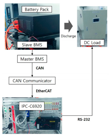
Figure 6.
Battery system and communication diagram.
Table 2.
Specification of the Battery Pack.
4.2. Parameter Identification
The SOC estimation that only used the model-based method was considerably influenced by the accuracy of the model parameters, which vary depending on the current load profile, SOC state, aging status, temperature, etc. Therefore, accurate parameter estimation in real time was required for precise SOC estimation. Usually, in many application fields, the least squares method or the filter method is used for electric circuit model (ECM) parameters; however, this results in an increase in the system’s complexity and computational burden. In this study, it was assumed that the model errors caused by the changes in the model parameters during operation can be sufficiently compensated without estimating these parameters in real time using EKF and LSTM together.
Therefore, in this experiment, model parameter estimation was performed just once in the initial state of each discharge. Then, SOC estimation was performed using only EKF and LSTM. In addition, the required data diversity for network learning was secured through 8 different current load profiles as shown in Figure 7. Accordingly, it was confirmed that the proposed method could accurately estimate SOC without real-time model parameter monitoring; Table 3 shows the estimated average model parameter values according to (12)–(14).
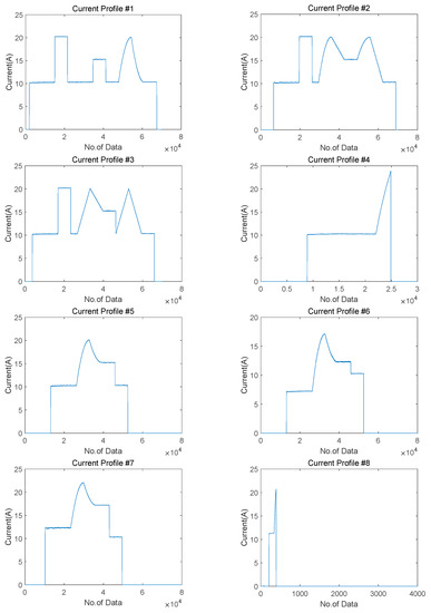
Figure 7.
Current load profiles used in the experiment.
Table 3.
Values of the model parameters constituting the first-order RC model.
When parameter estimation was performed using SRA by setting a higher data sampling frequency, more accurate values could be obtained as the system response at was required for calculating , as shown in (7). However, as the sampling frequency increased, the memory burden exponentially increased. The method proposed in this paper aimed at reducing the sensitivity of the model parameters to the estimation results, thus we applied a relatively low sampling frequency of 1 kHz in the experiment.
4.3. Data Acquisition
Using the current load profile shown in Figure 7, the discharge and data acquisition were performed. The experiment was conducted in a range of less than 75% of the initial SOC of the battery, which was discharged to 65%. To check the actual OCV of the battery pack after the discharge for comparison with the results predicted by the proposed method, all the voltage values were recorded during a rest period of 3 h after the discharge with a sampling frequency of 100 Hz.
5. Results and Analysis
5.1. SOC Estimation Using EKF Only
First, the OCV estimation was performed by using only EKF with nine sets of data, which were obtained through experiments. Then, the estimated OCV was substituted into (36) to obtain the SOC of the battery pack.
The root mean square error (RMSE) values of the nine experiments are presented in Table 4, and as seen in the table, the RMSE values of OCV and SOC were up to 3.0 V and 8.0%, respectively.
Table 4.
Root mean square error (RMSE) values of SOC and OCV estimated using only EKF.
5.2. SOC Estimation Using EKF and Single LSTM
After predicting SOC using EKF, a single LSTM layer was used to compensate for the error between the real and estimated OCVs using EKF. To select a single LSTM for compensating the error of EKF, 50 different LSTM networks were created to evaluate their error estimation performance. Among the 50 networks, a network that performed an extremely accurate estimation of the actual OCV of Experiment 1 was selected as the representative single LSTM network to compensate for the EKF estimation results. The selected network had a difference of 0.0 V in the OCV estimation for Experiment 1, while other networks had an average difference of 0.3 V for the same experiment. As observed in Table 5, the sum and average of the OCV and SOC RMSE for Experiments 1–9 were greatly improved by just applying a single LSTM to the EKF results.
Table 5.
RMSE values of SOC and OCV estimated using the single LSTM network.
5.3. SOC Estimation Using EKF and Multi-LSTM Network
To reflect factors with various time scales in the estimation results, a structure using a sort of ensemble average of the multi-LSTM networks was implemented. To prove that the multi-LSTM structures with various numbers of cells can reflect factors with various time scales in the results, 50 networks with an identical network structure and hyper-parameters except for the sequence length were created. Among them, 10 networks were selected based on the sum of the errors of all the experiments’ data. As mentioned before, since the network that outputted the most outstanding estimation result for Experiment 1 out of the 50 networks was used for the single LSTM, even if the ensemble average of the multi-LSTM network were used, the estimation error of Experiment 1 would be naturally greater than that of the single LSTM. However, what this study aims to confirm is that using multi-LSTM leads to a reduction in the sum and average of errors of all the experiments’ data. If the intended result is confirmed, then not only is the method more suitable for estimating the OCV and SOC of the lithium-ion battery but it can also avoid overfitting to specific experiment data. The estimated results of this method are shown in Table 6.
Table 6.
RMSE of SOC and OCV Estimated Using the Ensemble Network.
To more clearly show the results, the estimation results and errors for each method used in this study are plotted in Figure 8. The graphs on the left side show OCV, and the ones on the right side represent the SOC predicted using EKF, EKF with the single LSTM, and EKF with multi-LSTM.
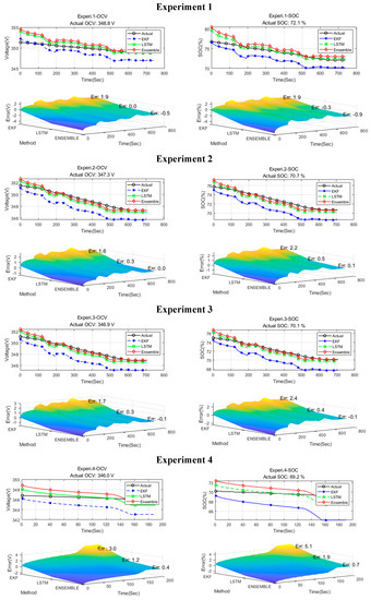
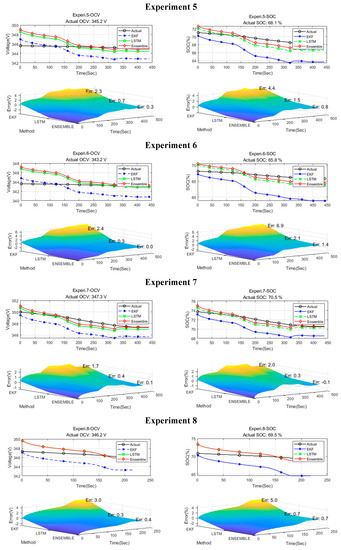
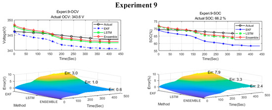
Figure 8.
OCV and SOC estimated using EKF, EKF with single LSTM, and EKF with multi-LSTM networks (ensemble averages).
In Figure 8, the behavior up to 100 s after the discharge is over is expressed, and the corresponding part is shown as a flat area in the graph.
However, our proposed method performs OCV estimation immediately after discharging (just before flat region) without any rest period.
5.4. Results
First, the estimated OCV was obtained by applying the battery model and the model parameters obtained using SRA to EKF. The OCV of the battery predicted using EKF had a difference of at least 1.6 V to a maximum of 3.0 V for each experimental data, and the sum and average of the errors were 20.4 V and 2.3 V, respectively. When SOC was calculated by substituting the obtained OCV into (36), SOC errors in the range of 1.9–8.0%, a sum of SOC errors of 38.0%, and an average of errors of 4.2% were confirmed as the results.
Once the difference between the estimation results obtained using EKF and the actual OCV is calculated, it can be used as an input to the LSTM with the current and voltage data measured during discharge. This network can predict the error that the EKF estimation would have according to the battery behavior, the past operating conditions, and the current battery condition. Then, this result is applied as a compensation value to the prior OCV prediction by EKF. When the corrected OCV is obtained by compensation, it is possible to estimate the improved SOC by inputting it into the OCV–SOC relation.
Table 5 gives the error compensation results when a single LSTM network is used. By applying a single LSTM to the entire experiments data, the average of errors of OCV was 4.5 times less compared with using EKF alone. When SOC was calculated using the corrected OCV, the sum of errors of SOC was reduced from 38.0% to 11.0%, and the average of errors also exhibited a significant reduction from 4.2% to 1.2%.
Although the results of using a single LSTM are significantly better than those of using EKF alone, it cannot be said that this structure effectively reflects various factors with different time scales because it only uses a single LSTM structure with one predefined sequence length.
To obtain better results by reflecting various factors with different time scales, 10 networks with the best performance based on the sum of errors of OCV among the 50 networks were selected for the multi-LSTM network and ensemble averages. After using the multi-LSTM and ensemble averages, the OCV estimation error of the entire data converged between 0.0 V and 0.7 V, the OCV sum of errors became 2.2 V, and the average of errors became 0.2 V, which is approximately two times more accurate than using EKF with a single LSTM. Considering the results in terms of SOC, the sum of errors of SOC decreased to 7.3%, and the average of errors decreased from 1.2% to 0.8%, showing an accuracy improvement of 33.3% compared to the results of EKF with a single LSTM. The comprehensive results of this paper are detailed in Table 7 as follows.
Table 7.
Comparison of errors according to each estimation method.
6. Conclusions
This paper introduces a new OCV and SOC estimation method for lithium-ion batteries that is based on the compensation of the EKF errors using multi-LSTM networks with ensemble averages. In this study, the proposed method used EKF to estimate the OCV and SOC values using a battery model and model parameters calculated from SRA. Afterward, the errors between the actual and estimated values using EKF were entered into the LSTM network with the current and voltage data measured during the discharge to generate the compensation value for accurate OCV and SOC estimation.
In the experiment, when SOC was calculated by EKF only, SOC errors in the range of 1.9–8.0%, a sum of SOC errors of 38.0%, and an average of errors of 4.2% were confirmed as results. By applying a single LSTM to the entire experiments data, the average of errors of OCV was 4.5 times less compared with using EKF alone. The sum of errors of SOC was reduced from 38.0% to 11.0%, and the average of errors also exhibited a significant reduction from 4.2% to 1.2%.
After using the multi-LSTM and ensemble averages, the sum of errors of SOC decreased to 7.3%, and the average of errors decreased from 1.2% to 0.8%, showing an accuracy improvement of 33.3% compared to the results of EKF with a single LSTM.
By using EKF and LSTM together, it was possible to estimate the state of the battery from the standpoint of “Physical-Information”, and the multi-LSTM networks could also estimate OCV and SOC reflecting the effects of many factors affecting the battery dynamics with their own time scales. In addition, as the error compensation method that uses a multi-LSTM structure and a sort of ensemble average has a certain regularization effect to prevent overfitting, the proposed method is very effective in estimating the state of the OCV and SOC.
Finally, the method proposed in this paper is suitable for practical applications because it can accurately estimate the OCV immediately after discharging is over without having to wait for a rest period, which is usually required for perfect OCV measurements in the existing method, as shown in Figure 9.
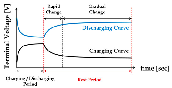
Figure 9.
Terminal voltage change in the rest period [3].
Author Contributions
Conceptualization, D.S. and S.Y.; methodology, D.S.; software, B.Y.; validation, D.S. and B.Y.; formal analysis, S.Y.; investigation, D.S.; writing—original draft preparation, D.S.; writing—review and editing, D.S. and S.Y.; visualization, B.Y.; supervision, S.Y.; All authors have read and agreed to the published version of the manuscript.
Funding
This research received no external funding.
Institutional Review Board Statement
Not applicable.
Informed Consent Statement
Not applicable.
Data Availability Statement
Not applicable.
Conflicts of Interest
The authors declare no conflict of interest.
References
- Meissner, E.; Richter, G. Battery monitoring and electrical energy management. J. Power Sources 2003, 116, 79–98. [Google Scholar] [CrossRef]
- Ng, K.S.; Moo, C.; Chen, Y.; Hsieh, Y. Enhanced coulomb counting method for estimating state-of-charge and state-of-health of lithium-ion batteries. Appl. Energy 2009, 86, 1506–1511. [Google Scholar] [CrossRef]
- Jeong, Y.M. Enhanced coulomb counting method with adaptive SOC reset time for estimating OCV. In IEEE Energy Conversion Congress and Exposition ECCE, Proceedings of the 2014 Energy Conversion Congress and Exposition, Pittsburgh, PA, USA, 14–18 September 2014; IEEE: New York, NY, USA, 2014; pp. 4313–4318. [Google Scholar]
- Yu, Z.; Huai, R.; Xiao, L. State-of-charge estimation for lithium-ion batteries using a Kalman filter based on local linearization. Energies 2015, 8, 7854–7873. [Google Scholar] [CrossRef]
- He, H. State-of-charge estimation of the lithium-ion battery using an adaptive extended Kalman filter based on an improved Thevenin model. IEEE Trans. Veh. Technol. 2011, 60, 1461–1469. [Google Scholar]
- Dai, H.; Wei, X.; Sun, Z.; Wang, J.; Gu, W. Online cell SOC estimation of Li-ion battery packs using a dual time-scale Kalman filtering for EV applications. Appl. Energy 2012, 95, 227–237. [Google Scholar] [CrossRef]
- Chen, Z.; Fu, Y.; Mi, C.C. State of charge estimation of lithium-ion batteries in electric drive vehicles using extended Kalman filtering. IEEE Trans. Veh. Technol 2013, 62, 1020–1030. [Google Scholar] [CrossRef]
- Yu, Q.; Xiong, R.; Lin, C.; Shen, W.; Deng, J. Lithium-ion battery parameters and state-of-charge joint estimation based on H-infinity and unscented Kalman filters. IEEE Trans. Veh. Technol. 2017, 66, 8693–8701. [Google Scholar] [CrossRef]
- Hu, X.; Li, S.; Peng, H. A comparative study of equivalent circuit models for Li-ion batteries. J. Power Sources 2012, 198, 359–367. [Google Scholar] [CrossRef]
- Kim, H. Modeling and characteristic analysis of HEV Li-ion battery using recursive least square estimation. Trans. KASE 2009, 17, 130–136. [Google Scholar]
- He, H.; Zhang, X.; Xiong, R.; Xu, Y.; Guo, H. Online model-based estimation of state-of-charge and open-circuit voltage of lithium-ion batteries in electric vehicles. Energy 2012, 39, 310–318. [Google Scholar] [CrossRef]
- Huang, S.; Tseng, K.; Liang, J.; Chang, C.; Pecht, M. An online SOC and SOH estimation model for lithium-ion batteries. Energies 2017, 10, 512. [Google Scholar] [CrossRef]
- Hu, X.; Li, S.E.; Yang, Y. Advanced machine learning approach for lithium-ion battery state estimation in electric vehicles. IEEE Trans. Transp. Electrific. 2016, 2, 140–149. [Google Scholar] [CrossRef]
- Zhang, S.; Zhai, B.; Guo, X.; Wang, K.; Peng, N.; Zhang, X. Synchronous estimation of state of health and remaining useful lifetime for lithium-ion battery using the incremental capacity and artificial neural networks. J. Energy Storage 2019, 26, 100951. [Google Scholar] [CrossRef]
- Ma, Z.; Yang, R.; Wang, Z. A novel data-model fusion state-of-health estimation approach for lithium-ion batteries. Appl. Energy 2019, 237, 836–847. [Google Scholar] [CrossRef]
- Feng, X.; Weng, C.; He, X.; Han, X.; Lu, L.; Ren, D.; Ouyang, M. Online state-of-health estimation for Li-Ion battery using partial charging segment based on support vector machine. IEEE Trans. Veh. Technol 2019, 68, 8583–8592. [Google Scholar] [CrossRef]
- Deng, Y.; Ying, H.; Jiaqiang, E.; Zhu, H.; Wei, K.; Chen, J.; Zhang, F.; Liao, G. Feature parameter extraction and intelligent estimation of the State-of-Health of lithium-ion batteries. Energy 2019, 176, 91–102. [Google Scholar] [CrossRef]
- Antón, J.C.Á. Support vector machines used to estimate the battery state of charge. IEEE Trans. Power Electron. 2013, 28, 5919–5926. [Google Scholar] [CrossRef]
- Zhang, L.; Li, K.; Du, D.; Zhu, C.; Zheng, M. A sparse least squares support vector machine used for SOC estimation of Li-ion Batteries. IFAC PapersOnLine 2019, 52, 256–261. [Google Scholar] [CrossRef]
- Sundermeyer, M. LSTM neural networks for language modeling. In Proceedings of the 13th Annual Conference of the International Speech Communication Association, Portland, OR, USA, 9–13 September 2012; pp. 194–197. [Google Scholar]
- Kim, H.; Park, S. LSTM based LKAS yaw rate prediction model using lane information and steering angle. Trans. KSAE 2018, 26, 279–287. [Google Scholar] [CrossRef]
- Cornia, M.; Baraldi, L.; Serra, G.; Cucchiara, R. Predicting human eye fixations via an LSTM-based saliency attentive model. IEEE Trans. Image Process. 2018, 27, 5142–5154. [Google Scholar] [CrossRef]
- Liu, J.; Li, Q.; Yang, H.; Han, Y.; Jiang, S.; Chen, W. Sequence fault diagnosis for PEMFC water management subsystem using deep learning with t-SNE. IEEE Access 2019, 7, 92009–92019. [Google Scholar] [CrossRef]
- Yang, F.; Li, W.; Li, C.; Miao, Q. State-of-charge estimation of lithium-ion batteries based on gated recurrent neural network. Energy 2019, 175, 66–75. [Google Scholar] [CrossRef]
- Song, X.; Yang, F.; Wang, D.; Tsui, K. Combined CNN-LSTM Network for State-of-charge estimation of lithium-ion batteries. IEEE Access 2019, 7, 88894–88902. [Google Scholar] [CrossRef]
- Abbas, G. Performance comparison of NARX&RNN-LSTM neural networks for LiFePO4 battery state of charge estimation. In Proceedings of the 2019 16th International Bhurban Conference on Applied Sciences and Technology IBCAST, Islamabad, Pakistan, 8–12 January 2019; pp. 463–468. [Google Scholar]
- Shin, D.H. Real time water contents measurement based on step response for PEM fuel cell. IJPEM Green Technol. 2019, 6, 883–892. [Google Scholar] [CrossRef]
- Ko, Y. SOC and SOH estimation method for the lithium batteries using single extended Kalman filter. In Proceedings of the KIPE General Meeting andAutumn Conference, Seoul, Korea, 22 November 2019; pp. 79–81. [Google Scholar]
Publisher’s Note: MDPI stays neutral with regard to jurisdictional claims in published maps and institutional affiliations. |
© 2021 by the authors. Licensee MDPI, Basel, Switzerland. This article is an open access article distributed under the terms and conditions of the Creative Commons Attribution (CC BY) license (http://creativecommons.org/licenses/by/4.0/).