Abstract
Traffic congestion is becoming a critical problem in urban traffic planning. Intelligent transportation systems can help expand the capacity of urban roads to alleviate traffic congestion. As a key concept in intelligent transportation systems, urban traffic networks, especially dynamic traffic networks, can serve as potential solutions for traffic congestion, based on the complex network theory. In this paper, we build a traffic flow network model to investigate traffic congestion problems through taxi GPS trajectories. Moreover, to verify the effectiveness of the traffic flow network, an actual case of identifying the congestion areas is considered. The results indicate that the traffic flow network is reliable. Finally, several key problems related to traffic flow networks are discussed. The proposed traffic flow network can provide a methodological reference for traffic planning, especially to solve traffic congestion problems.
1. Introduction
Traffic congestion is a major problem in traffic planning. With the rapid increase in the number of motor vehicles in cities, the problems caused by traffic congestion are becoming increasingly critical. Several researchers have attempted to solve traffic congestion problems by applying intelligent transportation systems [,]. In this regard, although intelligent transportation systems cannot fundamentally solve the problem of traffic congestion, they can enhance the traffic efficiency and capacity of the roads through the identification and enhancement of unreasonable traffic modes. Thus, intelligent transportation systems may represent an effective solution to alleviate traffic congestion and facilitate decision making in traffic planning [,,].
As a key part of intelligent transportation systems, urban traffic networks can help examine traffic congestion problems because the congestion status of urban roads is closely related to the urban traffic network []. Generally, an urban traffic network can be divided into the urban static and dynamic traffic networks [,,] based on the topological structure of the urban roads and actual traffic flow. Moreover, both the static and dynamic networks exhibit the characteristics of complex networks [,]. Thus, certain methods pertaining to complex networks can be applied to urban traffic networks to analyze the problems caused by traffic congestion [,]. When investigating traffic congestion problems based on the complex network theory, a key task is to build an urban traffic network. As mentioned previously, an urban traffic network includes an urban static and dynamic traffic network. Usually, the urban static traffic network can be obtained as follows—the nodes are the intersections of the urban roads, and the edges are the roads between the intersections. Generally, most traffic congestion events occur at the intersections (nodes) due to the large traffic flow. A higher traffic flow at a node corresponds to a higher possibility of the node being congested. However, the urban static traffic network is built based on the topological structure of the urban roads and thus cannot reflect the traffic flow []. For example, when new transportation hubs are established in new areas of the city, even though the nodes are topologically influential nodes, the probability of traffic congestion is small due to the low traffic demands. Moreover, congestion occurs not only at road intersections but also on roads with large traffic demands. Thus, investigating traffic congestion problems based on urban static traffic networks involves several limitations.
Compared with urban static traffic networks, urban dynamic traffic networks can reflect the traffic flow and facilitate the investigation of the traffic congestion. In traffic congestion analyses based on dynamic traffic networks, a key task is to represent the traffic flow. Geospatial data, such as taxi GPS trajectory data, can be used to reflect the traffic flow from several viewpoints [,]. As a means of transportation, the trajectory data of taxies can be collected through global positioning system (GPS) data loggers. Moreover, in the case of taxies, the running route and time are completely determined by the passengers. Thus, taxies can reflect the spatial and temporal rules of the passengers’ travel. In addition, taxies can reflect the real traffic status based on the associated trajectory data []. For example, we can judge whether an area is congested by the recorded speed of taxies. Several researchers employed taxi GPS trajectory data to represent the traffic flow. For example, based on the taxi GPS trajectories, Shi [] clarified the urban recurrent congestion evolution patterns, and Kan [] detected the traffic congestion at a turn level. Liu [] defined the congestion coefficient by utilizing taxi GPS trajectories and studied the traffic status in the morning and evening rush hours in Beijing. Shi [] developed a taxi tracking based method and estimated the traffic status based on the calculation of the confidence intervals of the traffic parameters.
In this paper, based on taxi GPS trajectories, we build a new dynamic traffic network model termed as the traffic flow network. In the traffic flow network, the nodes represent the real areas, and the congestion coefficient is considered as the weight of the edges, which can reflect the real traffic flow through the congestion status. Moreover, the traffic flow network is scalable. Additional datasets can be implemented to build a larger traffic flow network that contains considerable amounts of historical data and can be used to investigate traffic congestion problems. In addition, we can adjust the size of the area represented by the node to investigate the congestion problems at different scales. Using the traffic flow network, the traffic congestion problems can be analyzed, thereby facilitating the decision making in traffic planning.
As mentioned previously, certain methods pertaining to complex networks can be applied to traffic flow networks to investigate the problems caused by traffic congestion. Considerable research has been performed to investigate the traffic congestion problems by using dynamic traffic networks and the complex network theory. For example, an improved mesoscopic traffic flow model based on the complex network theory was proposed, through which, the influence of the network topology on the traffic congestion could be examined to formulate effective control strategies to alleviate the traffic congestion []. Moreover, Wu [] proposed a new traffic model for routing choice behaviors to enhance the efficiency of the urban traffic network.
Based on the traffic flow network and complex network theory, we consider an actual case of a traffic flow network to solve the traffic congestion problem in Beijing. In a weighted complex network, based on the nodal influential metrics [,], the nodal influential values can be calculated considering the weights of the edges. Subsequently, we can determine the influential nodes according to the influential values. Therefore, in this paper, several local nodal influential metrics, including the nodal strength [], average strength [], weighted clustering coefficient [], and weighted companion behaviors [], are employed to calculate the nodal influential values. Because the weights of the network can reflect the congestion status, the influential values of the nodes can reflect the congestion degree of the areas. Using this information, we can identify the congestion nodes of the traffic flow network, which can help examine the traffic congestion problems and facilitate the decision making in traffic planning.
The key contributions of this paper can be summarized as follows.
- (1)
- A new traffic flow network model is built based on taxi GPS trajectories. The model is scalable and can reflect the traffic status. The traffic flow network can be employed to investigate traffic congestion problems and facilitate decision making in traffic planning.
- (2)
- The traffic flow network is applied to an actual case of identifying the congestion areas.
- (3)
- Several key problems pertaining to the traffic flow network are discussed.
The rest is organized as follows. Section 2 introduces the process of building the traffic flow network based on the taxi GPS trajectories. Section 3 presents a real case of traffic flow network in identifying the congestion areas. Section 4 discusses several key problems about the traffic flow network. Section 5 concludes the work.
2. Method: Building the Traffic Flow Network
As mentioned previously, compared with static traffic networks, traffic flow networks can better facilitate the investigation of the traffic congestion. Thus, it is critical to build an effective traffic flow network. In this paper, the taxi GPS trajectory data are employed to build a weighted traffic flow network. This section describes the data source for the taxi GPS trajectory data. Next, the process of building the traffic flow network based on the taxi GPS trajectories is described, including the data selection, building of the primitive traffic flow network, and establishment of the final traffic flow network.
2.1. Data Source
The taxi GPS trajectory data are derived from the Urban Computing Group [,]. The taxi trajectory data include the taxi ID, GPS coordinates, and timestamps of 10735 taxi trajectories in Beijing from 2 February to 8 February 2008, involving 15 million GPS nodes and covering all the critical traffic areas in Beijing.
2.2. Overview of Building the Traffic Flow Network
This section describes the building of a weighted traffic flow network based on the taxi trajectory data to effectively investigate the traffic congestion. For the employed dataset, the following problems are considered.
First, as mentioned previously, the dataset contains 15 million GPS nodes for the period of a week, and this number is sufficient to build the traffic flow network. However, the different taxi trajectory data reflect different traffic statuses. This paper is aimed at investigating traffic congestion problems; thus, not all the data can be employed to build the traffic flow network. The proper trajectory data must be selected before building the traffic flow network.
Second, the traffic flow network must contain both nodes and edges. However, the employed dataset only contains the GPS nodes. For each taxi, the GPS nodes on the same day can be connected chronologically, and a primitive traffic flow network consisting of the trajectory network of each taxi can be established. However, each trajectory network is independent, and the independent networks must be integrated into the final traffic flow network.
Third, the weights need to be added to the edges to reflect the traffic status. Moreover, in the primitive traffic flow network, each node represents a geographical point. However, to investigate traffic congestion problems, a congestion node should represent a congestion area. Thus, the primitive traffic flow network must be merged to ensure that each node represents an area. Finally, we aim to obtain a weighted traffic flow network in which each node represents an area, and each edge can reflect the traffic status.
To satisfy the aforementioned requirements, the process of building the traffic flow network can be divided into three parts, namely, the data selection, building the primitive traffic flow network, and building the final traffic flow network. The details of these processes are as follows.
2.3. Procedures of Building the Traffic Flow Network
2.3.1. Data Selection
To effectively investigate traffic congestion problems, several requirements must be considered for the data selection. First, the selected dataset must be sufficiently large and cover multiple time periods to be able to reflect the normal traffic status of the research areas and reduce the impact of abnormal traffic flows in the selected time periods. For example, we select the taxi GPS trajectory data collected in a day to investigate the congestion status. The occurrence of unexpected events in the day, such as inclement weather or large scale public events, may lead to abnormal traffic flow and affect the results of the investigation. Thus, a larger dataset and consideration of more time periods in the dataset will lead to more accurate results. Second, the traffic status reflected in the selected dataset should correspond to a relatively congested state. In this paper, we aim to investigate traffic congestion problems. Under ordinary circumstances, traffic congestion events occur when the traffic flow in the city is large. Thus, sufficient traffic flow should be ensured in the selected dataset.
To satisfy the aforementioned requirements, we extract the taxi GPS trajectory data from 7 a.m. to 9 a.m. from the complete dataset and analyze only the taxi GPS trajectories that appear within the Fifth Ring Road. The dataset contains 817,462 taxi GPS trajectories and covers the selected areas, corresponding to sufficient data; see Figure 1. Moreover, according to the 2009 annual report of the Beijing traffic development [], the period of 7:00∼9:00 corresponds to the morning peak, which can be proved by the following traffic data. First, the average speeds for the expressways and main roads within the Fifth Ring Road of Beijing are 35.6 km/h and 23.1 km/h, respectively, which is low enough to reflect the traffic congestion. Second, Figure 2 shows the volume–demand to capacity ratio (V/C) of the morning peak during a week in Beijing. The results indicate that the selected dataset is sufficiently large and involves a sufficient traffic flow, which satisfies the requirements for the data selection.
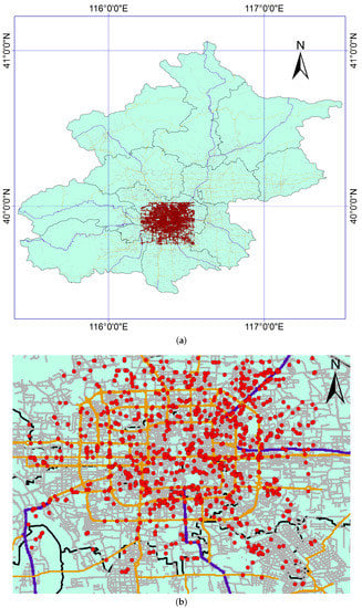
Figure 1.
Selected taxi GPS trajectories in morning rush hours. (a) Overview; (b) An illustration of random 1000 trajectory nodes.
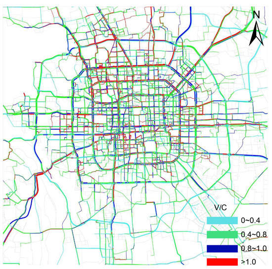
Figure 2.
The V/C of the morning peak during weekdays in Beijing [].
2.3.2. Building of the Primitive Traffic Flow Network
In this step, we aim to build the primitive traffic flow network, which consists of the daily trajectory network of the different taxis and add the weights to the network.
The selected dataset only contains the taxi GPS trajectory nodes, which include the taxi ID, GPS coordinates, and timestamps. To build the trajectory network of each taxi, the following method is employed. First, in terms of the GPS trajectory nodes for each taxi, because taxis are not always in operation, the dataset for the remaining time affects the investigation of the traffic congestion. Thus, we remove the duplicate nodes according to the GPS coordinates and regard each remaining node as a node of the network. Second, we build the edges of the trajectory network for each taxi. Because the trajectory nodes have timestamps, we connect two adjacent nodes chronologically on the same day as the edges. In this manner, we can obtain the primitive traffic flow network. Third, to reflect the real status of the traffic flow, the corresponding weights must be added to the network. In this paper, we aim to investigate traffic congestion; thus, the weights should reflect the congestion status. Based on the GPS coordinates and timestamps of the taxi trajectory data, we introduce the congestion coefficient as the weights of the network []. The congestion coefficient can be defined as:
The distance and duration for an edge can be calculated based on the GPS coordinates and timestamps of the adjacent nodes, respectively. The distance and time are measured in meters and seconds, respectively; thus, the congestion coefficient is measured in s/m. Specifically, the congestion coefficient is the reciprocal of the average velocity through this edge. A larger congestion coefficient corresponds to the smaller speed of a taxi passing through this edge, indicating a higher congestion in the area.
Through this process, the primitive traffic flow network composed of the trajectory network of each taxi can be obtained, which contains the nodes and weighted edges.
2.3.3. Building of the Final Traffic Flow Network
In this step, the primitive traffic flow network is merged with the final traffic flow network. In the primitive traffic flow network, the trajectory networks for the different taxies are independent of one another. Thus, the independent trajectory networks must be merged to build the final traffic flow network. Moreover, as discussed in the previous sections, to investigate traffic congestion problems, the nodes in the traffic flow network should represent the areas. Thus, we can merge the independent trajectory networks through the following method: if several nodes are involved in a common area, the nodes can be replaced by one common node, which can represent an area. Through this process, the independent networks can be merged to create a connected network.
We design a loop algorithm to merge the primitive traffic flow network—(1) for each node of the primitive traffic flow network, a common area is built around the node. In this paper, we design a circular area with a radius of 50 m. If other nodes are involved in the common area, we replace the indexes of these nodes with the index of the node. (2) After the loop, the node list appears as duplicate indexes. Based on the latest node list, for the edge list, we update the nodes’ indexes for the two endpoints of the edge and maintain the weights as constant. Subsequently, the edges with the same endpoints are deleted. (3) We renumber the indexes of the node list and edge list; see Figure 3.
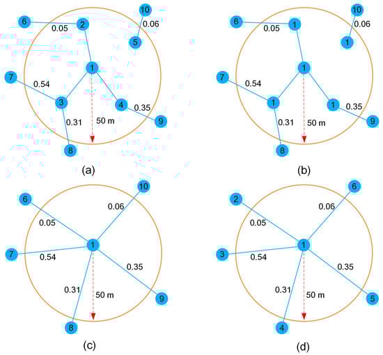
Figure 3.
Merging of the primitive traffic flow network. (a) Original network; (b) Replacement of the indexes (c) Merging of the network; (d) Updating of the indexes.
Finally, we obtain an undirected weighted traffic flow network; see Equation (2)
where represents the nodes set and each node represents a circular area with a radius of 50 m. represents the edges set; is a matrix of weights, where , represents the weights of edges , and the weight can indicate the congestion status.
The traffic flow network we built contains 32,528 nodes and 131,488 edges; see Figure 4.
Figure 4.
A simple illustration of the traffic flow network with 50 edges.
3. Application: Identifying the Congestion Areas for Traffic Planning
3.1. Overview
In this paper, we build a new traffic flow network model to investigate the traffic congestion problems based on taxi GPS trajectories. In the traffic flow network, the nodes represent the real areas, and the edges reflect the congestion status. Moreover, the traffic flow network is scalable and can contain a considerable amount of historical data, thereby ensuring the accuracy of the results.
As mentioned previously, traffic flow networks exhibit the characteristics of complex networks. Thus, certain methods pertaining to the complex network can be applied to the traffic flow network. In a complex network, certain nodes are more important than others [,]. For example, in a healthcare service network, a supply relationship exists between the healthcare service nodes. If an influential node fails, the supply efficiency of the entire healthcare service network is considerably reduced [].
Similarly, in the traffic flow network, the congestion coefficient is employed as the weight of the network. Based on the weights, the nodal attribute values can be obtained by employing different nodal metrics, which can reflect the congestion status of the areas represented by the nodes. Moreover, larger attribute values correspond to a higher congestion of the nodes. Thus, we can identify the congestion areas by ranking the nodal attribute values in descending order.
In this paper, we present a real case based on the traffic flow network. The main task is to identify the congestion nodes by employing different nodal metrics. To identify the congestion nodes in the traffic flow network, the first step is to select proper nodal metrics to calculate the nodal attribute values. Generally, the nodal metrics include local metrics [,,] and global metrics [,,]. For a certain node, the local metrics are used to calculate the nodal attribute values based on the neighboring nodes, while the global metrics are used to calculate the nodal attribute values based on all the other nodes. In real life, traffic congestion often occurs in a local area; thus, the local metrics can more accurately identify the congestion nodes in the traffic flow network.
Serial local weighted metrics, including the nodal strength [], average strength [], weighted clustering coefficient [], and weighted companion behaviors [], are employed to identify the congestion nodes in the traffic flow network. The following text presents the details of the four local nodal metrics.
3.2. Local Weighted Nodal Metrics
3.2.1. Nodal Strength
In an unweighted network, the degree of a node represents the number of neighboring nodes. In a weighted network, the weighted degree of a node is termed as the nodal strength []. The nodal strength is the sum of the weights of the edges connected to the node. The nodal strength can be expressed as in Equation (3).
where represents the nodal strength i, N is the degree of node i, represents the weight of node i and node j.
3.2.2. Average Strength
The average strength [] can be expressed as Equation (4).
where represents the average strength of node i, N is the degree of node i, represents the weight of node i and node j.
The nodal strength and average strength describe the congestion levels in an area from two different perspectives. For a node, the nodal strength and average strength are positively correlated with the congestion levels. Higher nodal and average strength values correspond to a more congested node.
3.2.3. Weighted Clustering Coefficient
To clearly define the weighted clustering coefficient, we first introduce the unweighted clustering coefficient. The unweighted clustering coefficient represents the probability that the neighbors of a node are adjacent to one another, which reflects the compactness of a network []. Suppose node i in a network has edges connecting it to other nodes, and these nodes are neighbors of node i. At most edges can exist between these neighbor nodes. If the actual number of edges between the neighboring nodes is , the unweighted clustering coefficient of node i can be defined as in Equation (5)
where represents the unweighted clustering coefficient of node i. is the actual number of edges between neighbors of node i.
From another perspective, if there exists an edge between the two neighboring nodes of node i, the two neighboring nodes and node i can form a triangle. Thus, is equal to the number of triangles composed of node i and its neighbors, and is equal to the number of connected triples centered on node i; see Figure 5. If the adjacency matrix of the network is , the number of triangles composed of node i and its neighbors is
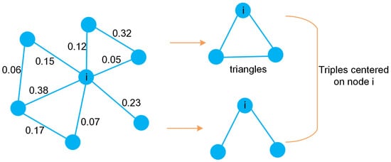
Figure 5.
Illustration of triangles and connected triples.
Thus, can be rewritten as follows; see Equation (7).
In this paper, to reflect the weight of node i, for each triangle composed of node i and its neighbors, we calculate the geometric mean of the normalized weights of the three edges and consider the summation of the weights as the weight of node i []. The weight can be expressed as
where is the weight of node i and node j; , so are and .
Thus, the weighted clustering coefficient can be expressed as
We design an algorithm to obtain . First, we count the number of triangles involved in node i and calculate the geometric mean of the normalized weights of the three edges for each triangle. Second, we sum the aforementioned weights as the weight of node i. Next, we consider the degree of node i as . Finally, we obtain by substituting and in Equation (9).
For example, as shown in Figure 5, there exist three triangles involving node i, and six neighboring nodes, that is, . Thus, of node i can be calculated by summing the weights of the three triangles. Specifically, can be calculated as
Finally, the weighted clustering coefficient .
Note that the numerator and denominator in Equation (9) are zero if the neighbor nodes of node are less than 2. In this case, we set as zero. Moreover, ranges from 0 to 1.
3.2.4. Weighted Companion Behaviors
The companion behaviors [] can reflect the nodal influence through the calculation of the similarity between the node and its neighbors. The Jaccard coefficient () of an edge is employed to reflect the similarity of any connected nodes in the complex network. The of nodes i and j in the unweighted network can be expressed as in Equation (10)
where and represent the neighbors of nodes i and j, respectively; and represent the number of the intersection and unions of the neighbors, respectively. From another perspective, if is not empty, for any node k in , nodes i, j, and k form a triangle. Thus, is also equal to the number of triangles formed by node i and j, and any node in .
The weighted can be calculated as follows. First, we count the number of triangles involving node i and j. Second, for each triangle, we sum the weights of the two edges connected to node i and j. Finally, we sum the weights for all the triangles involving node i and j as the value of weighted . For the weighted , we consider the sum of the nodal strength i and node j. Note that the weight of the edge of node i and j is calculated twice, and the duplicate weight must be removed from the weighted . Subsequently, we can obtain the weighted of node i and j, as .
For example, Figure 6 presents a simple network, for the of node i and node j, the weighted ; the ; thus, the .
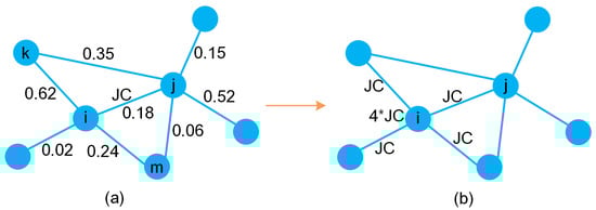
Figure 6.
Illustration of calculation process. (a) of edge ; (b) Companion behaviors of node i.
3.3. Results of Identifying the Congestion Areas
In this section, we aim to identify the congestion nodes in the traffic flow network. To this end, we employ four local nodal metrics, including the nodal strength, average strength, weighted clustering coefficient, and weighted companion behaviors, to identify the congestion nodes. We design an algorithm to conduct this process. First, we calculate the nodal attribute values based on the four different metrics for all the nodes in the traffic flow network. Next, we rank the nodal attribute values in descending order. Larger nodal attribute values correspond to a higher possibility of congestion. The following section presents the results, including those of the statistics of the nodal attribute values, congestion nodes, and evaluation of the four metrics.
3.3.1. Statistics of Nodal Attribute Values
In this paper, we obtain the attribute values of the nodes in the traffic flow network based on the four local weighted metrics. The nodal attribute values can reflect the traffic status of different areas. In this section, we calculate the statistics for the nodal attribute values to investigate the distribution laws of the congestion nodes reflected by the taxi GPS trajectories. Figure 7 presents the frequency distributions of influential values using the local weighted metrics. In Figure 7, the lower curve is the frequency distribution of all data and the upper curve is a local zoom of the first interval. The details are as follows.
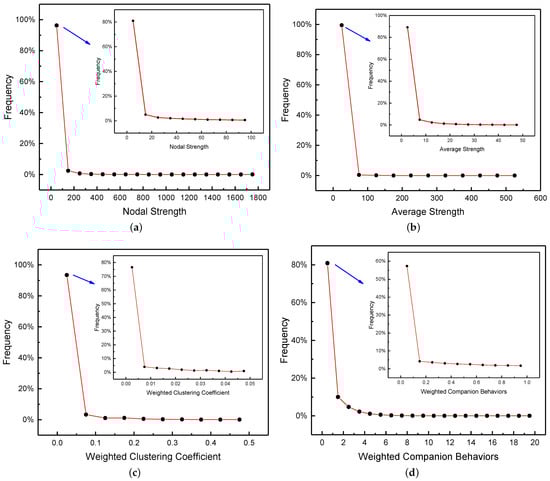
Figure 7.
Frequency distributions of influential values using the local weighted metrics. (a) Nodal Strength; (b) Average Strength; (c) Weighted clustering coefficient; (d) Weighted companion behaviors.
First, the distribution of the nodal strength is 0∼1800, with the maximum and minimum values of 1720.04 and 0.000065, respectively. Moreover, 96.3% and 80.9% of the nodes correspond to values of 0.000065∼100 and 0.000065∼10, respectively, as shown in Figure 7a. Second, the average strength distribution of the nodes is 0∼550, with the maximum and minimum values of 539.56 and 0.000065, respectively. Moreover, 99.5% and 89.2% of the nodes correspond to values of 0.000065∼50 and 0.000065∼5, respectively, as shown in Figure 7b. Third, for the weighted clustering coefficient, the maximum and minimum values are 0.5 and 0, respectively. Moreover, 93.4% and 76.6% of the nodes correspond to values of 0∼0.05 and 0∼0.005, respectively, as shown in Figure 7c. Finally, for the weighted companion behaviors, the maximum and minimum values are 19.1312 and 0, respectively. Moreover, 80.8% and 57.3% of the nodes correspond to values of 0∼1 and 0∼0.1, respectively, as shown in Figure 7d.
The statistical results indicate that for the four local metrics, although the scale of the nodal attribute values of the congestion nodes is different, the distribution of the nodal attribute values exhibits similar trends. Specifically, the distribution of the nodal attribute values is uneven for the four different local metrics. Most nodes are in a lower congestion state, while a few nodes exhibit higher congestion levels, which is consistent with the actual traffic status. Thus, the small number of congestion nodes with higher levels can be identified based on the employed metrics. In the following section, we indicate the congestion nodes with higher levels on the map of Beijing.
3.3.2. Illustration of the Congestion Nodes
To clearly illustrate the results, we select the top 300 congestion nodes based on the nodal attribute values for the different local metrics. Moreover, we mark these nodes on Beijing’s map by using different symbols, with each symbol representing a circular area with a radius of 50 m; see Figure 8.
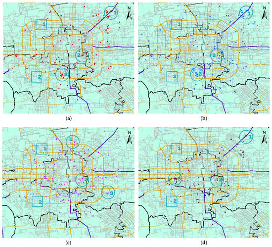
Figure 8.
Distributions of top 300 congestion nodes identified using the weighted metrics. (a) Nodal Strength; (b) Average Strength; (c) Weighted clustering coefficient; (d) Weighted companion behaviors.
The results indicate that the distribution of the top 300 congestion nodes is uneven for the four local metrics. More top congestion nodes exist in certain areas, whereas fewer top congestion nodes exist in the other areas. In real life, certain areas are more congested than the other areas during the morning rush hours in Beijing, such as railway stations and commercial centers. Thus, the distribution of the top 300 congestion nodes is consistent with the traffic status in Beijing.
For each map, we select several areas with more top congestion nodes, and these areas are marked by circles. For example, Figure 8a presents the top 300 congestion nodes identified by the nodal strength. The selected circular areas have more top congestion nodes than those in the other areas. Specifically, circular areas 1∼3 are located around the Beijing airport expressway and Beijing railway station and between the South Third and Fourth Ring Roads. In terms of the average strength, Figure 8b shows that the distribution of the congestion nodes is similar to that of the nodal strength. To verify this aspect, we select three identical circular areas corresponding to the nodal strength. The results indicate that more top congestion nodes exist in these areas, which is consistent with the results of the nodal strength. In the case of the weighted clustering coefficient, circular area 1 is located around the Asian sports village and Anhui overpass, circular area 2 is located around the Beijing railway station, and circular area 3 is located near Beijing Happy Valley; see Figure 8c. In terms of the weighted companion behaviors, the distribution of the congestion nodes is more concentrated than that in the case of the other three metrics. Areas 1 and 2 are located near the Beijing airport expressway and Beijing railway station, respectively, similar to the aforementioned results. In contrast, circular area 3 is located near the Beijing west railway; see Figure 8d.
These results indicate that several congestion areas with high levels can be accurately identified based on the four weighted metrics, including railway stations, airport expressways, and amusement parks. In real life, these locations are key transportation nodes and often experience congestion events, thereby corresponding to more top congestion nodes. The results indicate that the traffic flow network can be used to identify congestion nodes in real life in a reliable manner.
3.3.3. Comparative Evaluation When Using Four Nodal Metrics
In this paper, we consider four local metrics to identify the congestion nodes from different perspectives. The results can reflect the reliability of the four local metrics. For example, all the four local metrics can identify the congestion areas to be within circular area 2. Moreover, three local metrics (nodal strength, average strength, and weighted companion behaviors) identify the congestion areas as being in circular area 1. To verify these findings, we select two areas within the rectangles; see Figure 8. The areas within the rectangles include only a few top congestion nodes. The results of identifying the congestion nodes are thus consistent in the aforementioned areas.
These results demonstrate the similarity of the four metrics in identifying the congestion areas, which reflects the reliability of the four local metrics. Moreover, the results demonstrate the reliability of the traffic flow network.
4. Discussion
In the section, we present the reliablity, advantages, and disadvantages of the traffic flow network. Moreover, the potential further work based on the traffic flow network will be discussed.
4.1. Reliability of the Traffic Flow Network in Identifying the Congestion Areas
In this paper, we build a new traffic flow network model to investigate the traffic congestion problems based on taxi GPS trajectories. Moreover, we apply this network to identify the congestion areas. The results indicate that the traffic flow network is reliable.
First, the datasets are reliable. During the taxi operation, the running route and time are completely determined by the passengers. Thus, taxies can reflect the spatial and temporal rules of the traffic status. Moreover, we extract the taxi GPS trajectory data from 7 a.m. to 9 a.m. from the whole dataset and analyze only the taxi GPS trajectories that appear within the Fifth Ring Road. The selected dataset is sufficiently large and involves sufficient traffic flow, which can contribute to the effective identification of the congestion nodes.
Second, the weights and weighted local nodal metrics of the traffic flow network are reliable. We consider the congestion coefficient as the weight, which can directly reflect the congestion levels based on the reciprocal of the average velocity through the given edge. Moreover, the weighted local nodal metrics are defined based on the weights and can thus reflect the congestion status of the nodes.
Third, based on the traffic flow network, we can identify the key congestion areas in Beijing, such as railway stations, airport expressways, and amusement parks. The results of the real case demonstrate the reliability of the traffic flow network.
4.2. Advantages in the Use of the Traffic Flow Network
In this paper, we build a new traffic flow network model to investigate the traffic congestion problems based on taxi GPS trajectories. In this context, the traffic flow network model involves the following advantages.
First, the traffic flow network based on the taxi GPS trajectories is dynamic and can thus reflect the real traffic status and overcome the limitations pertaining to the use of the static traffic network. Moreover, the traffic flow network is scalable. More datasets can be added to easily build the traffic flow network, which can facilitate the investigation of the traffic congestion. For example, if all the history datasets are employed to identify the congestion areas, we can reliably obtain the congestion areas from a global perspective. In addition, in real life, the congestion nodes may vary due to external factors. We can build different traffic flow networks based on the datasets in different periods. Using these traffic flow networks, we can evaluate the influence of the external factors on the traffic by identifying the changes in the congestion nodes.
Second, for the same dataset, the traffic flow network is changeable and can be used to investigate the congestion problems at different spatial scales. In this paper, we define a circular area with a radius of 50 m as an identification unit, which is sufficiently small in real life. The small identification units can help narrow the identification range of the traffic congestion areas, thereby facilitating the identification of the problems that lead to congestion. By changing the size of the identification units, we can identify the congestion areas from a larger perspective.
Third, as discussed in the previous sections, the traffic flow network has been proven to be reliable.
4.3. Disadvantages in the Use of the Traffic Flow Network
Although the traffic flow network has been proven to be reliable, it involves certain limitations.
First, for the congestion coefficient, the distance of an edge is calculated according to the GPS coordinates, which represent the distance of a straight line. However, due to the change in the taxi driving direction, the real distance between adjacent nodes may be larger than the calculated distance. Moreover, the duration of an edge may contain the waiting time for traffic lights, resulting in a larger traveling time. The congestion coefficient and nodal attribute values may vary in such cases.
Second, although the network based method has been proven to be reliable, the identification results lack the relevant benchmark data. By using the benchmark data, we can adjust the weighted local nodal metrics to match the benchmark data, which can help obtain more accurate metrics. However, it is challenging to obtain the actual benchmark data.
4.4. Outlook and Future Work
In this paper, we build a new traffic flow network model to investigate traffic congestion problems based on taxi GPS trajectories, which can help make decisions in traffic planning. For example, the current dataset can be employed to identify the congestion areas. For these congestion areas, several measures, such as widening urban roads, setting traffic lights, developing public transport systems, and improving the structure of walking networks, can be taken to ease the traffic congestion. Among them, the development of public transport system and the improvement of walking network can reduce the demand for private cars from the source.
Furthermore, the method of building the traffic flow model can be applied to other datasets to investigate novel traffic problems. For example, we can employ the taxi GPS trajectories during evening rush hours to investigate the traffic characteristics. Moreover, we can use the GPS trajectories of private cars or buses to build traffic flow networks that can be used to investigate traffic congestion problems from other perspectives.
Moreover, congestion events are usually related to the static topology of the urban roads. To investigate traffic congestion, the urban static traffic network and dynamic traffic flow network can be combined. In terms of the top congestion nodes, we can determine the relationship between the road topology and traffic congestion to formulate strategies for traffic planning.
In addition, more baseline data must be incorporated in the proposed method, using which, more accurate results can be obtained. Specifically, more new metrics and effective weights can be applied in the traffic flow network to achieve more accurate results. In addition, more analytical methods pertaining to complex networks can be considered to investigate traffic flow networks.
5. Conclusions
In this paper, we build a new traffic flow network model to investigate traffic congestion problems based on taxi GPS trajectories. In the traffic flow network, the nodes represent the real areas, and the weights of the edges reflect the traffic status based on the congestion coefficient. The traffic flow network is scalable and reliable; the approach can be used to analyze traffic congestion problems and provide references for traffic planning. Moreover, to verify the traffic flow network, a real case of identifying the congestion areas is presented. Several local nodal metrics are employed to rank and identify the congestion areas. The results indicate that the traffic flow is reliable. The following research directions can be considered in future work. (1) More new datasets can be employed to build traffic flow networks based on the proposed method, and the new networks can be applied to investigate traffic problems. (2) The urban static traffic network and traffic flow network can be combined to provide suggestions for traffic planning. (3) Additional methods and metrics in the complex network can be applied to the traffic flow network to investigate the traffic problems. The proposed traffic flow network can provide methodological references in traffic planning, especially to solve traffic congestion problems.
Author Contributions
Conceptualization, G.M., J.Q., L.X.; Methodology, J.Q., L.X., G.M.; Writing—Original Draft Preparation, J.Q., G.M.; Writing—Review & Editing, G.M., J.Q. All authors have read and agreed to the published version of the manuscript.
Funding
The research was jointly supported by the National Natural Science Foundation of China (Grant Nos. 11602235), and the Fundamental Research Funds for China Central Universities (2652018091, 2652019220, and 2652019221).
Data Availability Statement
The data presented in this study are available on request from the corresponding author.
Acknowledgments
The authors would like to thank the editor and the reviewers for their helpful comments.
Conflicts of Interest
The authors declare no conflict of interest.
References
- Sussman, J.S. Perspectives on Intelligent Transportation Systems (ITS); Springer: New York, NY, USA, 2005. [Google Scholar] [CrossRef]
- Ahad, A.; Khan, Z.; Ahmad, S. Intelligent Parking System. World J. Eng. Technol. 2016, 4, 160–167. [Google Scholar] [CrossRef]
- Xiang, C.; Liuqing, Y.; Xia, S. D2D for Intelligent Transportation Systems: A Feasibility Study. IEEE Trans. Intell. Transp. Syst. 2015, 16, 1784–1793. [Google Scholar] [CrossRef]
- Xiong, Z.; Sheng, H.; Rong, W.; Cooper, D. Intelligent transportation systems for smart cities: A progress review. Sci. China Inf. Sci. 2012, 55, 2908–2914. [Google Scholar] [CrossRef]
- Zhang, J.; Wang, F.; Wang, K.; Lin, W.H. Data-Driven Intelligent Transportation Systems: A Survey. IEEE Trans. Intell. Transp. Syst. 2011, 12, 1624–1639. [Google Scholar] [CrossRef]
- Porta, S.; Crucitti, P.; Latora, V. The Network Analysis of Urban Streets: A Primal Approach. Environ. Plan. Plan. Des. 2006, 33, 705–725. [Google Scholar] [CrossRef]
- Bin, J.; Christophe, C. Topological analysis of urban street networks. Environ. Plan. B Abstr. 2004, 31, 151–162. [Google Scholar] [CrossRef]
- Porta, S.; Crucitti, P.; Latora, V. The network analysis of urban streets: A dual approach. Phys. A Stat. Mech. Appl. 2006, 369, 853–866. [Google Scholar] [CrossRef]
- De Montis, A.; Barthelemy, M.; Chessa, A.; Vespignani, A. The structure of Inter-Urban traffic: A weighted network analysis. Environ. Plan. B Plan. Des. 2007, 34, 905–924. [Google Scholar] [CrossRef]
- Stefan, L.; Bjorn, G.; Helbing, D. Scaling laws in the spatial structure of urban road networks. Phys. A Stat. Mech. Appl. 2006, 363, 89–95. [Google Scholar] [CrossRef]
- Paolo, C.; Vito, L.; Sergio, P. Centrality measures in spatial networks of urban streets. Phys. Rev. E 2006, 73. [Google Scholar] [CrossRef]
- Leung, X.; Chan, S.Y.; Hui, P.; Lio, P. Intra-City Urban Network and Traffic Flow Analysis from GPS Mobility Trace. Phys. Soc. 2011, 12, 1047–1056. [Google Scholar] [CrossRef]
- Zhong, G.; Yin, T.; Zhang, J.; He, S.; Ran, B. Characteristics analysis for travel behavior of transportation hub passengers using mobile phone data. Transportation 2018, 46, 1713–1736. [Google Scholar] [CrossRef]
- Zhang, S.; Tang, J.; Wang, H.; Wang, Y.; An, S. Revealing intra-urban travel patterns and service ranges from taxi trajectories. J. Transp. Geogr. 2017, 61, 72–86. [Google Scholar] [CrossRef]
- Tao, D.; Zhi-Ming, C.; Zhe, C.; Jun, K. Analysis of Taxi Passenger Travel Characteristics Based on Spark Platform. Comput. Syst. Appl. 2017, 3, 37–43. [Google Scholar] [CrossRef]
- An, S.; Yang, H.; Wang, J. Revealing Recurrent Urban Congestion Evolution Patterns with Taxi Trajectories. ISPRS Int. J. Geo-Inf. 2018, 7, 128. [Google Scholar] [CrossRef]
- Kan, Z.; Luliang, T.; Kwan Mei-Po, R.; Chang, L.; Dong, L.; Qingquan, L. Traffic congestion analysis at the turn level using Taxis’ GPS trajectory. Comput. Environ. Urban Syst. 2019, 74, 229–243. [Google Scholar] [CrossRef]
- Liu, C.; Wang, S.; Cuomo, S.; Mei, G. Data analysis and mining of traffic features based on taxi GPS trajectories: A case study in Beijing. Concurr. Comput. Pract. Exp. 2019. [Google Scholar] [CrossRef]
- Wenhuan, S. A Taxi-Tracking-based Method for Traffic Status Estimation of Urban Road-Network. J. Transp. Inf. Saf. 2009, 5, 29–32. [Google Scholar]
- Li, S.; Wu, J.; Gao, Z.Y.; Lin, Y.; Fu, B. The analysis of traffic congestion and dynamic propagation properties based on complex network. Acta Phys. Sin. 2011, 60. [Google Scholar] [CrossRef]
- Wu, J.; Sun, H.; Gao, Z. Dynamic urban traffic flow behavior on scale-free networks. Phys. A Stat. Mech. Appl. 2008, 387, 653–660. [Google Scholar] [CrossRef]
- Wang, S.; Cuomo, S.; Mei, G.; Cheng, W.; Xu, N. Efficient method for identifying influential vertices in dynamic networks using the strategy of local detection and updating. Future Gener. Comput. Syst. 2019, 91, 10–24. [Google Scholar] [CrossRef]
- Salavati, C.; Abdollahpouri, A.; Manbari, Z. Ranking nodes in complex networks based on local structure and improving closeness centrality. Neurocomputing 2018. [Google Scholar] [CrossRef]
- Fornito, A.; Zalesky, A.; Bullmore, E.T. Fundamentals of Brain Network Analysis; Academic Press: Cambridge, MA, USA, 2016. [Google Scholar] [CrossRef]
- Tripathy, R.M.; Bagchi, A.; Jain, M. Complex Network Characteristics and Team Performance in the Game of Cricket. In Big Data Analytics; Springer International Publishing: Berlin/Heidelberg, Germany, 2013; pp. 133–150. [Google Scholar]
- Saramaki, J.; Kivela, M.; Onnela, J.P.; Kaski, K.; Kertesz, J. Generalizations of the Clustering Coefficient to Weighted Complex Networks. Phys. Rev. E 2007, 75, 027105. [Google Scholar] [CrossRef] [PubMed]
- Zheng, Y.; Tang, L.A.; Han, J.; Leung, A.; Hung, C.C.; Peng, W.C.; Yuan, J.; Yuan, N.J. On Discovery of Traveling Companions from Streaming Trajectories. In Proceedings of the 28th International Conference on Data Engineering, Arlington, VA, USA, 1–5 April 2012. [Google Scholar]
- Yuan, N.J.; Zheng, Y.; Xie, X.; Sun, G. T-Drive: Enhancing Driving Directions with Taxi Drivers’ Intelligence. IEEE Trans. Knowl. Data Eng. 2013, 25, 220–232. [Google Scholar] [CrossRef]
- Center, B.T.D.R. Annual Report of Beijing Traffic Development in 2009. 2009. Available online: http://www.bjtrc.org.cn/List/index/cid/7/p/2.html (accessed on 25 October 2020).
- Liu, D.; Jing, Y.; Chang, B. Identifying influential nodes in complex networks based on expansion factor. Int. J. Mod. Phys. C 2016, 27, 1650105. [Google Scholar] [CrossRef]
- Bian, T.; Hu, J.; Deng, Y. Identifying influential nodes in complex networks based on AHP. Phys. A Stat. Mech. Appl. 2017, 479, 422–436. [Google Scholar] [CrossRef]
- Qi, X.; Mei, G.; Cuomo, S.; Xiao, L. A network-based method with privacy-preserving for identifying influential providers in large healthcare service systems. Future Gener. Comput. Syst. 2020, 109, 293–305. [Google Scholar] [CrossRef]
- Lu, L.; Zhou, T.; Zhang, Q.M.; Stanley, H.E. The H-index of a network node and its relation to degree and coreness. Nat. Commun. 2016, 7, 10168. [Google Scholar] [CrossRef]
- Jing, F.; Zhuo-qiong, Q.; Guo-qing, Z. A Method for Improving Complex Network Capacity Based on Betweenness Centrality. Comput. Simul. 2008, 25, 167–170. [Google Scholar]
- Fei, L.; Zhang, Q.; Deng, Y. Identifying influential nodes in complex networks based on the inverse-square law. Phys. A Stat. Mech. Appl. 2018, 512, 1044–1059. [Google Scholar] [CrossRef]
- Arruda, D.; Ferraz, G. Role of centrality for the identification of influential spreaders in complex networks. Phys. Rev. E 2014, 90. [Google Scholar] [CrossRef] [PubMed]
- Wu, X.; Li, X.; Chen, R. Network Science: An Introduction; Higher Education Press: Beijing, China, 2012. [Google Scholar]
Publisher’s Note: MDPI stays neutral with regard to jurisdictional claims in published maps and institutional affiliations. |
© 2020 by the authors. Licensee MDPI, Basel, Switzerland. This article is an open access article distributed under the terms and conditions of the Creative Commons Attribution (CC BY) license (http://creativecommons.org/licenses/by/4.0/).