Thermo-Environmental Assessment of a Heated Venlo-Type Greenhouse in the Yangtze River Delta Region

Abstract

Accurate evaluation of microclimate conditions in a greenhouse can assist producers to manage crop production and designers to optimize climate control systems. An assessment of the variable thermo-environmental behavior of a heated Venlo-type greenhouse under the influence of naturally changing climate conditions in the Yangtze River Delta region was undertaken. A three-dimensional transient computational fluid dynamics (CFD) model was developed to analyze the airflow pattern and dynamic distribution of temperature and humidity inside the greenhouse. Validation of the numerical model showed a satisfactory agreement between measured and simulated values of air velocity, temperature, and absolute humidity, with mean hourly air temperature mean absolute error (MAE) and root mean square error (RMSE) values of $7.7\%$ and $7.9\%,$ respectively, and mean hourly air humidity MAE and RMSE values of $16.18\%$ and $16.42\%,$ respectively. Simulation results demonstrated that the airflow pattern shaped the distribution of temperature and absolute humidity, and homogeneity of both variables was prevalent inside the greenhouse. These results could be adopted by growers and designers in the Yangtze River Delta region and other sub-tropical climatic regions to improve crop production and optimize climate control systems.

1. Introduction

In the Yangtze River Delta region of China, greenhouses are rarely equipped with environmental control systems due to the high installation, operational, and maintenance costs of these systems, which are exacerbated by an ever-increasing energy cost [1]. Consequently, the closed greenhouse approach is generally applied during winter in this sub-tropical monsoon climate. Closed greenhouses depend on passive absorption of solar energy through seasonal storage to maintain a suitable crop growth environment. Nevertheless, this method is not feasible particularly when temperatures sink below the biological optimum for plant growth. To prevent crop-damage economic losses caused by cold stress, growers are usually obliged to employ fossil fuel-based energy sources to power heaters to maintain suitable inside temperatures. Combustion of these non-renewable energy sources produces large quantities of CO, CO₂, SO₂, and NO_x, which are chronic air pollutants leading to environmental degradation [2].

In the semi-closed greenhouse approach, semi-closed greenhouses with active climate control systems are designed for sustainable energy solutions. Although the initial installation outlay might be high, the expected benefits in terms of low energy cost, zero economic loss from crop damage, and higher production yield makes the investment cost-effective in the long term. Furthermore, with the recent advancements in renewable energy sources and an upsurge in government incentives, there has been an increased willingness by potential growers in this region to integrate renewable energy with climate control systems, as was the case with the greenhouse under study. Use of renewable energy sources reduces carbon emissions, which has a positive impact on the environment [3]. This is especially significant in this region with a severe air pollution problem and rapid urbanization, which has led to a sharp decline in croplands [4], leading to greenhouse facilities gradually becoming the primary form of agricultural activity. Scholars have utilized renewable energy sources for greenhouse heating as a replacement for fossil fuel-based energy sources. Benli et al. [5] used a ground-source heat pump system with latent heat storage, Kumar et al. [6] utilized biogas, and Esen et al. [7] employed a biogas, solar, and ground-source heat pump system.

In semi-closed greenhouses, the two microclimate parameters that are crucial to an optimum greenhouse microclimate are temperature and humidity. These variables are extremely sensitive to the dynamic behavior of outside climate conditions. Outside climatic conditions, which include air temperature, solar radiation, and the wind regime, affect the radiation, convection, and conduction heat transfer between the exterior and interior of the greenhouse. Therefore, accurate assessment of these variables is essential, especially under the influence of external climatic conditions.

Computational fluid dynamics (CFD) is a numerical tool that has been applied by researchers to study the microclimate conditions in greenhouses. CFD has been used to investigate optimum greenhouse design and ventilation optimization [8], greenhouse air leakage [9], model micrometeorology, and irrigation strategies [10,11].

Heated semi-closed greenhouses have been extensively studied [12,13]; however, few studies have applied CFD to investigate the spatial and transient variation of microclimate parameters inside these greenhouses. Tadj et al. [14] utilized CFD to study steady-state spatial distribution of climate variables inside a heated round arch greenhouse in eastern Greece and the 2-D CFD model revealed that the air heater resulted in the greenhouse air volume being split into two regions: crop level and above-crop level. Natural convection was prevalent in the crop-level region and forced or mixed convection mode was dominant at the above crop-level region depending on relative distance from the air heater. The authors recorded a mean error of 16% between measured and simulated values for air velocity, air temperature, and absolute air humidity. The 3-D CFD model developed by Boulard et al. [10] to predict steady-state spatial distribution of temperature, water vapor, and CO₂ in a heated Venlo-type greenhouse in the south of France registered fair agreement with the measured variables and showed homogeneous vertical and horizontal patterns of air temperature, humidity, and CO₂ in the greenhouse. Under Mediterranean climatic conditions, Cuoto et al. [15] carried out a 2-D CFD simulation of a heated arc-type greenhouse to investigate the steady-state spatial distribution of indoor temperature and air velocity. Very good agreement was obtained between the experimental and simulated values. Flores-Velázquez et al. [16] employed a 3-D CFD model to investigate steady-state spatial air dynamics and temperature behavior in a single bay of a pipe-heated Venlo-type greenhouse in Germany. The CFD model depicted a convective airflow from the center of the greenhouse bay to the walls with a marked temperature gradient close to the soil. A non-uniform temperature pattern was observed even in low wind speeds. Airflow and temperature distribution in a tunnel greenhouse with heating pipes was analyzed by Zeroual et al. [17] using CFD to investigate pure convective and radiative–convective thermal losses at the greenhouse cover. The streamlines and isotherms generated by the 2-D steady-state CFD model displayed the variation of temperature gradient inside the greenhouse under the different boundary conditions evaluated.

Transient CFD numerical studies undertaken by scholars have mainly focused on naturally ventilated greenhouses. Nebbali et al. [18] investigated the 3-D distribution of climate variables within a naturally ventilated tunnel greenhouse considering dynamic exterior environmental conditions. The investigations found that the wind regime strongly influenced the difference between the inside and outside temperatures, as it reached $12 ℃$ for low wind conditions but only $6 ℃$ on the same day for high wind conditions. In contrast, a moderate influence of wind velocity on the inside relative humidity of less than $10\%$ was observed. Villagrán et al. [19] investigated 2-D transient variation of temperature and air velocity in three naturally ventilated greenhouses in the high Andean tropics and observed a homogeneous thermal spatial distribution in the curved multi-span design and gothic multi-span design greenhouses as compared to the traditional Colombian greenhouse due to higher ventilation rates. Tong et al. [20] employed CFD to predict temperature distributions inside a Chinese solar greenhouse considering transient boundary conditions. The authors observed that the mean temperature differences between the nighttime measured and simulated air temperatures was less than $1 ℃$ on clear days, and not more than $1.5 ℃$ on a cloudy day. Fidaros et al. [21] simulated the 2-D transient transport phenomena in an arc-type greenhouse under the influence of constant and dynamic outside temperature, and the results underscored the significance of considering external temperature variation.

According to the authors’ best knowledge, currently there are no CFD studies that analyze the spatial and transient variation of microclimate parameters inside a heated semi-closed greenhouse. Furthermore, there is little information in the literature at present on three-dimensional climate distribution inside semi-closed greenhouses. For this reason, there is an imperative need for a study that analyzes the 3-D spatial and transient variation of greenhouse microclimate variables and factors in the influence of dynamic outside climate conditions.

Therefore, in this research, a 3-D transient CFD model was developed to investigate the spatial and transient variation of microclimate parameters inside a heated greenhouse, under the influence of naturally changing climate conditions that exist outside the greenhouse in the Yangtze River Delta region during the winter period. The results obtained in this study could be adopted by producers and designers in this region and other sub-tropical climatic regions in the world to improve crop production and optimize climate control systems.

This leads to the research hypotheses in this study: to refute or confirm that (1) the developed CFD model has the capability to predict the air velocity, temperature, and humidity behavior in a heated Venlo-type greenhouse; that (2) the 3-D transient model allows for a detailed assessment of the spatio-temporal distribution of the microclimate variables; that (3) the airflow pattern inside the greenhouse has an influence on the spatial distribution of temperature and humidity; and that (4) utilization of multiple air heaters would result in a homogeneous microclimate within the greenhouse.

2. Methodology

2.1. Modeling and Numerical Simulation

2.1.1. Governing Equations

Transient distribution of mass, velocity components, temperature, and water vapor within the computational domain, represented by the distribution of the physical parameter $\varnothing ,$ is governed by the classical transport equation. The general form of the transport equation may be written as:

$$\frac{\partial \varnothing }{\partial t}+\frac{\partial }{\partial x_j}\left(u_j\varnothing \right)=\frac{\partial }{\partial x_j}\left({\Gamma }_{\varnothing }\frac{\partial \varnothing }{\partial x_j}\right)+S_{\varnothing }$$

(1)

where $\varnothing$ is the concentration of the variable transported in dimensionless form, t is time, u_j is the velocity component, x_j is the coordinate in the x, y, and z directions of the Cartesian space, ${\Gamma }_{\varnothing }$ is the diffusion coefficient of the variable ∅, and $S_{\varnothing }$ is the source term of the variable ∅.

2.1.2. Turbulence Model

The Rayleigh number R_a is a dimensionless number that is related to airflow driven by buoyancy and is calculated using the equation:

$$R_a=Pr\ast Gr=\frac{g\rho \beta \Delta T_{c,r}{H}^3}{\alpha \mu }$$

(2)

where $Pr \mathrm{and} Gr$ are the Prandtl number and Grashof number, respectively, $g$ is the acceleration due to gravity, $\rho$ is density of the fluid, $\beta$ is the thermal expansion coefficient, $\mathsf{\Delta }{T}_{c,r}$ is the maximum temperature difference of the airflow between the canopy and greenhouse roof surface, $H$ is the characteristic height of the greenhouse, $\alpha$ is the thermal diffusivity, and $\mu$ is the kinematic viscosity. Forced-air ventilation is usually expected to increase the Rayleigh number values to R_a > 10¹⁰ in a large enclosed greenhouse envelope, with flow exceeding the threshold value at which the transition to turbulence occurs over the range of $R_a\cong {10}^8~{10}^{10}$. However, not all points within the greenhouse exist in the region of full turbulence. In a bid to accommodate this phenomenon and accurately reproduce the realistic convective flows, the model incorporated the Lam–Bremhorst low-Reynolds number k-ε turbulence model [22], given by:

$$u\frac{\partial \left(\rho k\right)}{\partial x}+v\frac{\partial \left(\rho k\right)}{\partial y}+w\frac{\partial \left(\rho k\right)}{\partial z}=\mu +\frac{\mu }{{\sigma }_k}+\left(\frac{{\partial }^{2}k}{\partial x^2}+\frac{{\partial }^{2}k}{\partial y^2}+\frac{{\partial }^{2}k}{\partial z^2}\right)+{\mu }_t\rho \left(P-G_B\right)-\rho \epsilon$$

(3)

$$u\frac{\partial \left(\rho \epsilon \right)}{\partial x}+v\frac{\partial \left(\rho \epsilon \right)}{\partial y}+w\frac{\partial \left(\rho \epsilon \right)}{\partial z}=\mu +\frac{\mu }{{\sigma }_{\epsilon }}+\left(\frac{{\partial }^2\epsilon }{\partial x^2}+\frac{{\partial }^2\epsilon }{\partial y^2}+\frac{{\partial }^2\epsilon }{\partial z^2}\right)+C_1{\mu }_t\rho \frac{\epsilon }{k}\left(f_{1}P-G_B\right)-C_2{f}_2\rho \frac{{\epsilon }^2}{k}$$

(4)

where u, v, and w are the velocity components in the x, y, and z directions, $k$ is the kinetic energy of turbulence, $\epsilon$ is the dissipation of turbulent kinetic energy, ${\mu }_t$ is the turbulent viscosity ${\sigma }_k$, ${\sigma }_{\epsilon }$ is the Prandtl number of the turbulent kinetic energy k and dissipation rate $\epsilon ,$ respectively, $G_B$ is the generation of turbulent kinetic energy due to buoyancy, and P is the calculated pressure.

Auxiliary relations required for a successful solution are:

Turbulent eddy viscosity ${\mu }_{t,}$ computed by combining $k$ and $\epsilon$ [23]:

$${\mu }_t=c_{\mu }\rho f_{\mu }\frac{k^2}{\epsilon }$$

(5)

where $f_{\mu }$ is the damping function that depresses the effect of near-wall turbulence;

Turbulent kinetic energy production $G_{B,}$ given by [24]:

$$G_B=\frac{g\beta }{\rho {\sigma }_t}\frac{\partial \left(T-T_{ref}\right)}{\partial y}$$

(6)

where $\beta$ is the thermal coefficient of volumetric expansion, defined as:

$$\beta =\frac{1.0}{T_{ref}}$$

(7)

and $T_{ref}$ is the reference temperature and ${\sigma }_t$ the turbulent Prandtl number;

Calculated pressure P, given by:

$$P=\left(\frac{u_i}{\partial x_j}+\frac{u_j}{\partial x_i}\right)\frac{u_i}{\partial x_j}$$

(8)

Damping functions $f_1$, $f_2,$ and $f_{\mu },$ defined as [23,25]:

$$f_1=1.0+{\left(\frac{0.05}{f_{\mu }}\right)}^3$$

(9)

$$f_2=1.0-e^{-R{e}_t^2}$$

(10)

$$f_{\mu }={\left(1.0-e^{-0.0165R{e}_k}\right)}^2\left(1.0+\frac{20.5}{R{e}_t}\right)$$

(11)

$$R{e}_k=\frac{k^{1/2}\rho y}{\mu }$$

(12)

$$R{e}_t=\frac{k^2\rho }{\mu \epsilon }$$

(13)

where $R{e}_t$ is the Reynolds number related to turbulent conditions, $R{e}_k$ is the Reynolds number related to turbulent conditions as a function of the location relative to the nearest solid boundary, and y is the generalized normal distance from a solid boundary. The turbulence model constants were ${\sigma }_t$ = 0.90, ${\sigma }_k$ = 1.00, ${\sigma }_{\epsilon }$ = 1.30, $C_{\mu }$ = 0.09, C₁ = 1.44, and C₂ = 1.92 [22,23].

Equations ($5$)–($13$) are substituted into Equations ($3$) and ($4$) to incorporate the Lam–Bremhorst low-Reynolds number k–ε turbulence model.

2.1.3. Radiation Model

The radiation sub-model was activated to map the thermal contribution of radiative transfers [26]. The discrete ordinates model (DOM) was adopted to model radiation [27]. The DOM solves the radiative transfer equation (RTE) for a finite number of discrete solid angles, each associated with a vector direction $\overrightarrow{s}$ fixed in the global Cartesian system x, y, and z. The RTE is transformed by the DOM into a radiation intensity transport equation in the x, y, and z spatial coordinates. The RTE for spectral radiative intensity in the DOM in the optical direction $\overrightarrow{s}$ is considered as a field equation and for a given wavelength is defined as [28]:

$$\nabla ·\left(I_{\lambda }\left(\overrightarrow{r},\overrightarrow{s}\right)\overrightarrow{s}\right)+\left(a_{\lambda }+{\sigma }_s\right)I_{\lambda }\left(\overrightarrow{r},\overrightarrow{s}\right)=a_{\lambda }{n}_{\lambda }^2\frac{{\sigma T}^4}{\mathsf{\pi }}+\frac{{\sigma }_s}{4\mathsf{\pi }}\underset{0}{\overset{4\mathsf{\pi }}{\int }}{I}_{\lambda }(\overrightarrow{r},{\overrightarrow{s}}^{\prime })\mathsf{\Phi }(\overrightarrow{s}·{ \overrightarrow{s}}^{\prime }){d\Omega }^{\prime }$$

(14)

where $\nabla$ is the divergent operator, $\lambda$ the radiation wavelength, $a_{\lambda }$ the spectral absorption coefficient of the participating medium, ${\sigma }_s$ the spectral scattering coefficient of the participating medium, $\overrightarrow{r}$ the position vector, $\overrightarrow{s}$ the directional vector, $I_{\lambda }$ the spectral intensity of the radiation (which is dependent on the position $\overrightarrow{r}$ and direction $\overrightarrow{s}$), n the index of refraction, T the local temperature, ${\overrightarrow{s}}^{\prime }$ the scattered vector with the direction of the ray originating from the direction $\overrightarrow{s}$, $\mathsf{\Phi }$ the scattering phase function, and $d{\Omega }^{\prime }$ the solid angle of radiation.

2.1.4. Crop-Zone Sub-Model

The crop zone within the greenhouse was modelled as a homogeneous porous medium to simplify the complexities associated with the crop canopy. The crop zone applied a mechanical resistance to the fluid flow and coupled with the mass and heat balance of the air in the greenhouse [29]. The pressure drop induced by the crop-zone resistance to fluid flow movement is accommodated in the Navier–Stokes equations using the Darcy–Forchheimer equation. The source term $S_{\varnothing }$ in the momentum equation comprises viscous loss term and inertial resistance.

The source term is defined as:

$$S_{\varnothing }=-\left({\mu C}_1+\frac{1}{2}{C}_2{\rho }_{a}u\right)u$$

(15)

where $\mu$ is the kinematic viscosity of air, $C_1$ is the inverse of permeability of the porous medium, $u$ is the velocity magnitude of air, $C_2$ is the non-linear momentum loss coefficient, and ${\rho }_a$ is the air density.

Pressure loss due to the viscous resistance is negligible compared to the pressure decrease due to the inertial resistance because the kinematic viscosity of air is very low, in the order of ${10}^{-5}$. As such, the viscous loss term can be neglected [30] and the momentum sink consequently depends on the inertial resistance. The sink of momentum in the transport equation, Equation ($1$), is due to the drag effect of the crop canopy. The Wilson equation [31], which defines the relationship between the crop drag coefficient and the associated pressure reduction, is applied to estimate the inertial resistance of the crop canopy as:

$$S_{\varphi }=-{\rho }_a{LAD}_v{C}_D{u}^2$$

(16)

where $LA{D}_v$ is the volumetric leaf area density and $C_D$ is the drag coefficient.

Equating Equations ($15$) and ($16$), the relationship between $C_D$ and $C_2$ is deduced as:

$$C_2=2{LAD}_v{C}_D$$

(17)

A $C_D$ value of 0.32 [32] was adopted for this study.

The thermal balance on the leaf describes the exchange of heat and water vapor between the leaves and greenhouse air and is written as:

$$R_{net}-Q_{lat}-Q_{sen}=0$$

(18)

where $R_{net}$ is the net radiation on the leaf, $Q_{lat}$ is the latent heat exchange due to leaf transpiration, and $Q_{sen}$ is the sensible heat exchange.

Net solar radiation received at each control volume of the canopy at an arbitrary height y is deduced by Beer’s law:

$$R_{net}={Rg}_o\exp \left(-k_c\ast LAI\ast \frac{h-y}{h}\right)$$

(19)

where $R{g}_o$ is the global solar radiation above the canopy, $k_c$ is the extinction coefficient of radiation estimated at a value of 0.95 [32], $h$ is the total height of the canopy, and $LAI$ is the leaf area index.

The sensible heat flux at the leaf level was given by the equation:

$$Q_{sen}=2{\rho }_a{C}_p\frac{T_{leaf}-T_a}{r_a}$$

(20)

where ${\rho }_a$ is the density of air, $C_p$ is the specific heat of air under constant pressure, $T_{leaf}$ and $T_a$ are the temperatures of leaf and air, respectively, and $r_a$ is the aerodynamic resistance.

The transpiration rate for a given control volume was given by [33]:

$$Q_{lat}=\frac{{\mathrm{R}}_{net}·\Delta +\left(\left(2{LAI\rho }_a{C}_p\right)/r_a\right)VPD}{\gamma ·(1+\left(\Delta /\gamma \right)+\left(r_s/r_a\right)}$$

(21)

where $VPD$ is the vapor pressure deficit of air, $\Delta$ is the slope of the saturated water vapor pressure curve according to temperature, $\gamma$ is the psychrometric constant, and $r_s$ is the stomatal resistance.

The aerodynamic resistance $r_a$ was calculated using the relationship [10]:

$$r_a=305\frac{l}{\sqrt{u+{\left(g\beta \left|T_{leaf}-T_a\right|l\cos \theta \right)}^{0.5}}}$$

(22)

where l is the characteristic length of the leaf and $\theta$ is the average angle between the leaf and the horizontal plane, assumed to be at $0°$ when leaf surfaces are saturated. The stomatal resistance $r_s$ was calculated for each control volume in the canopy domain using the equation [34]:

$$r_s=C_3·\left(\frac{(R_{net}/\left(2LAI\right))+C_4}{(R_{net}/\left(2LAI\right))+C_5}\right)·\left(1+C_6·{VPD}^2\right)$$

(23)

where $C_3, C_4, C_5, \mathrm{and} C_6$ are constants equal to 80.8, 14.3, 0.44, and $1.9\times {10}^{-6}$, respectively.

Leaf temperature can be deduced from Equation ($18$) to give:

$$T_{leaf}= \frac{r_a}{2{\rho }_a{C}_p}·\left(R_{net}-Q_{lat}\right)+T_a$$

(24)

2.2. Numerical Model and Mesh Generation

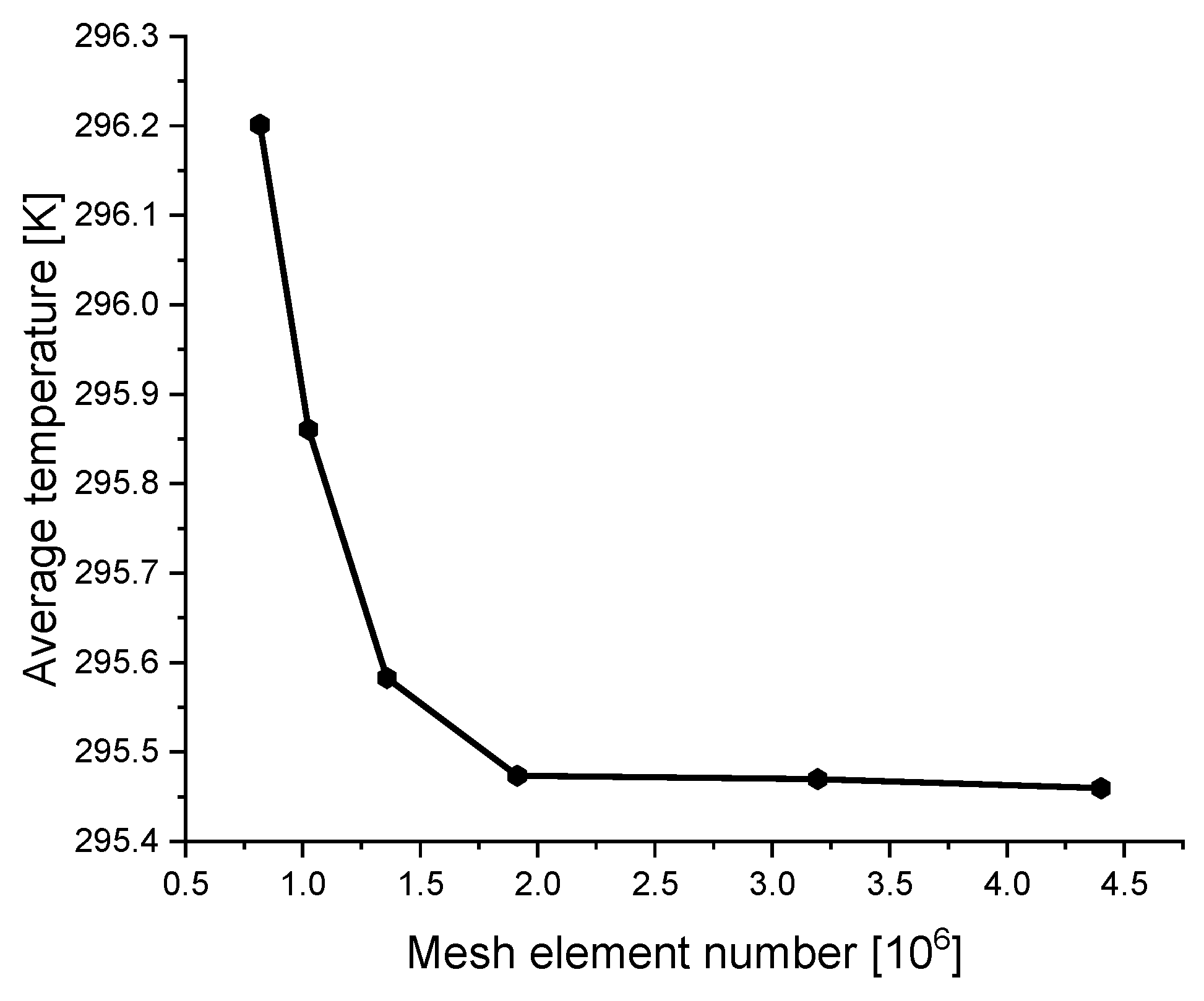
2.2.1. Mesh Generation

ANSYS 2020 R1 (ANSYS Inc., Canonsburg, PA, USA) component packages: SpaceClaim was used to design the greenhouse geometry and Integrated Computer Engineering and Manufacturing (ICEM) CFD for mesh generation. ICEM tools parametrically divided the computational domain into unstructured tetrahedral/mixed meshes with a total of 4,400,904; 3,193,527; 1,914,098; 1,358,372; 1,024,834; and 817,789 elements, a consequence of progressively increasing the maximum element face size by 0.05 m from 0.25 m to 0.5 m, a best practice recommended by Ansys [28]. An increment in the number of elements within the computational domain will always obtain accurate and reliable results, to an extent. Thereafter, a more refined mesh may not necessarily improve the accuracy of the simulation results. Therefore, there is need to carry out a mesh independence test to verify that the numerical results are independent of the mesh size. Steady-state simulations were carried out using the boundary conditions between 9:00 and 10:00 h to analyze the effect of increasing the number of mesh elements on the variation of average greenhouse air temperature. The optimal mesh size is identified when there is a negligible deviation in the air temperature with an increase in mesh elements. The results for the mesh independence test are as shown in Figure 1.

Figure 1 depicts a significant decrease in the average air temperature as the mesh elements increased from 817,789 to 1,914,098. There was negligible variation in the air temperature as the mesh elements increased from 1,914,098 to 4,400,904. The 3,193,527-element mesh was adopted for this study, as a finer mesh would provide sufficient accuracy for capturing 3-D spatial distribution of the variables within the entire computational domain [28].

2.2.2. Numerical Model

Ansys Fluent^TM 2020R1 was used to carry out three-dimensional transient simulations using the finite volume method. This numerical simulation tool solves the unsteady 3-D Navier–Stokes conservation equations for energy, mass, and momentum. Radiation transfers and crop-zone models were also integrated into the model.

• Boundary and Initial Conditions

The time evolution of greenhouse exterior climate parameters constituted the dynamic climatic conditions that were applied as boundary conditions to the greenhouse domain. The boundary conditions were inferred from sensor measurements of greenhouse exterior air temperature, solar radiation, and wind speed. Temperature $T_o$, solar radiation intensity $R{g}_o$, and wind speed $U_o$ were as provided in Figure 2.

Initial conditions were also extracted from sensor measurements of air temperature and humidity inside the greenhouse and field measurements of air temperature, solar radiation, and wind speed outside the greenhouse.

The greenhouse was equipped with 83 fan coil units (FCUs). The discharge vents of the fans were modeled as velocity inlet. A fixed velocity of 5 ms⁻¹ and an isothermal condition of 303.15 K was imposed at the inlets. The horticultural glass cover of the greenhouse, which makes up the stationary walls and the roof, takes part in both convection and radiation. It was treated as a semi-transparent medium and assigned a non-slip, mixed thermal boundary condition. Its heat transfer coefficient was calculated using the equation [35]:

$$H_c=5.2+3.8\times U_o$$

(25)

where $H_c$ is the heat transfer coefficient and $U_o$ is the external wind speed.

The concrete floor was modelled as a diffusively radiating opaque boundary, as was recommended by Dhiman et al. [36]. The external radiation temperature was deduced as the average of the sky temperature $T_{sky}$ and greenhouse outside temperature $T_o$. The sky temperature $T_{sky}$ was computed according to the equation [37]:

$$T_{sky}=0.0552T_o^{1.5}$$

(26)

2.

Numerical method

The semi-implicit method for pressure linked equations (SIMPLE) was used to solve the coupled pressure–momentum equations. The second-order upwind discretization scheme was used for momentum, turbulence, water vapor, energy, and discrete ordinates (DO) transport equations because the higher-order schemes result in greater accuracy.

The model convergence criteria for the residuals were reduced to 10⁻⁶ for better accuracy of the simulation results. The settings adopted for the CFD simulations, including the relaxation factors, are shown in

Table 1. Parameters for the computational fluid dynamics (CFD) simulations.

CFD Component	Method/Parameter/Setting
Solver settings	3-D transient simulation
Scheme	SIMPLE* scheme, pressure-velocity coupling
Gradient discrete scheme	Green–Gauss node based 1
Pressure discrete scheme	Body force weighted method 2
Momentum, k and $\epsilon$, water vapor, energy, and discrete ordinates scheme	Second-order upwind scheme
Transient formulation	Bounded second-order implicit 3
Relaxation factors
Pressure	0.3
Density	1
Body force	0.9
Momentum	0.7
k and $\epsilon$	0.7
Turbulent viscosity	0.8
Water vapor	0.7
Energy	0.8
DO	0.8
Models
Radiation	Discrete ordinates model Theta and phi divisions: 3 Theta and phi pixels: 3 Energy iterations per radiation iteration: 10
Species	Mixture of dry air and water vapor

¹ Green–Gauss node based: node-based gradient discrete scheme that applies the Green–Gauss method; ² body force weighted method: the recommended pressure discrete scheme for problems involving large body forces; ³ bounded second-order implicit: ensures second-order accuracy that is bounded to limit production of non-physical oscillations. *SIMPLE: semi-implicit method for pressure linked equations.

. Physical and optical properties of materials within the computational domain adopted for the simulations are summarized in

Table 2. Physical and optical material properties.

Property	Glass	Water Vapor	Air	Concrete Floor
Density	2500	0.5542	1.225	2300
Specific heat	840	f(T)*	1006.43	2300
Thermal conductivity	1.2	0.0261	0.0242	1.4
Absorption coefficient	-	0.54	0.19	0.92
Scattering coefficient	-	-	-	0.12
Refractive Index	1.52	1	1	1.92
Emissivity	0.9	-	0.9	0.5

*f(T): function of temperature.

.

Studies involving transient simulation have shown that the time-step value is critical and needs to be carefully selected, as it can affect the accuracy of the simulation results. Therefore, to obtain a simulation solution independent of the time step, three transient simulations were carried out for a period of 3600 s using the boundary conditions between 9:00 and 10:00 h (Figure 2), starting with initial conditions at $\mathrm{t}=0.$ Independence tests were conducted with three time steps: 10 s, 30 s, and 60 s, and the influence of each time step on the air temperature value at a height of 2.0 m and 2.5 m was examined. A height of 2.0 m was 0.5 m above the crop canopy, and 2.5 m was 0.5 m below the FCUs. Figure 3 shows the mean air temperature value at 2.0 m and 2.5 m along the longitudinal cross-section for the three time steps.

There was no substantial difference between the three time steps, as illustrated in Figure 3. Consequently, in striking a balance between computational time reduction without sacrificing the accuracy of the simulation results, the 60 s time step was selected for this study.

Computations were executed on a Dell Precision 7920 tower workstation equipped with a dual processor: Intel^® Xeon^® Gold 6226 Turbo @2.70 GHz and @2.69 GHz, each running 24 cores and 256 GB of RAM.

2.3. Experimental Setup and Measurements

2.3.1. Experimental Setup

The study was carried out in a Venlo-type greenhouse 83.6 * 40.59 m² with a gutter height of 5.0 m and a ridge height of 6.0 m located in Baima, Lishui District, Nanjing, Jiangsu Province, China (31$°$37′22″ N, 119$°$10′39″ E). The experiments were carried out from 24 December 2019 to 24 January 2020, and meteorological variables registered on 9 January 2020 were selected to be applied as boundary and initial conditions for the 3-D transient model.

The greenhouse is covered with a 0.004 m thick horticultural glass and was occupied by potted Calathea oppenheimiana, an ornamental plant. The heating system heats the greenhouse via FCUs installed at a height of 3.0 m above the floor and each FCU has a rated heating capacity of 16.02 kW. Depending on the external climate conditions, the heating system operates during the day 9:00–17:00 and at night 18:00–7:00.

The greenhouse dimensions and layout of the FCUs are illustrated as shown in Figure 4.

2.3.2. Experimental Data Collection

Greenhouse internal and external climatic variables were monitored and logged. Greenhouse outside data monitored were air temperature (range: −20~80 $℃$, resolution: 0.1 $℃$, and accuracy: $\pm$2%); air humidity (range: 0~100%, resolution: 1%, and accuracy: $\pm$2%); global, direct, and diffuse solar radiation (range: 0~2000 W/m², resolution: 1 W/m², accuracy: ±5%, sensitivity: 7~14 $\mathsf{\mu }$V/w·m⁻²); wind speed (range: 0~30 m/s, resolution: 0.01 m/s, accuracy: $\pm$5%); and wind direction (range: 0~359$°$, resolution: 1$.0°$, and accuracy: $\pm$3$°$) by a Huakong weather station (Huakong Xingye Technologies, Beijing, China). The greenhouse inside parameters measured were air temperature and humidity by six HMP 110 temperature–humidity sensors (Vaisala, Finland), temperature (range −40~+80 $℃$, resolution: $\pm$0.1 $℃$, accuracy: $\pm$0.2 °C), and humidity (range: 0~100%, resolution: 1%, accuracy: $\pm$1.5% relative humidity (RH) (0~90% RH), $\pm$2.5% RH (90~100% RH)). Air temperature was also recorded by 12 Pt1000 platinum resistance temperature sensors (Huakong Xingye Technologies, Beijing, China) (range −40~+100 °C, resolution: 0.1 °C, accuracy: $\pm 0.3 ℃$), which also included air temperature within the crop canopy.

To determine the degree of homogeneity throughout the greenhouse, the sensors were spatially distributed at three sections inside the greenhouse, designated as eastern, central, and western sections given by (x, z) = (22 m, 20 m), (42 m, 20 m), and (62 m, 20 m), respectively. A schematic of the aerial and transverse view of the layout of the sensors inside the greenhouse is as illustrated in Figure 5.

All the sensors were connected to the data acquisition system consisting of three data loggers: two USR-IO-G5 (Jinan Networking Technologies, Shandong, China) for the digital signal sensors and one THM-320K (Huakong Xingye Technologies, Beijing, China) for the analogue signal sensors. The sensors were scanned at 10 s time intervals, and 1 min averaged readings were logged.

Air speed was measured using a TESTO^® 405i digital handheld omnidirectional hot-wire anemometer (Titisee-Neustadt, Germany) (range: $0~30{ \mathrm{ms}}^{-1}$, accuracy: $\pm 0.1{ \mathrm{ms}}^{-1}+5\% \left[0~2{ \mathrm{ms}}^{-1}\right]$ and $\pm 0.3 {\mathrm{ms}}^{-1}+5\% \left[2~15{ \mathrm{ms}}^{-1}\right]$, and resolution: $0.01{ \mathrm{ms}}^{-1}$). Air speed measurements were taken at the eastern, central, and western sections of the greenhouse along the transverse plane at three different heights: 1.1 m, 2.0 m, and 2.5 m, providing 54 sampling points. At each of the sampling locations, air speed was measured for about 3 min as proposed by López et al. [38], as a shorter time would reduce the accuracy of collected data. The measurements were taken at 60 min, 300 min, and 480 min periods, and the obtained values averaged.

The leaf dimensions were determined non-destructively using the CI-203 handheld laser leaf area meter (CID Bio-Science, Inc., Camas, WA, USA) (accuracy: 2%, resolution: 0.01 cm²). During the experimental period, the $LAI=0.24{ \mathrm{m}}^2{\mathrm{m}}^{-2}$ with a plant density of 11 plants per m² and plant height of 0.8 m.

2.4. Model Validation

Statistical indices are usually used to evaluate the accuracy of CFD models. Root mean square error (RMSE), mean absolute error (MAE), and coefficient of determination (r²) statistical criteria [39] were adopted. These statistical indices were computed for the experimental datasets obtained as follows:

$$MAE= \frac{1}{m}{\displaystyle \sum }_{i=1}^m\left|D_{mi}-D_{si}\right|$$

(27)

$$RMSE=\sqrt{\frac{{\sum }_{i=1}^m{\left(D_{si}-D_{mi}\right)}^2}{m}}$$

(28)

$$R^2={\left[\frac{{\sum }_{i=1}^m(D_{mi}-{\overline{D}}_m)(D_{si}-{\overline{D}}_s)}{{\sum }_{i=1}^m(D_{mi}-{\overline{D}}_m)\ast (D_{si}-{\overline{D}}_s)}\right]}^2$$

(29)

where m is the number of compared data $D_{mi}$, $D_{si}$ is the measured and simulated data, and ${\overline{D}}_m \mathrm{and} {\overline{D}}_s$ are the mean values of the measured and simulated data, respectively.

In addition, a hypothesis test using statistical analysis was carried out on the measured and simulated datasets to ascertain the capability of the 3-D numerical model to predict air velocity, temperature, and humidity inside the greenhouse.

3. Results

3.1. Model Validation

Table 3. Statistical indices for air temperature and humidity.

	Air Temperature [°C]			Absolute Humidity [g/kg]
Time [mins]	MAE*	RMSE*	r2	MAE	RMSE	r2
60 [9~10]	2.87	2.88	0.915	2.43	2.44	0.921
120 [10~11]	2.01	2.03	0.896	2.19	2.20	0.896
180 [11~12]	1.45	1.49	0.923	2.15	2.17	0.903
240 [12~13]	1.11	1.16	0.926	2.14	2.18	0.914
300 [13~14]	0.99	1.10	0.947	2.01	2.02	0.906
360 [14~15]	1.25	1.28	0.906	2.03	2.04	0.893
420 [15~16]	1.65	1.67	0.927	2.05	2.07	0.920
480 [16~17]	1.67	1.69	0.933	2.06	2.09	0.912

MAE*: mean absolute error; RMSE*: root mean square error.

shows the statistical indicators computed for the measured and simulated data at each time period.

As shown in Table 3, the hourly MAE values for air temperature ranged from $0.99 ℃$ to $2.87 ℃$, which was equivalent to $4.31\%$ and $15.61\%$ of the average measured values for the corresponding time periods, with a mean average of $7.7\%$. Absolute humidity MAE values ranged from $2.01 {\mathrm{g} \mathrm{kg}}^{-1}$ to $2.43{ \mathrm{g} \mathrm{kg}}^{-1}$, representing a relative humidity difference of $13.47\%$ and $23.65\%$ for the corresponding time periods, with a mean value of $16.18\%$. The average MAE for air velocity was $0.27{ \mathrm{ms}}^{-1}$. The mean percentage absolute error for all the air speed sampling locations was $18.34\%$. The value r² depicted a positive determination with values oscillating between $0.896$ and $0.947$ for air temperature and between $0.893$ and $0.921$ for absolute humidity. The average r² for air velocity was $0.779.$ Hourly RMSE values ranged from $1.10 ℃$ to $2.88 ℃$ for air temperature, representing $4.78\%$ and $15.66\%$ of the average measured values for the corresponding time periods, with a mean value of $7.9\%$. Absolute humidity RMSE values ranged from $2.02 {\mathrm{g} \mathrm{kg}}^{-1}$ to $2.44 {\mathrm{g} \mathrm{kg}}^{-1}$, equivalent to a relative humidity difference of $13.48\%$ and $23.69\%$ for the corresponding periods with a mean value of $16.42\%$. The average RMSE for air velocity was $0.34 {\mathrm{ms}}^{-1}$.

The normality of the measured and simulated datasets was ascertained and thereafter a hypothesis test was undertaken to determine the equality of variances of the datasets. The statistical analysis results are summarized in

Table 4. Results of the F-test.

	Air Velocity	Air Temperature	Absolute Humidity
F	1.1161	1.0871	1.1684
p-value	0.4201	0.4037	0.2695

.

The F-value was computed for significance level α = 0.05, and as indicated in Table 4, the values were 1.1161, 1.0871, and 1.1684 for air velocity, air temperature, and absolute humidity, respectively. Additionally, the p-values obtained were 0.4201, 0.4037, and 0.2695 for air velocity, air temperature, and absolute humidity, respectively. It is evident that the p-values were much higher than the significance level, therefore the null hypothesis established, $H_0:{\sigma }_{mi}^2={\sigma }_{si}^2$, was accepted.

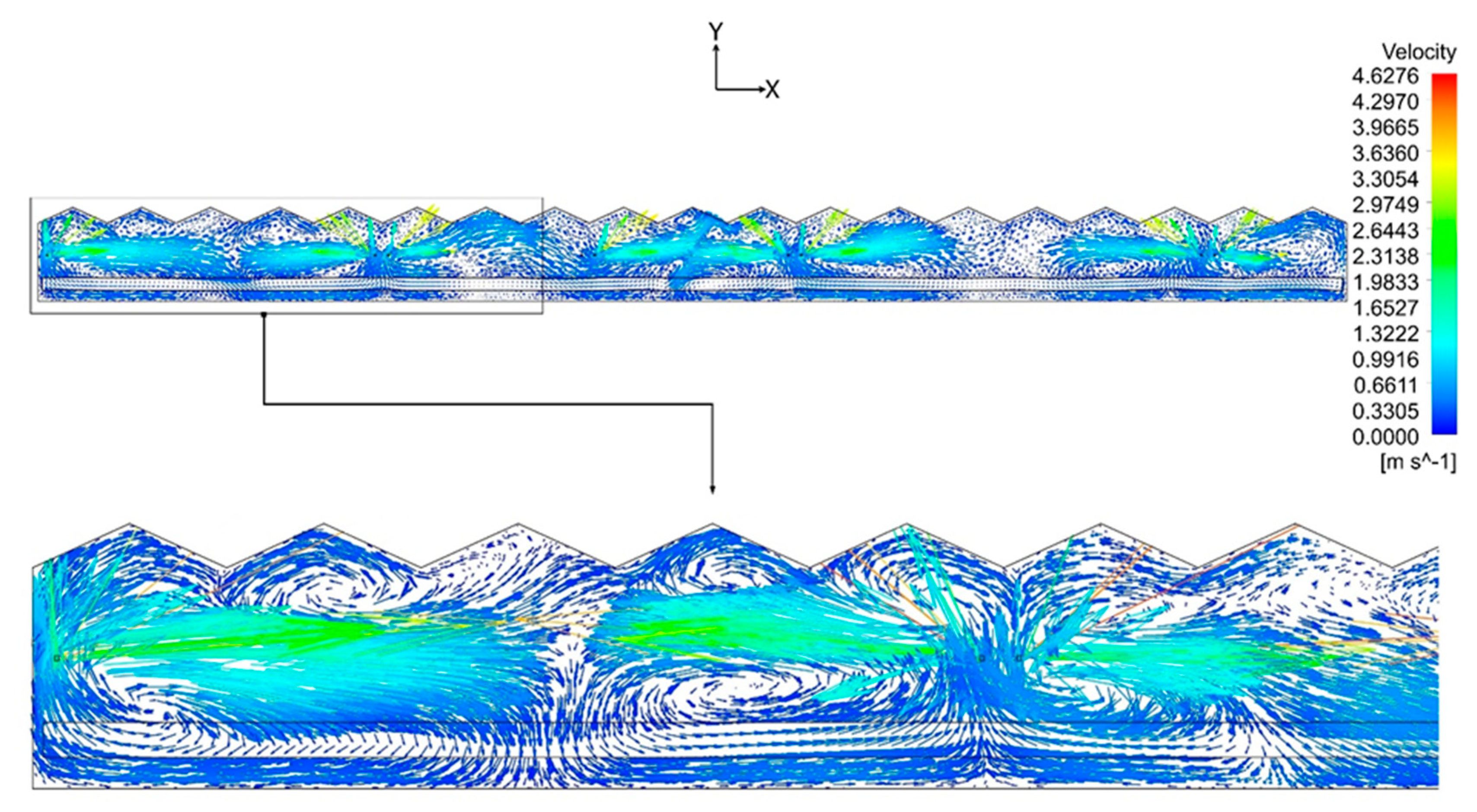
3.2. Airflow Analysis

The measured and simulated vertical air velocity distribution at the eastern, central, and western sections of the greenhouse is graphically represented in Figure 6. The simulated and measured air velocity values were averaged for the 60 min, 300 min, and 480 min periods.

A similar trend was observed between the measured and simulated air speeds, with both decreasing with a decrease in height. Measured air speeds at the eastern and western sections of the greenhouse were on average 17.6% and 29.4%, respectively, lower than the values at the central section. This was mainly attributed to the relative distance of sampling locations to the FCU linear array.

Air velocity within the crop canopy was much lower relative to the inlet velocity, with maximal values of 0.81 ms⁻¹, representing an 83.78% decrease with respect to the inlet velocity. These maximal values were restricted in the regions where the horizontal hot air jet from the FCU came in contact with the crop canopy. The air velocity within most of the canopy ranged from 0.07 ms⁻¹ to 0.61 ms⁻¹. These were average values for the 60 min, 300 min, and 480 min periods. The mean air velocity at the crop level was $0.18{ \mathrm{ms}}^{-1}$.

Air velocity profiles along the longitudinal cross-section at 2.0 m and 2.5 m are as shown in Figure 7. The simulated and measured air velocity values were averaged for the 60 min, 300 min, and 480 min periods.

There was a fair agreement between the measured and simulated values. Significantly higher air velocities were observed at the regions between the FCU linear array as opposed to the other regions inside the greenhouse, as illustrated in Figure 7. This was expected, as the horizontal airflow from the FCUs were directed and concentrated in these regions. This difference in air velocities gave rise to a periodicity in the air velocity profile.

To allow for the visualization of the airflow structure, the velocity vector vertical profiles in the vertical longitudinal mid-plane of the greenhouse were plotted as shown in Figure 8.

Airflow displacements were directed horizontally into the greenhouse from the FCU in the $+X$ or $-X$ direction depending on the orientation of the FCU discharge vent. The general airflow consisted of forced convective air heading towards the crop canopy and the greenhouse roof. A detailed analysis of the airflow pattern showed that convective cells developed above and below the horizontal airflow displacements.

Below the FCUs, due to high airflow velocity from the FCUs, air currents develop rotating concentric convention loops moving through the crop canopy, changing direction upon impinging the greenhouse floor and flowing towards the outlets. The rotating convection loops move in a clockwise direction for horizontal airflow displacement in the $+X$ direction and counterclockwise for the $-X$ airflow displacement. Above the FCUs, air currents flowing towards the roof develop a series of convective air loops within each span of the roof area. These convective air rolls are caused by buoyancy effects whereby hot and low-density air from the FCUs loses its heat when it comes in contact with the cold roof surface and the resulting cold and high-density air flows back towards the FCUs. The direction of rotation of the convective air rolls is in the counterclockwise direction for airflow displacement in the $+X$ direction and clockwise for the $-X$ airflow displacement. This aerodynamic behavior plays an essential role in temperature homogeneity, as a large percentage of the heat is transported by these rotating airflow loops through the greenhouse space. A similar airflow pattern and distribution was reported by Tadj et al. [14] using 3-D ultrasonic anemometers and CFD simulations and by López et al. [38], who investigated airflow structure generated by air heaters using 2-D and 3-D ultrasonic anemometers that were simultaneously moved to 192 locations within a Mediterranean greenhouse.

3.3. Thermal Assessment

Time evolutions of measured and simulated average greenhouse interior air temperature are as shown in Figure 9.

Figure 9 shows a similar trend between the measured and modeled air temperatures. Generally, there was good agreement between the simulated air temperatures and the measured ones, with a mean temperature overestimation of $1.62 ℃$ for the 8 h period considered. There was a steep increase in greenhouse interior temperature from the 60 min to the 300 min period, a consequence of active heating and an increase in both the greenhouse exterior temperature and solar radiation. Maximal measured and predicted air temperatures attained were $22.97 ℃$ and $23.95 ℃$, respectively, equivalent to a $4.28\%$ difference and coinciding with the period that recorded the highest exterior temperature of $8.83 ℃$ and received a maximum solar radiation of $175{ \mathrm{Wm}}^{-2}$, as illustrated in Figure 2. Subsequently, as from the 300 min to the 480 min period, there was a noticeable decrease in air temperature despite active heating. Both the greenhouse outside conditions and solar radiation had a declining trend, explaining this noticeable decrease in greenhouse inside air temperature.

The CFD model slightly overestimated the air temperatures mainly due to air infiltration losses at the joints of the walls, roof, and side windows of the envelope that could not be measured and were thus ignored. The greenhouse was modeled as an airtight model. Thermally-induced infiltration losses resulted from a significant difference between greenhouse interior and exterior air temperature (Figure 2A). Wind-induced infiltration losses caused by high exterior wind speeds that oscillated between $1.44{ \mathrm{ms}}^{-1}~7.13{ \mathrm{ms}}^{-1}$, with hourly average values $\ge 2.5 {\mathrm{ms}}^{-1}$ (Figure 2B), usually lead to a higher air infiltration [40]. Furthermore, air infiltration and leakage ventilation are generally assumed to increase linearly with external wind speed, as was observed by Kuroyanagi [9]. Indeed, air infiltration and its impact on both thermal and energy performance have been extensively studied in greenhouses [9,41,42] and buildings [43].

Temperature profiles along the longitudinal cross-section of the greenhouse for the 60 min, 300 min, and 480 min periods are illustrated in Figure 10.

Figure 10 depicts a satisfactory agreement between the measured and simulated values with no significant longitudinal thermal gradient. A periodicity is observed in the simulated temperature profiles, which was also seen in the longitudinal air velocity profile. Globally, air temperatures are 1 K~1.5 K higher in the regions between the FCU linear array than the regions immediately around it, giving rise to this periodicity in the air temperature profile. This phenomenon is in agreement with the analysis of the airflow pattern, in which higher air velocities also existed in regions between the FCU linear array in contrast to other regions. Despite the periodicity, the air temperature is homogeneous with periodic variations of less than 1.5 K upon exclusion of the boundaries. The simulated temperature was plotted against the horizontal longitudinal plane at the heights of 2.0 m and 2.5 m above the ground to visualize this periodicity and is illustrated in Figure 11.

Figure 12 illustrates simulated and measured vertical profiles of air temperatures at the central location of the greenhouse.

Overall, there was good agreement between the simulations and measurements with no significant vertical thermal gradient. There was a gradual decrease in temperature below and above the FCUs with the highest values registered close to the FCUs and the lowest values near the boundaries.

There was a steady decline in temperature within the crop canopy as hot air gradually lost its heat as it moves through the canopy. Mean measured canopy temperature values at 60 min, 300 min, and 480 min were $18.06 ℃, 21.46 ℃,$ and $21.22 ℃$, respectively, and mean simulated canopy temperature values at 60 min, 300 min, and 480 min were $20.3 ℃, 22.83 ℃$, and $22.63 ℃$, respectively.

The vertical profile of air temperature was illustrated by the temperature distribution contours along the transverse plane of the greenhouse. The contours were plotted for the 60 min, 300 min, and 480 min periods as illustrated in Figure 13.

Temperature contours (Figure 13) revealed homogeneity of temperature within the greenhouse domain with slightly higher temperature concentration patches around the FCUs and low temperatures at the regions adjacent to the boundaries. Temperature gradients existed near the greenhouse roof, walls, and floor, with a homogeneous air temperature distribution in most of the greenhouse space. A similar temperature contour pattern was observed by Dhiman et al. [36].

Temperature heterogeneity within the greenhouse can cause non-uniform crop development [1,44]. As such, there is a need to analyze the spatial distribution of temperature, which is evaluated by computing the thermal gradient $\Delta T$ and its standard deviation ${\sigma }_{SD}$. Thermal gradient describes the temperature difference between the greenhouse interior and exterior environments. $\Delta T$ for the 60 min, 300 min, and 480 min periods is presented in Figure 14.

The mean values of $\Delta T$ for the 60 min, 300 min, and 480 min periods were $6.57 ℃$, $15.13 ℃,$ and $17.83 ℃,$ respectively, with a mean value of $15.5 ℃$ over the 8 h period (See Figure 14). These $\Delta T$ values are similar to those reported by authors who also investigated heated greenhouses. Tadj et al. [14] observed an inside–outside temperature difference of $15 ℃,$ deploying a single air heater in a $160{ \mathrm{m}}^2$ single arch greenhouse. Baille et al. [45] registered a $\Delta T$ value of $14.1 ℃$ in a $432 {\mathrm{m}}^2$ Spanish Parral-type greenhouse by using a single mobile air-convection heating system. López et al. [38], who used a single air heater in a $20\times 24 {\mathrm{m}}^2$3-span arched roof greenhouse, reported a $\Delta T$ value of $11.2 ℃$. Kittas et al. [46] recorded a $\Delta T$ value of $10 ℃$ in a 1-span $31\times 6.5{ \mathrm{m}}^2$ Venlo-type pipe-heated greenhouse.

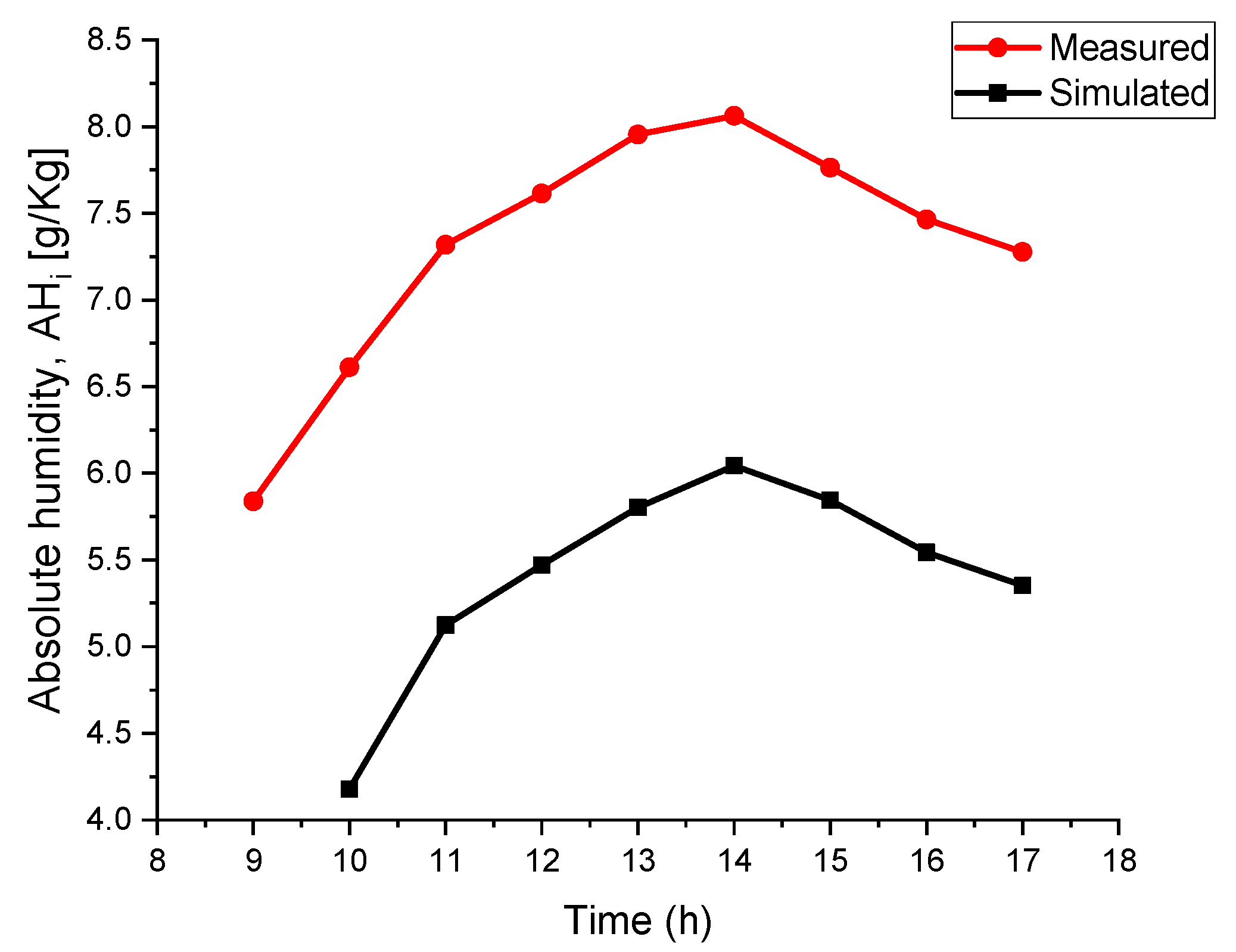
3.4. Humidity Analysis

Time evolutions of the measured and simulated absolute humidity are plotted as shown in Figure 15.

The measured and simulated values exhibited a similar trend, with good agreement between the values as shown in Figure 15. There was a gradual increment in absolute humidity from the 60 min period to the 300 min period, attaining maximal measured and simulated values of $8.06 {\mathrm{g} \mathrm{kg}}^{-1}$ and $6.04 {\mathrm{g} \mathrm{kg}}^{-1}$, respectively. Subsequently, as from the 300 min to the 480 min period, there was a steady decline in absolute humidity. As was expected, the model slightly underestimated absolute humidity by a mean value of $2.08 {\mathrm{g} \mathrm{kg}}^{-1}$ for the 8 h period due to the same reasons that caused thermal overestimation. Similar absolute humidity values were observed by Tadj et al. [14] and Montoya et al. [47].

Simulated and measured vertical profiles of absolute humidity at the central location of the greenhouse are illustrated in Figure 16.

Figure 16 shows a similar trend between the measured and simulated values with no significant vertical gradient of absolute humidity. The agreement between the measured and simulated values was reasonably acceptable. Absolute humidity decreased with an increase in the height, with a sharp decline at FCU height level. This was due to the psychrometric correlation of relative humidity to temperature. Therefore, high temperatures, which were prevalent around the FCU, resulted in lower relative humidity values and lower temperatures resulted in higher relative humidity.

The spatial distribution patterns as described by the absolute humidity transverse contours (Figure 17) further describe the inverse relationship between relative humidity and temperature, with drier regions around the FCUs registering lower values of absolute humidity and regions around the floor and roof recording higher values of absolute humidity, which coincides with observations by Tadj et al. [14].

Absolute humidity profiles along the longitudinal cross-section of the greenhouse for the 60 min, 300 min, and 480 min periods are graphically illustrated in Figure 18.

The agreement between the measured and simulated values was satisfactory, with no strong longitudinal gradient of absolute humidity. The same periodicity that was observed in the air velocity and air temperature profiles can also be seen here, though the cyclic fluctuations are much weaker than those exhibited in air temperature. It is interesting to see that the periodicity peaks of absolute humidity were inverse to those of air temperature due to the inverse relationship of the two variables.

The time evolution of simulated crop transpiration flux $Q_{lat}$ is illustrated in Figure 19.

As illustrated in Figure 19, $Q_{lat}$ increased gradually from 60 min to 300 min to attain a maximal value of $19{ \mathrm{Wm}}^{-2}$, which coincided with the point that received the maximum solar radiation. As from 300 min to 480 min, $Q_{lat}$ decreased with the decline of $R{g}_o$. With no substantial variation in values of $T_i$ and $R{H}_{i }$, $Q_{lat}$ had a strong correlation to solar radiation $R{g}_o$. This transient trend of $Q_{lat}$ is similar to those observed by Ali et al. [32] and Villarreal-Guerrero et al. [34].

4. Discussion

Validation of the numerical simulation is essential before it is applied as an assessment tool to explore the microclimate variables within a greenhouse. Thus, the developed CFD model was validated with experimental data collected in the greenhouse. Vanthoor et al. [48] and Baptista et al. [49] concluded that hourly RMSE air temperature and humidty values of around $10~15\%$ from models that apply climate data are satisfactory and reasonably acceptable for transient simulation. MAE values obtained corresponded to values attained by similar studies that adopted the same methodological approach. Tadj et al. [14] reported MAE values of $16\%$ for air temperature and humidity and $29\%$ for air velocity, while Li et al. [50] obtained mean MAE values of around $15\%$ for air temperature and humidity and around $20\%$ for air velocity. R² values of more than 0.8 were obtained, which depicted the high correlation between the measured and simulated datasets. It is noteworthy that accurate validation of CFD models still remains a problem, especially in a real full-scale greenhouse with difficulty in mapping environmental variables inside the greenhouse [11] and sensor-accuracy limitations [50]. Nevertheless, there was good agreement between the measured and simulated values, and the validation results were satisfactory and suggested a reliable CFD model. Furthermore, the results of the statistical analysis undertaken to evaluate the capability of the CFD model to predict air velocity, temperature, and humidity in the greenhouse showed that there was no significant difference in the measured and simulated datasets, indicating that the developed transient 3-D numerical model could be applied as a tool to evaluate the dynamic thermo-environmental behavior inside the heated Venlo-type greenhouse.

The airflow results were initially analyzed after validation of the model. This allowed for the determination of the one of the established hypotheses, which was to ascertain that the airflow pattern inside the greenhouse influenced the spatial distribution of temperature and humidity as it had been determined in other agricultural buildings [10,14,38,51]. It was observed that the periodicity in the air velocity profile was also replicated in the temperature and humidity profile, ascertaining that the airflow pattern shaped the distribution of temperature and humidity. This coincides with findings by Bournet et al. [51,52] that the thermal and hygrometric performance is strongly influenced by air movement and distribution within the greenhouse interior.

The thermal spatial distribution was shaped by the airflow pattern inside the greenhouse. Homogeneous thermal conditions were observed inside the greenhouse, with the exception of regions near the FCUs and the boundaries, in accordance with conditions observed by Dhiman et al. [36]. Globally, the inside air temperatures attained of between $18.38 ℃$ and $23.95 ℃$ were above the minimum recommended value of $10 ℃$ [53]. This temperature range is favorable for a broad range of crop species, providing suitable thermal conditions that translate to increased crop quality and productivity [54,55]. Further, it was found that crop-zone temperature was lower than the greenhouse inside air. Tadj et al. [14] and Teitel et al. [56] made similar observations, which they concluded was a drawback of employing air heaters. This phenomenon increases the risk of condensation on the leaves that enhances the development of plant diseases such as blight and botrytis. This can be remedied by installing the FCUs at a lower location, leading to a higher temperature within the crop-zone area, but drawbacks of a low installation location are that it would hinder general crop care and the FCUs may need to be chemical resistant. Lastly, the mean value of the thermal differential of $15.5 ℃$ over the 8 h period was consistent with those reported in studies from different regions around the globe that also investigated heated greenhouses [14,38,45,46].

The psychrometric correlation of relative humidity to temperature determined the spatial distribution of relative humidity in that high temperatures resulted in lower relative humidity values and lower temperatures resulted in higher relative humidity, in agreement with what was noted by Bournet et al. [57] and Piscia et al. [58]. The average greenhouse interior measured and simulated relative humidity both went below 50% during the experimentation period, below the recommended value of 65% [59]. This was as a result of a drier climate within the greenhouse caused by the hot air stream discharged by FCUs, which had a significant effect on humidity. Therefore, when air heaters are deployed in greenhouses, it is generally recommended to accompany them with humidification systems, which was not the case with the evaluated greenhouse. Conversely, disease infestations that plague greenhouses due to high humidity are mitigated by these low levels of humidity, subsequently reducing the use of agrochemicals, which is a positive effect on human health and the environment [60,61]. It is held that the ideal relative humidity for favorable plant growth is approximately 80~85% [59], with levels above 85% resulting in restricted transpiration rates, which leads to dehydration and leaf wilting [57]. In contrast, humidity levels of below 40% increase transpiration rate and stomatal resistance, which can cause water stress in inadequate irrigation conditions [62].

Application of a single air heater in the greenhouse, as was undertaken by Tadj et al. [14], López et al. [38], and Baille et al. [45], resulted in considerable temperature heterogeneity with significant longitudinal and vertical thermal gradients due to warm air stagnation in the highest part of the greenhouse. In this study, utilization of multiple FCUs and installation of the FCUs in a linear array with the orientation of the FCU discharge vents facing each other, as shown in Figure 4, enabled hot airflow into the zone between the FCU array from multiple locations. This limited temperature heterogeneity within the greenhouse corroborating the authors’ conclusion that usage of multiple air heaters in the greenhouse would lead to a more homogeneous microclimate.

Finally, this research was a preliminary but fundamental attempt to assess the variable greenhouse microclimate parameters in a heated Venlo-type greenhouse. Nonethesless, this work was not without limitations, which included the challenge of precise CFD model validation, sensor accuracy limitations, and long computation times due to the computationally intensive transient simulations. In future, improvements in numerical model validation techniques will possibly allow for more accurate validation of CFD models, and simulation computing times will gradually reduce as a result of technological advancements in computational performance.

5. Conclusions

The 3-D transient model developed was reliable and enabled the comprehensive evaluation of the spatial and temporal distribution of air velocity, temperature, and humidity in the heated Venlo-type greenhouse. Validation of the model using statistical indices showed good agreement between measured and simulated datasets, with mean hourly air temperature MAE and RMSE values of $7.7\%$ and $7.9\%,$ respectively, and mean hourly air humidity MAE and RMSE values of $16.18\%$ and $16.42\%,$ respectively. The results of the statistical analysis showed no significant difference in the datasets, indicating the capability of the developed numerical model to predict the behavior of microclimate variables inside the heated greenhouse. The CFD model demonstrated that the airflow pattern inside the greenhouse shaped the distribution of temperature and absolute humidity, with the periodicity observed in the air velocity profile replicated in the temperature and humidity profiles. Homogeneity of temperature and humidity was prevalent inside the greenhouse, with no significant longitudinal or vertical gradients of either variable primarily due to the use and installation pattern of multiple FCUs in the greenhouse. It can therefore be concluded that all the chosen research hypotheses were confirmed.

The results obtained in this study can be applied as a foundation for future studies in the Yangtze River Delta region and other sub-tropical climatic regions around the world seeking to provide information that can assist growers to improve crop production and designers to optimize climate control systems by leveraging spatio-temporal 3-D distributed climate inside the greenhouse.

References

1. Odhiambo, M.; Wang, X.; de Antonio, P.; Shi, Y.; Zhao, B. Effects of Root-Zone Temperature on Growth, Chlorophyll Fluorescence Characteristics and Chlorophyll Content of Greenhouse Pepper Plants Grown under Cold Stress in Southern China. Russ. Agric. Sci. 2018, 44, 426–433. [Google Scholar] [CrossRef]
2. Peng, B.; Wang, Y.; Elahi, E.; Wei, G. Behavioral game and simulation analysis of extended producer responsibility system’s implementation under environmental regulations. Environ. Sci. Pollut. Res. 2019, 26, 17644–17654. [Google Scholar] [CrossRef] [PubMed]
3. Elahi, E.; Weijun, C.; Jha, S.K.; Zhang, H. Estimation of realistic renewable and non-renewable energy use targets for livestock production systems utilising an artificial neural network method: A step towards livestock sustainability. Energy 2019, 183, 191–204. [Google Scholar] [CrossRef]
4. Riad, P.; Graefe, S.; Hussein, H.; Buerkert, A. Landscape transformation processes in two large and two small cities in Egypt and Jordan over the last five decades using remote sensing data. Landsc. Urban Plan. 2020, 197, 103766. [Google Scholar] [CrossRef]
5. Benli, H. Energetic performance analysis of a ground-source heat pump system with latent heat storage for a greenhouse heating. Energy Convers. Manag. 2011, 52, 581–589. [Google Scholar] [CrossRef]
6. Kumar, K.V.; Bai, R.K. Solar greenhouse assisted biogas plant in hilly region–A field study. Sol. Energy 2008, 82, 911–917. [Google Scholar] [CrossRef]
7. Esen, M.; Yuksel, T. Experimental evaluation of using various renewable energy sources for heating a greenhouse. Energy Build. 2013, 65, 340–351. [Google Scholar] [CrossRef]
8. Ghoulem, M.; El Moueddeb, K.; Nehdi, E.; Boukhanouf, R.; Calautit, J.K. Greenhouse design and cooling technologies for sustainable food cultivation in hot climates: Review of current practice and future status. Biosyst. Eng. 2019, 183, 121–150. [Google Scholar] [CrossRef]
9. Kuroyanagi, T. Investigating air leakage and wind pressure coefficients of single-span plastic greenhouses using computational fluid dynamics. Biosyst. Eng. 2017, 163, 15–27. [Google Scholar] [CrossRef]
10. Boulard, T.; Roy, J.-C.; Pouillard, J.-B.; Fatnassi, H.; Grisey, A. Modelling of micrometeorology, canopy transpiration and photosynthesis in a closed greenhouse using computational fluid dynamics. Biosyst. Eng. 2017, 158, 110–133. [Google Scholar] [CrossRef]
11. Ali, H.B.; Bournet, P.-E.; Cannavo, P.; Chantoiseau, E. Using CFD to improve the irrigation strategy for growing ornamental plants inside a greenhouse. Biosyst. Eng. 2019, 186, 130–145. [Google Scholar]
12. Bartzanas, T.; Tchamitchian, M.; Kittas, C. Influence of the heating method on greenhouse microclimate and energy consumption. Biosyst. Eng. 2005, 91, 487–499. [Google Scholar] [CrossRef]
13. Teitel, M.; Barak, M.; Antler, A. Effect of cyclic heating and a thermal screen on the nocturnal heat loss and microclimate of a greenhouse. Biosyst. Eng. 2009, 102, 162–170. [Google Scholar] [CrossRef]
14. Tadj, N.; Bartzanas, T.; Fidaros, D.; Draoui, B.; Kittas, C. Influence of heating system on greenhouse microclimate distribution. Trans. ASABE 2010, 53, 225–238. [Google Scholar] [CrossRef]
15. Couto, N.; Rouboa, A.; Monteiro, E.; Viera, J. Computational fluid dynamics analysis of greenhouses with artificial heat tube. World J. Mech. 2012, 2, 181–187. [Google Scholar] [CrossRef] [Green Version]
16. Flores-Velázquez, J.; Villarreal-Guerrero, F.; Rojano-Aguilar, A.; Schdmith, U. CFD to analyze energy exchange by convection in a closed greenhouse with a pipe heating system. Acta Univ. 2019, 29, e2112. [Google Scholar] [CrossRef]
17. Zeroual, S.; Bougoul, S.; Benmoussa, H. Effect of Radiative Heat Transfer and Boundary Conditions on the Airflow and Temperature Distribution Inside a Heated Tunnel Greenhouse. J. Appl. Mech. Tech. Phys. 2018, 59, 1008–1014. [Google Scholar] [CrossRef]
18. Nebbali, R.; Roy, J.; Boulard, T. Dynamic simulation of the distributed radiative and convective climate within a cropped greenhouse. Renew. Energy 2012, 43, 111–129. [Google Scholar] [CrossRef]
19. Villagrán, E.A.; Romero, E.J.B.; Bojacá, C.R. Transient CFD analysis of the natural ventilation of three types of greenhouses used for agricultural production in a tropical mountain climate. Biosyst. Eng. 2019, 188, 288–304. [Google Scholar] [CrossRef]
20. Tong, G.; Christopher, D.; Li, B. Numerical modelling of temperature variations in a Chinese solar greenhouse. Comput. Electron. Agric. 2009, 68, 129–139. [Google Scholar] [CrossRef]
21. Fidaros, D.; Baxevanou, C.; Bartzanas, T.; Kittas, C. Numerical simulation of thermal behavior of a ventilated arc greenhouse during a solar day. Renew. Energy 2010, 35, 1380–1386. [Google Scholar] [CrossRef]
22. Lam, C.; Bremhorst, K. A modified form of the k-ε model for predicting wall turbulence. J. Fluids Eng. 1981, 103, 456–460. [Google Scholar] [CrossRef]
23. Patel, V.C.; Rodi, W.; Scheuerer, G. Turbulence models for near-wall and low Reynolds number flows—A review. AIAA J. 1985, 23, 1308–1319. [Google Scholar] [CrossRef]
24. Hoff, S.J.; Janni, K.A.; Jacobson, L.D. Three-dimensional buoyant turbulent flows in a scaled model, slot-ventilated, livestock confinement facility. Trans. ASAE 1992, 35, 671–686. [Google Scholar] [CrossRef]
25. Chen, Q. Prediction of buoyant, turbulent Flow by a low-renolds-number k-ε model. ASHRAE Trans. 1990, 96, 564–573. [Google Scholar]
26. Modest, M.F.; Haworth, D.C. Radiative Heat Transfer in Turbulent Combustion Systems: Theory and Applications; Springer: Berlin/Heidelberg, Germany, 2016. [Google Scholar]
27. Versteeg, H.; Malalasekera, W. Computational fluid dynamics. In The Finite Volume Method; Longman Scientific & Technical, Longman Group Limited: London, UK, 1995. [Google Scholar]
28. ANSYS_Inc. ANSYS Fluent 2020 R1 Theory Guide; ANSYS_Inc.: Canonsburg, PA, USA, 2020. [Google Scholar]
29. Haxaire, R. Caractérisation et Modélisation des écoulements d’air Dans une Serre. Ph.D. Thesis, Université de Nice Sophia Antipolis, Nice, France, 1999; pp. 1–148. [Google Scholar]
30. Sase, S.; Kacira, M.; Boulard, T.; Okushima, L. Wind tunnel measurement of aerodynamic properties of a tomato canopy. Trans. ASABE 2012, 55, 1921–1927. [Google Scholar] [CrossRef]
31. Wilson, J.D. Numerical studies of flow through a windbreak. J. Wind Eng. Ind. Aerodyn. 1985, 21, 119–154. [Google Scholar] [CrossRef]
32. Ali, H.B.; Bournet, P.-E.; Cannavo, P.; Chantoiseau, E. Development of a CFD crop submodel for simulating microclimate and transpiration of ornamental plants grown in a greenhouse under water restriction. J. Comput. Electron. Agric. 2018, 149, 26–40. [Google Scholar]
33. Stanghellini, C. Transpiration of Greenhouse Crops. An Aid to Climate Management. Ph.D. Thesis, Wageningen Agricultural University, Wageningen, The Netherlands, 1987. [Google Scholar]
34. Villarreal-Guerrero, F.; Kacira, M.; Fitz-Rodríguez, E.; Kubota, C.; Giacomelli, G.A.; Linker, R.; Arbel, A. Comparison of three evapotranspiration models for a greenhouse cooling strategy with natural ventilation and variable high pressure fogging. Sci. Hortic. 2012, 134, 210–221. [Google Scholar] [CrossRef]
35. Duffie, J.A.; Beckman, W.A. Solar Engineering of Thermal Processes, 4th ed.; John Wiley & Sons: Hoboken, NJ, USA, 2013. [Google Scholar]
36. Dhiman, M.; Sethi, V.; Singh, B.; Sharma, A. CFD analysis of greenhouse heating using flue gas and hot water heat sink pipe networks. Comput. Electron. Agric. 2019, 163, 104853. [Google Scholar] [CrossRef]
37. Duffie, J.A.; Beckman, W.A. Solar Engineering of Thermal Processes, 2nd ed.; John Wiley & Sons: Hoboken, NJ, USA, 1991. [Google Scholar]
38. López, A.; Valera, D.L.; Molina-Aiz, F.; Peña, A. Thermography and sonic anemometry to analyze air heaters in mediterranean greenhouses. Sensors 2012, 12, 13852–13870. [Google Scholar] [CrossRef] [PubMed] [Green Version]
39. Elahi, E.; Abid, M.; Zhang, H.; Cui, W.; Hasson, S.U. Domestic water buffaloes: Access to surface water, disease prevalence and associated economic losses. Prev. Vet. Med. 2018, 154, 102–112. [Google Scholar] [CrossRef] [PubMed]
40. Piscia, D.; Montero, J.I.; Baeza, E.; Bailey, B.J. A CFD greenhouse night-time condensation model. Biosyst. Eng. 2012, 111, 141–154. [Google Scholar] [CrossRef]
41. Semple, L.; Carriveau, R.; Ting, D.S.K. Assessing heating and cooling demands of closed greenhouse systems in a cold climate. Int. J. Energy Res. 2017, 41, 1903–1913. [Google Scholar] [CrossRef]
42. López, J.; Pérez, J.; Montero, J.; Antón, A. Air Infiltration Rate of Almeria “Parral¿ Type” Greenhouse. In Proceedings of the V International Symposium on Protected Cultivation in Mild Winter Climates: Current Trends for Suistainable Technologies 559, Cartagena-Almería, Spain, 7–11 March 2020; pp. 229–232. [Google Scholar]
43. Feijó-Muñoz, J.; González-Lezcano, R.A.; Poza-Casado, I.; Padilla-Marcos, M.Á.; Meiss, A. Airtightness of residential buildings in the Continental area of Spain. Build. Environ. 2019, 148, 299–308. [Google Scholar] [CrossRef]
44. Sauser, B.J.; Giacomelli, D.G.A.; Janes, D.H.W. Modeling the Effects of Air Temperature Perturbations for Control of Tomato Plant Development. Acta Hortic. 1998, 456, 87–92. [Google Scholar] [CrossRef]
45. Baille, A.; López, J.; Bonachela, S.; González-Real, M.; Montero, J. Night energy balance in a heated low-cost plastic greenhouse. Agric. For. Meteorol. 2006, 137, 107–118. [Google Scholar] [CrossRef]
46. Kittas, C.; Katsoulas, N.; Baille, A. Influence of an aluminized thermal screen on greenhouse microclimate and canopy energy balance. Trans. ASAE 2003, 46, 1653. [Google Scholar] [CrossRef]
47. Montoya, A.; Guzmán, J.L.; Rodríguez, F.; Sánchez-Molina, J.A. A hybrid-controlled approach for maintaining nocturnal greenhouse temperature: Simulation study. Comput. Electron. Agric. 2016, 123, 116–124. [Google Scholar] [CrossRef]
48. Vanthoor, B.; Stanghellini, C.; Van Henten, E.J.; De Visser, P. A methodology for model-based greenhouse design: Part 1, a greenhouse climate model for a broad range of designs and climates. Biosyst. Eng. 2011, 110, 363–377. [Google Scholar] [CrossRef]
49. Baptista, F. Modelling the Climate in Unheated Tomato Greenhouses and Predicting Botrytis Cinerea Infection. Ph.D. Thesis, University of Évora, Évora, Portugal, 2007. [Google Scholar]
50. Li, K.; Xue, W.; Mao, H.; Chen, X.; Jiang, H.; Tan, G. Optimizing the 3D Distributed Climate inside Greenhouses Using Multi-Objective Optimization Algorithms and Computer Fluid Dynamics. Energies 2019, 12, 2873. [Google Scholar] [CrossRef] [Green Version]
51. Bournet, P.; Khaoua, S.O.; Boulard, T. Numerical prediction of the effect of vent arrangements on the ventilation and energy transfer in a multi-span glasshouse using a bi-band radiation model. Biosyst. Eng. 2007, 98, 224–234. [Google Scholar] [CrossRef]
52. Bournet, P.-E.; Boulard, T. Effect of ventilator configuration on the distributed climate of greenhouses: A review of experimental and CFD studies. Comput. Electron. Agric. 2010, 74, 195–217. [Google Scholar] [CrossRef]
53. ASAE. Heating, Ventilating and Cooling Greenhouses; American Society of Agricultural Engineers (ASAE): St. Joseph, MI, USA, 2008. [Google Scholar]
54. Abbas, A.; Minli, Y.; Elahi, E.; Yousaf, K.; Ahmad, R.; Iqbal, T. Quantification of mechanization index and its impact on crop productivity and socioeconomic factors. Int. Agric. Eng. J. 2017, 26, 49–54. [Google Scholar]
55. Elahi, E.; Khalid, Z.; Weijun, C.; Zhang, H. The public policy of agricultural land allotment to agrarians and its impact on crop productivity in Punjab province of Pakistan. Land Use Policy 2020, 90, 104324. [Google Scholar] [CrossRef]
56. Teitel, M.; Segal, I.; Shklyar, A.; Barak, M. A comparison between pipe and air heating methods for greenhouses. J. Agric. Eng. Res. 1999, 72, 259–273. [Google Scholar] [CrossRef]
57. Bournet, P.-E. Assessing greenhouse climate using CFD: A focus on air humidity issues. In Proceedings of the International Symposium on New Technologies for Environment Control, Energy-Saving and Crop Production in Greenhouse and Plant 1037, Jeju, Korea, 6–11 October 2013; pp. 971–985. [Google Scholar]
58. Piscia, D.; Muñoz, P.; Panadès, C.; Montero, J. A method of coupling CFD and energy balance simulations to study humidity control in unheated greenhouses. Comput. Electron. Agric. 2015, 115, 129–141. [Google Scholar] [CrossRef]
59. Vadiee, A.; Martin, V. Energy management in horticultural applications through the closed greenhouse concept, state of the art. Renew. Sustain. Energy Rev. 2012, 16, 5087–5100. [Google Scholar] [CrossRef]
60. Elahi, E.; Weijun, C.; Zhang, H.; Nazeer, M. Agricultural intensification and damages to human health in relation to agrochemicals: Application of artificial intelligence. Land Use Policy 2019, 83, 461–474. [Google Scholar] [CrossRef]
61. Elahi, E.; Weijun, C.; Zhang, H.; Abid, M. Use of artificial neural networks to rescue agrochemical-based health hazards: A resource optimisation method for cleaner crop production. J. Clean. Prod. 2019, 238, 117900. [Google Scholar] [CrossRef]
62. Rabbi, B.; Chen, Z.-H.; Sethuvenkatraman, S. Protected cropping in warm climates: A review of humidity control and cooling methods. Energies 2019, 12, 2737. [Google Scholar] [CrossRef] [Green Version]
Figure 1. Variation of mesh elements with simulated average greenhouse interior air temperature.
Sustainability 12 10412 g001
Figure 2. Time evolution of the boundary conditions for the greenhouse: (A) exterior temperature T o and (B) solar radiation R g o and exterior wind speed U o .
Sustainability 12 10412 g002
Figure 3. Simulated air temperatures at (A) 2.0 m and (B) 2.5 m for the 10 s, 30 s, and 60 s time steps.
Sustainability 12 10412 g003
Figure 4. Greenhouse dimensions and layout of the fan coil units (FCUs).
Sustainability 12 10412 g004
Figure 5. Schematic of (A) aerial and (B) transverse view of the layout of the sensors inside the greenhouse.
Sustainability 12 10412 g005
Figure 6. Simulated vertical air speed distribution profiles at the (A) eastern, (B) central, and (C) western sections of the greenhouse together with measured values at 1.1 m, 2.0 m, and 2.5 m.
Sustainability 12 10412 g006aSustainability 12 10412 g006b
Figure 7. Simulated horizontal air speed distribution profile along the longitudinal cross-section together with measured values at 2.0 m and 2.5 m.
Sustainability 12 10412 g007
Figure 8. Air velocity vectors along the longitudinal plane at 300 min.
Sustainability 12 10412 g008
Figure 9. Time evolutions of average greenhouse interior air temperature, T i .
Sustainability 12 10412 g009
Figure 10. Simulated and measured temperature profiles along the greenhouse longitudinal cross-section for the 60 min, 300 min, and 480 min periods.
Sustainability 12 10412 g010
Figure 11. Variation of simulated temperature along the longitudinal planes at (A) 2.0 m and (B) 2.5 m above the floor at 300 min.
Sustainability 12 10412 g011
Figure 12. Modeled vertical profile of air temperature at the central location of the greenhouse together with measured values at 1.1 m, 2.0 m, and 2.5 m and floor temperature.
Sustainability 12 10412 g012
Figure 13. No heatings (A); Temperature contours along the transverse plane of the greenhouse for the (B) 60 min, (C) 300 min, and (D) 480 min periods.
Sustainability 12 10412 g013aSustainability 12 10412 g013b
Figure 14. The simulated thermal differential Δ T for the (A) 60 min, (B) 300 min, and (C) 480 min periods.
Sustainability 12 10412 g014aSustainability 12 10412 g014b
Figure 15. Time evolutions of the measured and simulated absolute humidity, A H i .
Sustainability 12 10412 g015
Figure 16. Modeled vertical profile of absolute humidity at the central location of the greenhouse together with measured values at 2.0 m and 2.5 m.
Sustainability 12 10412 g016
Figure 17. Transverse contours of H2O mass fractions at the central location of the greenhouse. (A) 60 min; (B) 300 min; (C) 480 min.
Sustainability 12 10412 g017
Figure 18. Simulated and measured absolute humidity profiles along the greenhouse longitudinal cross-section for the (A) 60 min, (B) 300 min, and (C) 480 min periods.
Sustainability 12 10412 g018
Figure 19. Time evolutions of simulated transpiration flux Q l a t .
Sustainability 12 10412 g019