Article

Enhancing Small Moving Target Detection Performance in Low-Quality and Long-Range Infrared Videos Using Optical Flow Techniques

Applied Research LLC, Rockville, MD 20850, USA
*
Author to whom correspondence should be addressed.
Remote Sens. 2020, 12(24), 4024; https://doi.org/10.3390/rs12244024
Submission received: 17 November 2020 / Revised: 7 December 2020 / Accepted: 8 December 2020 / Published: 9 December 2020
(This article belongs to the Section Remote Sensing Image Processing)

Abstract

:
The detection of small moving objects in long-range infrared videos is challenging due to background clutter, air turbulence, and small target size. In this paper, we summarize the investigation of efficient ways to enhance the performance of small target detection in long-range and low-quality infrared videos containing moving objects. In particular, we focus on unsupervised, modular, flexible, and efficient methods for target detection performance enhancement using motion information extracted from optical flow methods. Three well-known optical flow methods were studied. It was found that optical flow methods need to be combined with contrast enhancement, connected component analysis, and target association in order to be effective for target detection. Extensive experiments using long-range mid-wave infrared (MWIR) videos from the Defense Systems Information Analysis Center (DSIAC) dataset clearly demonstrated the efficacy of our proposed approach.

Graphical Abstract

1. Introduction

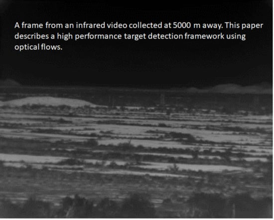
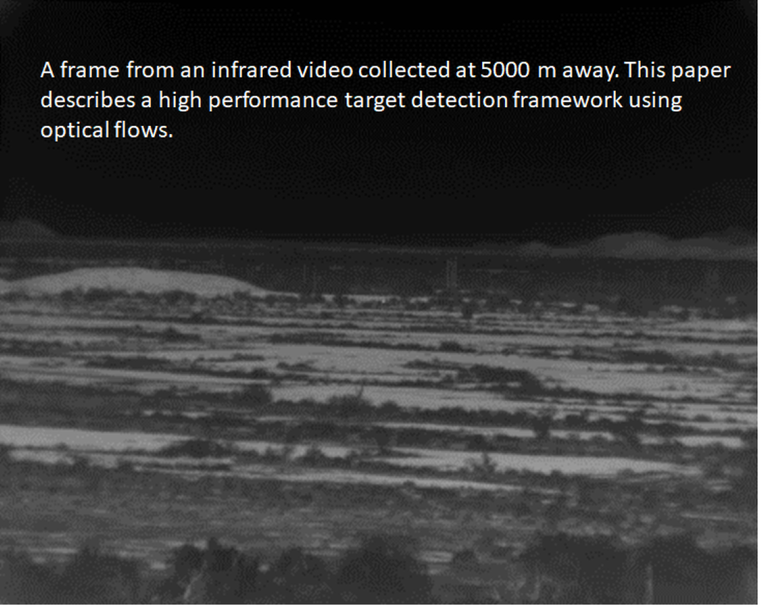
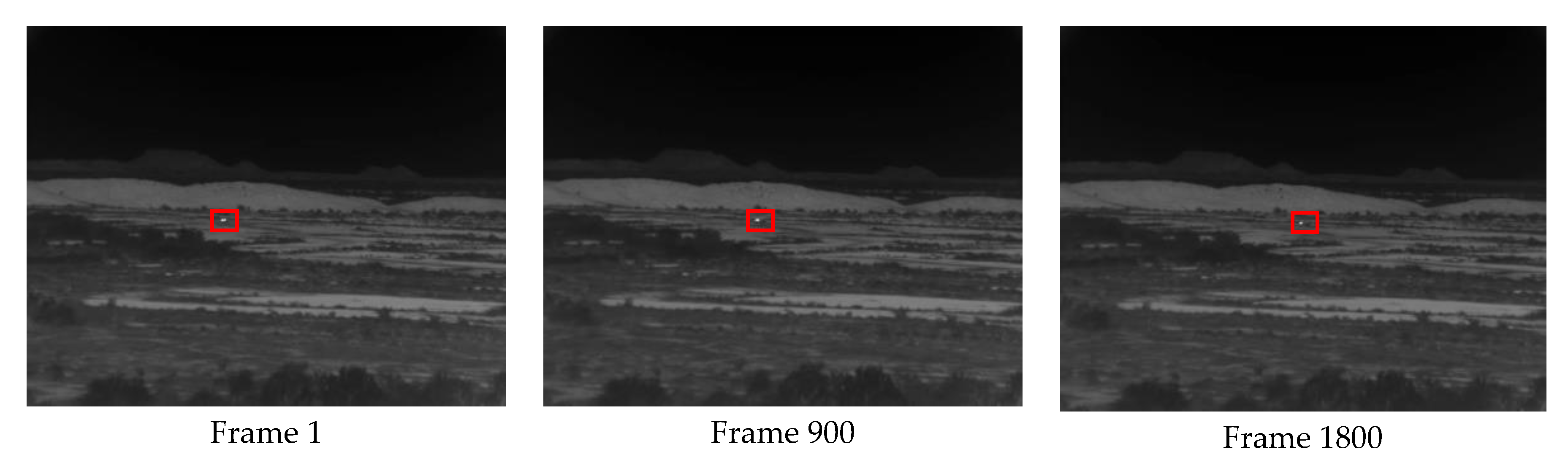
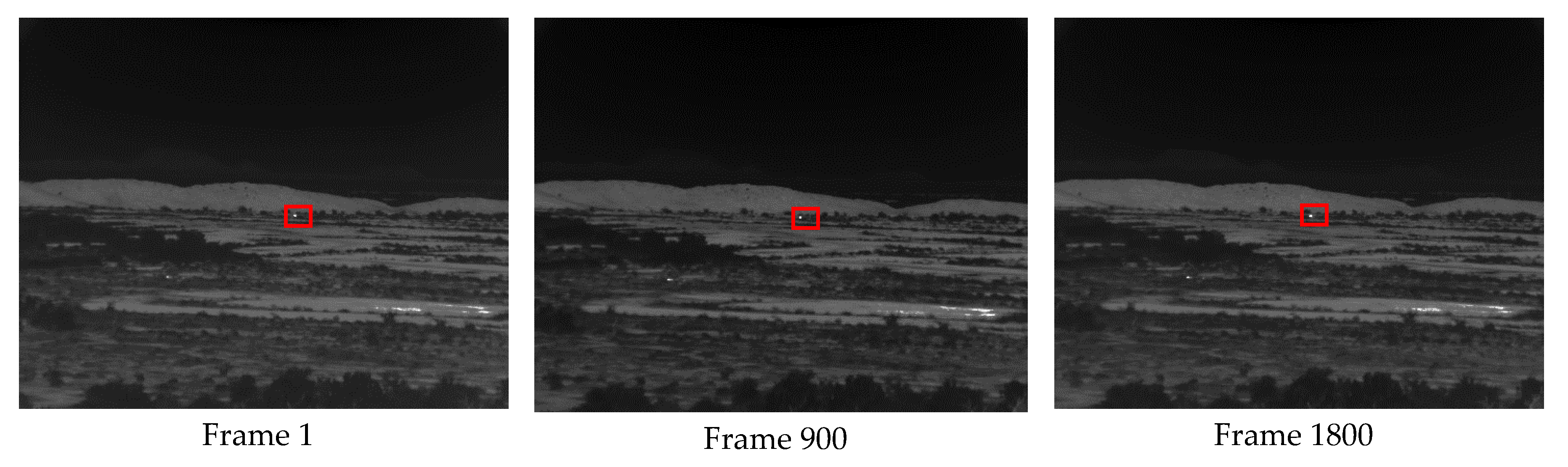
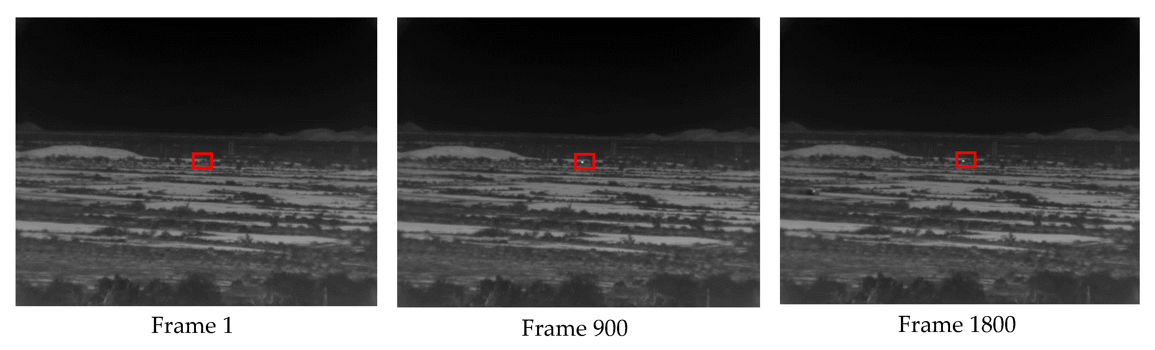
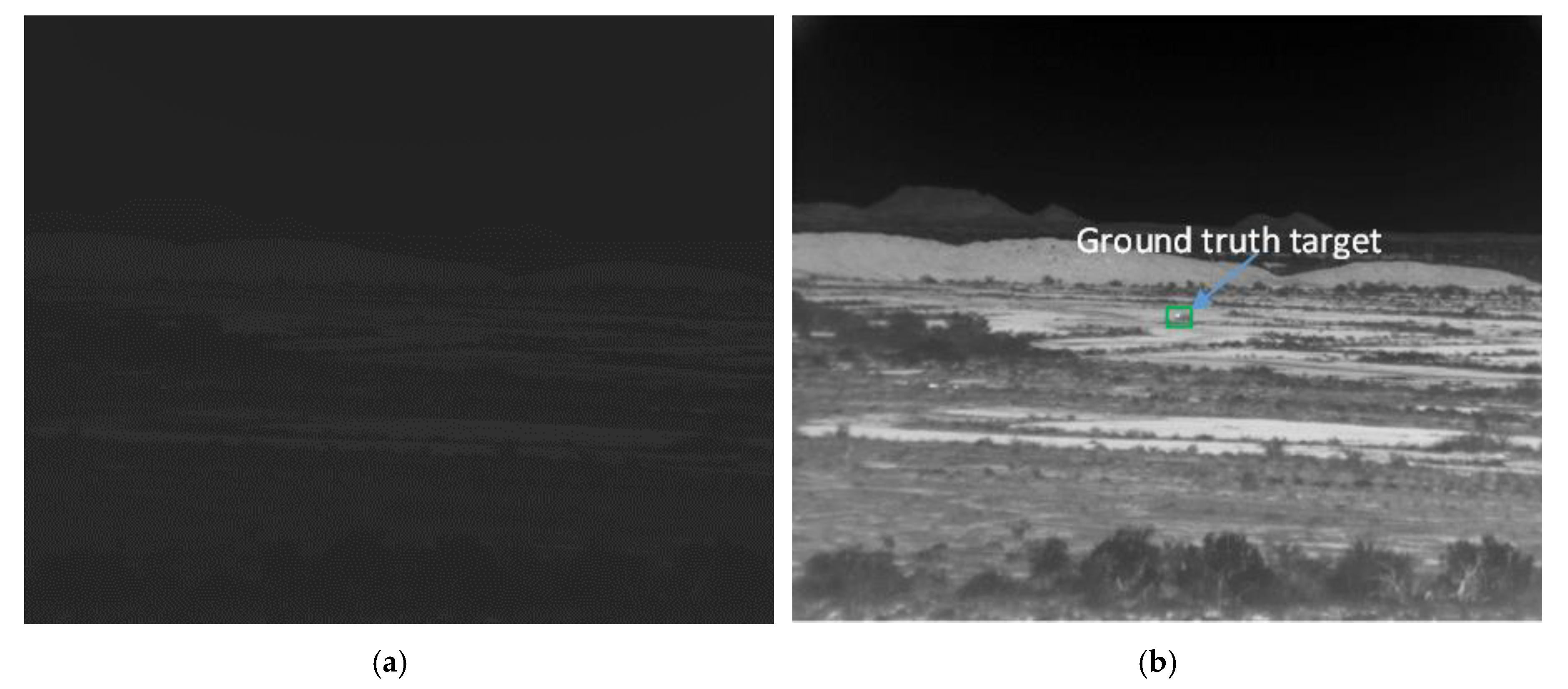
Infrared videos in ground-based imagers contain a lot of background clutter and flickering noise due to air turbulence, sensor noise, etc. Moreover, the target size in long-range videos is quite small and hence it is challenging to detect small targets from a long distance. Furthermore, the contrast is also poor in many infrared videos.
There are two groups of target detection algorithms for videos. One group is to utilize supervised learning algorithms. For instance, there are some conventional target tracking methods [1,2]. In addition, some target detection and classification schemes using deep learning algorithms such as You Only Look Once (YOLO) for larger objects in short-range optical and infrared videos have been proposed in the literature [3,4,5,6,7,8,9,10,11,12,13,14,15,16,17,18,19,20,21]. There are also some recent papers on moving target detection in thermal imagers [22,23,24]. Training videos are required in these algorithms. Although the performance is reasonable for short ranges up to 2000 m in some videos, the performance dropped quite considerably in long ranges where the target sizes are so small. This is because YOLO uses texture information to help the detection. Moreover, the object sizes need to be large enough in order to have textures. The use of YOLO is not very effective for long-range videos in which the targets are too small to have any discernible textures. Some recent algorithms [3,4,5,6,7,8,9,10,11,12,13] incorporated compressive measurements directly for detection and classification. Real-time issues have been discussed in [21].
Another group belongs to the unsupervised approach, which does not require any training data. The latter group is more suitable for long-range videos in which the object size is very small. Chen et al. [25] proposed to detect small IR targets by using local contrast measure (LCM), which is time-consuming and sometimes enhances both targets and clutters. To improve the performance of LCM, Wei et al. [26] introduced a multiscale patch-based contrast measure (MPCM). Gao et al. [27] developed an infrared patch-image (IPI) model to convert small target detection to an optimization problem. Zhang et al. [28] improved the performance of the IPI via non-convex rank approximation minimization (NRAM). Zhang et al. [29] proposed to detect small infrared (IR) targets based on local intensity and gradient (LIG) properties, which has good performance and relatively low computational complexity.
In a recent paper by us [30], we proposed a high-performance and unsupervised approach for long-range infrared videos in which the object detection only used one frame at a time. Although the method in [30] is applicable to both stationary and moving targets, the computational efficiency is not suitable for real-time applications. Since some long-range videos only contain moving objects, it will be good to devise efficient algorithms that can utilize motion information for object detection.
In this paper, we propose an unsupervised, modular, flexible, and efficient framework for small moving target detection in long-range infrared videos containing moving targets. One key component is the use of optical flow techniques for moving object detection. Three well-known optical flow techniques, including Lucas–Kanade (LK) [31], Total Variation with L1 constraint (TV-L1) [32], and (Brox) [33], were compared. Another component is to use object association techniques to help eliminate false positives. It was found that optical flow methods need to be combined with contrast enhancement, connected component analysis, and target association in order to be effective. Extensive experiments using long-range mid-wave infrared (MWIR) videos from the Defense Systems Information Analysis Center (DSIAC) dataset [34] clearly demonstrated the efficacy of our proposed approach.
The contributions of our paper are summarized as follows:
  • We proposed an unsupervised small moving target detection framework that does not require training data. This is more practical as compared to deep-learning-based methods, which require training data and larger object size.
  • Our framework incorporates optical flow techniques that are more efficient than other methods such as [30].
  • Our framework is applicable to long-range and low-quality infrared videos that are beyond 3000 m.
  • We compared several contrast enhancement methods and demonstrated the importance of contrast enhancement in small target detection.
  • Our framework is modular and flexible in that newer methods can be used to replace old methods.
Our paper is organized as follows. Section 2 summarizes the optical flow methods and the proposed framework. Section 3 summarizes the extensive experimental results using actual DSIAC videos. Section 4 includes a few concluding remarks and future directions. In the Appendix A, we include some detailed comparisons of several contrast enhancement techniques to improve the raw video quality. Experiments were used to demonstrate which image enhancement method is better from the perspective of target detection.

2. Small Target Detection Based on Optical Flows

In our earlier paper [30], the LIG algorithm only incorporates intensity and gradient information in a single frame. In some videos such as the DSIAC dataset, the targets are actually moving. In this paper, we focus on applying optical flow techniques by exploiting some motion information to enhance the target detection performance.

2.1. Optical Flow Methods

In this section, we briefly introduce three optical flow techniques to extract motion information in the videos.

2.1.1. Lucas–Kanade (LK) Algorithm

The LK algorithm [31] is very simple. A sliding window (3 × 3 or bigger) scans through a pair of images. For each window, the grey value constancy assumption is applied. A set of linear equations is then obtained. A least square solution can then be used to solve for the motion vectors in that window. The process repeats for the whole image.

2.1.2. Total Variation with L1 Constraint (TV-L1)

One problem with the LK algorithm is that it may not perform well for noisy images. The TV-L1 algorithm [32] considers more assumptions, including smoothness and gradient constancy. Moreover, the L1 regularization is used instead of the L2 regularization.
We first experimented with a TV-L1 implementation [35]. However, the results did not correspond well with [32]. More specifically, several key design parameters, such as the lambda, were not adjustable within this implementation. We found a better implementation directly from the authors of [32] and incorporated it into a more robust Python-based workflow that is further discussed in Section 2.3 and Section 2.4.

2.1.3. High Accuracy Optical Flow Estimation Based on a Theory for Warping (Brox)

Similar to TV-L1, the Brox model [33] considers the assumption of smoothness, gradient, and grey value constancy. These were used in conjunction with a spatio-temporal total variation regularizer.

2.2. LK Results

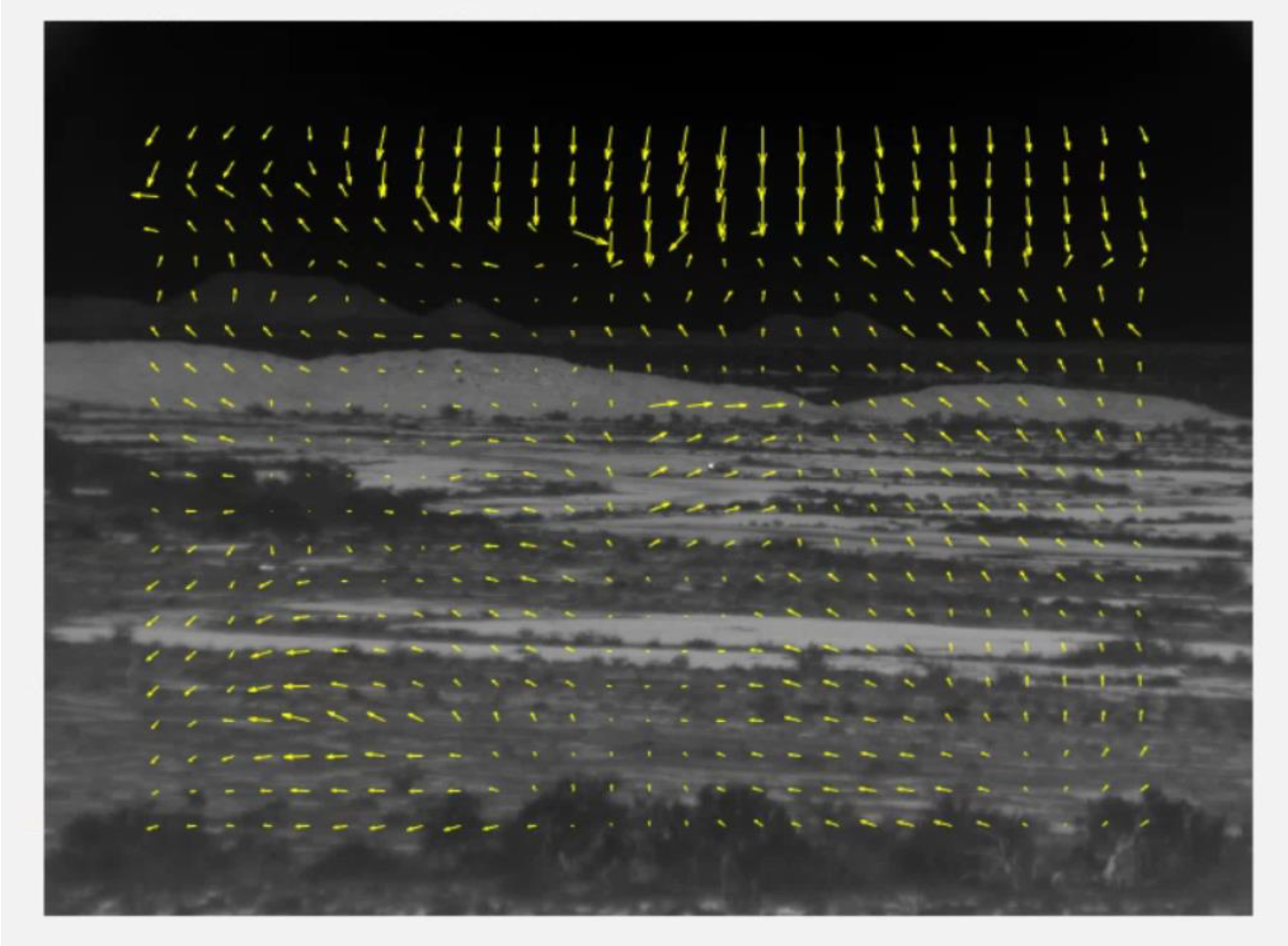
LK is a more traditional optical flow approach. Here, our objective is to see whether or not it would be effective at identifying the location of the target vehicles. The LK method had very poor results for the DSIAC MWIR videos. The motion vectors generated by the LK method show heavy motion outside of the target region, especially in the sky. Figure 1 shows a sample output motion vector fields generated by LK. One can see that the motion vectors have diverse variations and it is difficult to pinpoint where the vehicle is. Although this is a single frame, we found that most optical flow outputs looked similar.
Because of the poor results of LK, we have focused on using TV-L1 and Brox methods in our experiments.

2.3. Proposed Unsupervised Target Detection Architecture for Long-Range Infrared Videos

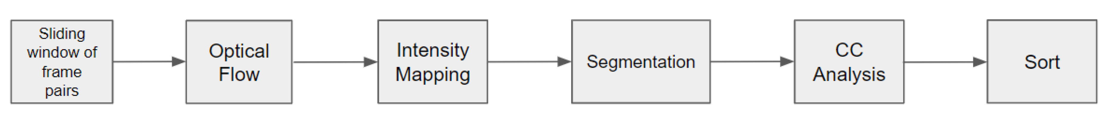
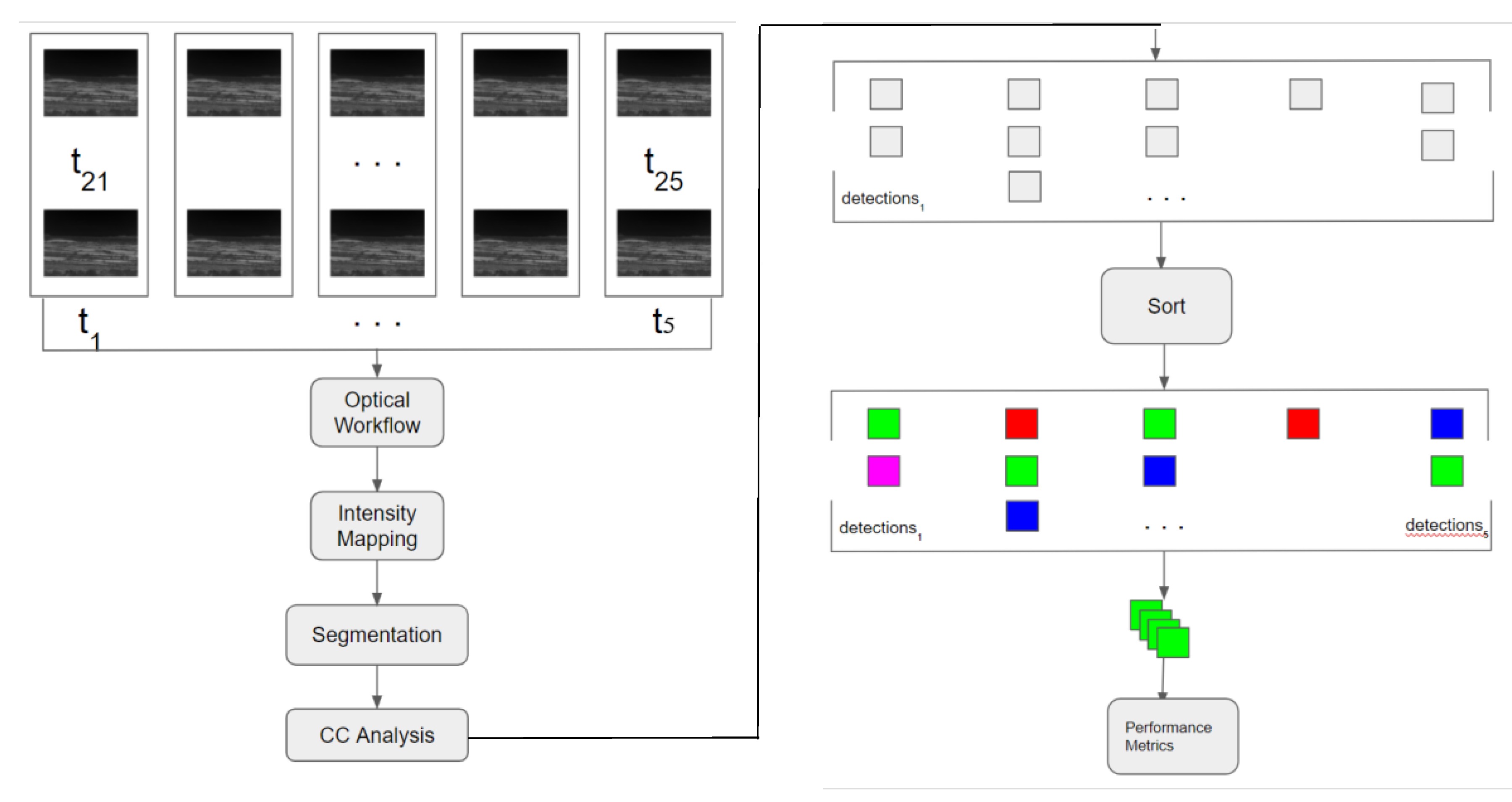
The proposed unsupervised, modular, flexible, and efficient work flow was implemented in Python and is shown in 
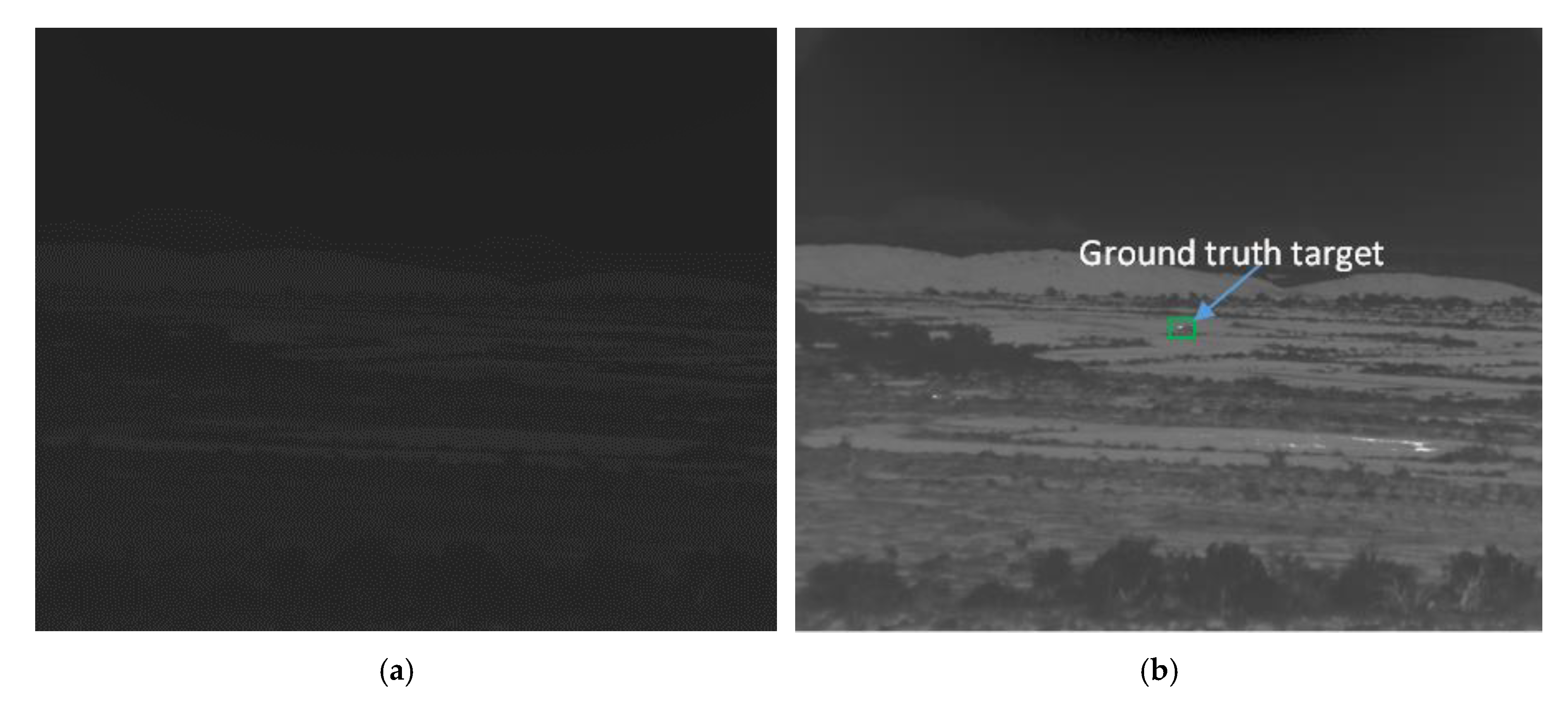
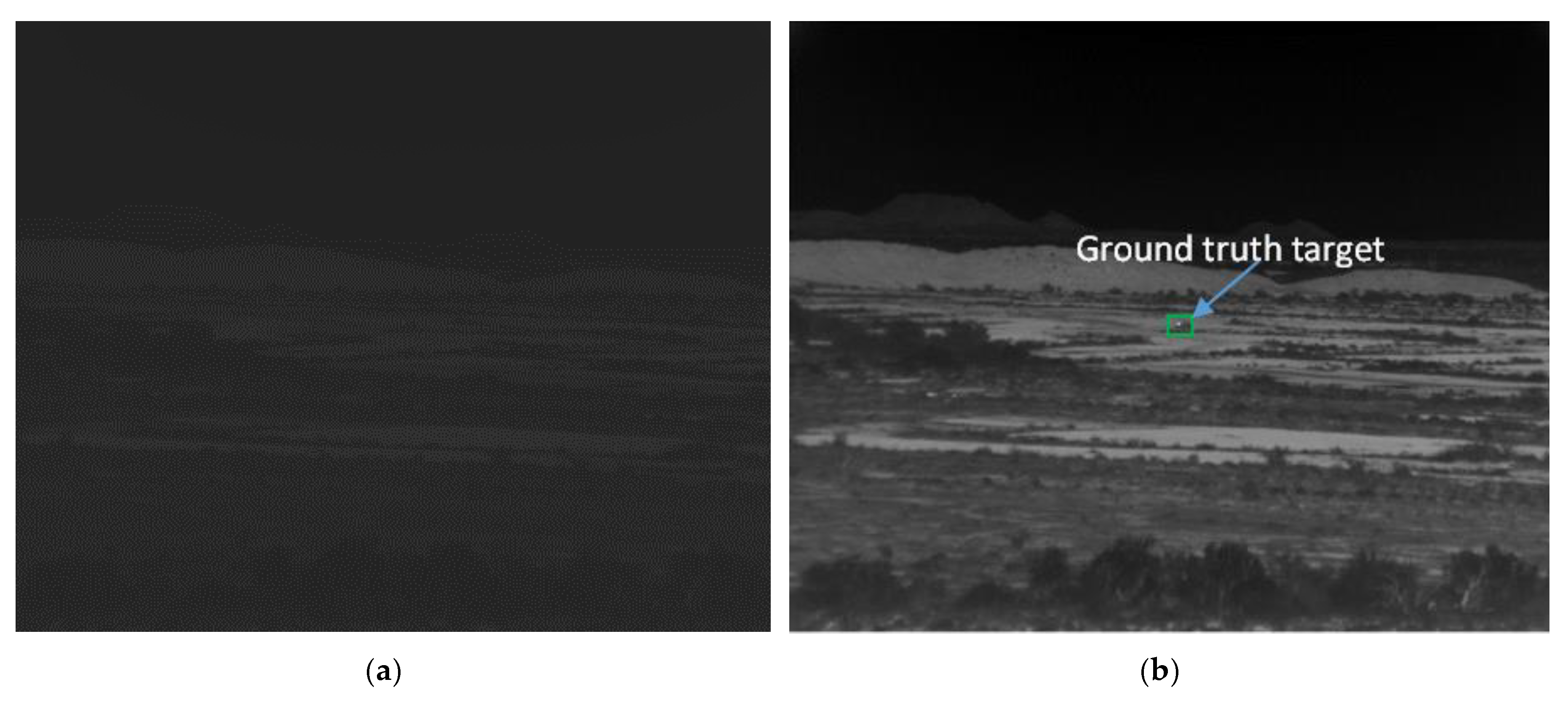
Figure 2. It should be emphasized that the raw video quality in DSIAC videos is poor and contrast enhancement is critical for optical flow methods. In the Appendix A, we include a comparative study of some simple and effective enhancement methods to generate high-quality videos out of the raw videos. There are a number of steps in the proposed workflow. First, frame pairs are selected. In our experiments, the two frames are separated by 19 frames. This was done in order to increase the motion of the target. If adjacent frames are used, the motion in the DSIAC dataset is too subtle to notice. Second, optical flow algorithms are used to the frame pairs to extract the motion vectors. In our experiments, we have compared two algorithms: TV-L1 [32] and Brox [33]. Third, the intensity of the optical flow vectors is computed and used for determining moving pixels. Fourth, the intensity of the optical flow is thresholded based on the mean and standard deviation of the flow intensity. Fifth, a connected component (CC) analysis is performed to the segmented image. Finally, the detected areas are jointly analyzed using a Simple Online and Real-time Tracking (SORT) algorithm [36]. Details of each step are shown below.
Step 1:
Preprocessing
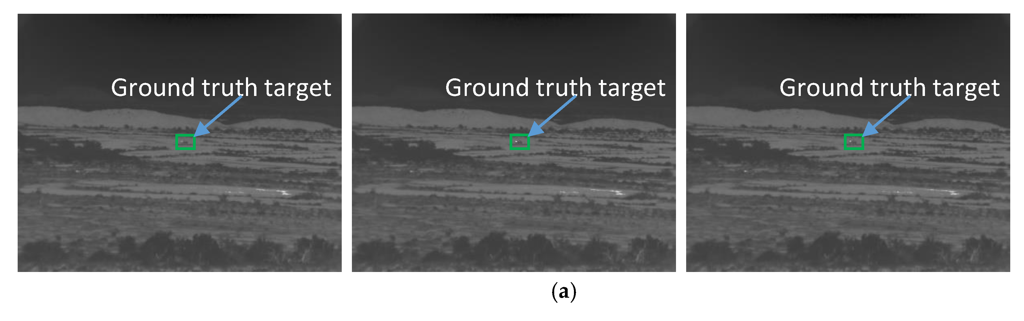
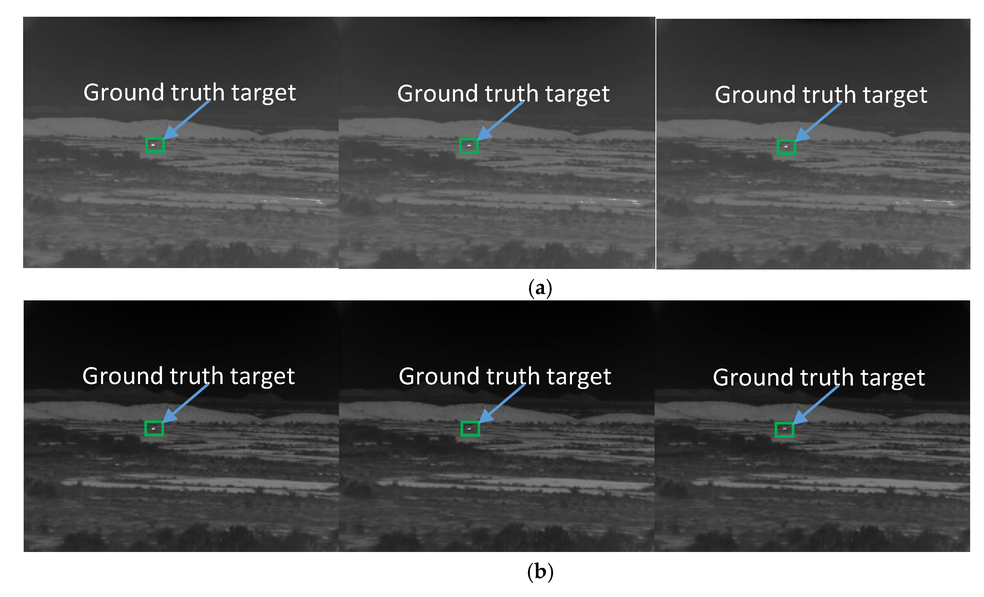
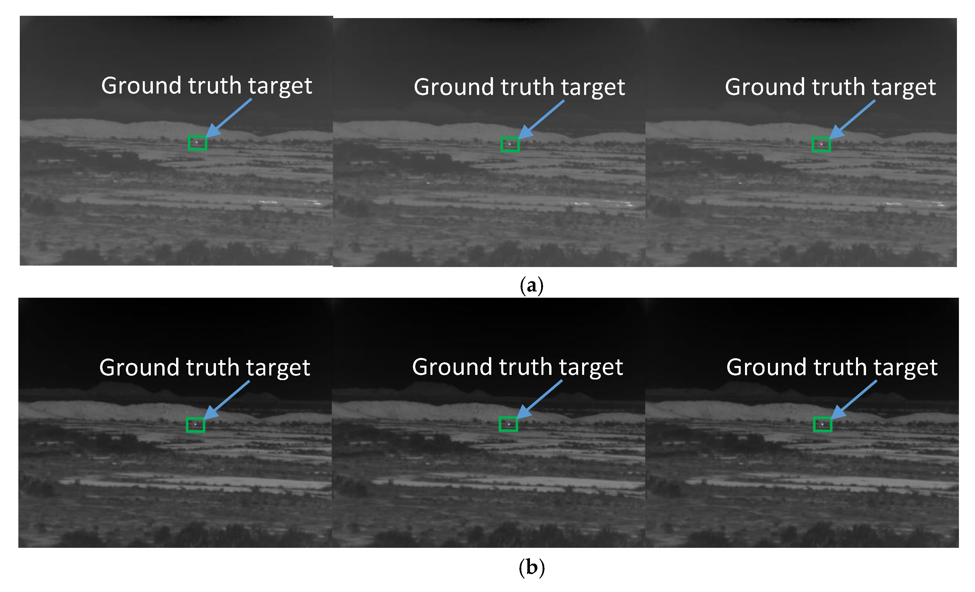
In order to better extract the motion in the frames, the input frame pair is the current frame and the 20th frame from the current frame. This was an important adjustment to the optical flow approach for the DSIAC videos because at the farther distances the motion of the vehicle was relatively minute. By using frames that are farther apart, the motion of the vehicle becomes much more apparent.
Since the image quality is not good, we improved the quality of the input frames within the workflow using contrast enhancement. Different algorithms can yield quite different target detection results. Details can be found in the Appendix A.
Step 2:
Optical flow
The first step is to use TV-L1 or Brox for generating the motion vectors. The basic principles of TV-L1 and Brox were described in Section 2.1.
Step 3:
Intensity mapping
A pair of frames is fed into the TV-L1 or Brox method. The optical flow in the horizontal and vertical (u,v) directions are then transferred to the custom intensity mapping block. Using Algorithm 1 below, we then map the amplitude of the motion vectors into an intensity map. It should be noted that we have incorporated an idea of using the product of intensity and pixel amplitude to weigh the optical flow intensity. This is necessary because, in some dark regions, there are strong motions due to air turbulence. Since the pixel amplitude is quite low in the dark regions, this will mitigate the motion detected in the dark background regions.
Algorithm 1: Weighted optical flow intensity mapping of optical flow image
Input: Horizontal (u) and vertical (v) components of the optical flow and pixel amplitude
P(i,j) of the current frame
Output: Intensity map I
For each pixel location (i,j), compute
(1) |u|, |v|
(2) Normalize |u| and |v| between 0 and 1
(3) Compute weighted optical flow intensity map of I(i,j) = sqrt(u2+v2) * P(i, j)
Step 4:
Segmentation
We used Algorithm 2 below for target segmentation.
Algorithm 2: Target segmentation
Input: Intensity image, I, of the optical flow
Output: Binarized image
(1) Compute the mean of I
(2) Compute standard deviation of I: std(I)
(3) Scan through the image; set pixel to 1 if | | I n e a n ( I ) | | > α *std(I); α should be between 2 and 4; otherwise, set pixel to 0.
Step 5:
Connected component (CC) Analysis to the intensity map
Since the segmented results may have scattered pixels, we then perform connected component analysis on the segmented binarized image to find clusters of moving pixels between frames. Unlike the LIG workflow in [30], there is no use of dilation. Instead, the connected component analyses are using several rules to check whether the connected component is a valid detection or not. These rules involve checking if the area of the connected component is reasonable as well as comparing the max intensity of pixels between the connected components. If the area is over 1 pixel and less than 100 pixels, it is valid. Out of the remaining connected components, the one with the pixel with the highest intensity is then chosen as the target.
Step 6:
Target Association between frames
This workflow has several key differences from the LIG method in [30]. Instead of using information from a single frame to determine the location of a target, one key new component is that we utilize a window of frames to better detect targets. The information of targets from past frames can provide useful information for the potential location of future targets. The current frame and the four previous frames are used to determine the location of a target in the current frame. We then utilize SORT to perform track association of the various detections across these frames. SORT will assign a tracking identity (ID) to each individual frame in the sliding window. The algorithm then selects the ID with the most occurrences within that sliding window as the most likely candidate to be the target. SORT uses target size, target speed, and direction as part of its algorithm to determine track association.
We would like to point out that we also experimented with an alternative target association scheme based on rules. In some cases, the rule-based approach worked better than the SORT algorithm.
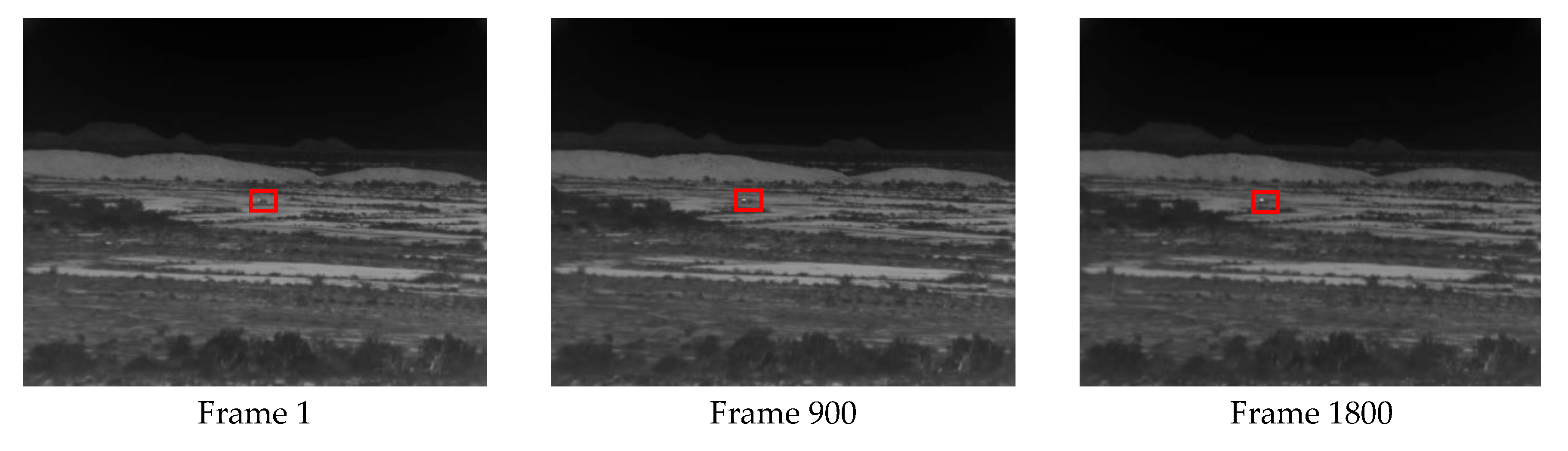
Figure 3 better illustrates how the proposed workflow operates for a given set of frames. However, since there are missing detections in certain frames, it can disrupt the workflow and create negative effects for later frames. In order to resolve this problem, we used a simple extrapolation idea to estimate detections. Extrapolation allows us to estimate the next location of the target by using the previous frames. We take the difference in centroid location of the previous two frames and add this to the previous centroid and use that extrapolated centroid as the location for the target in the current frame. This is now implemented within the SORT module.

2.4. An Alternative Implementation without Using SORT

From the contrast enhancement results in the Appendix A, it was still concerning to see Approach 3a, which is the best contrast enhancement method for all videos, underperforms Approach 1 in the 3500 m case. Upon further investigation, the SORT tracking association method in 
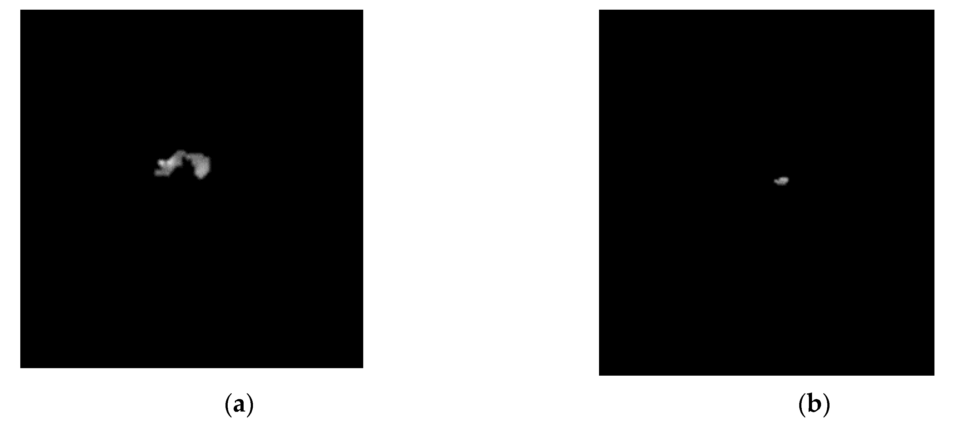
Section 2.3 was not working as intended. SORT pays close attention to the target sizes and when we use optical flow, the target size of the detections can dramatically shift from frame to frame. SORT will assign different tracking IDs to these detected targets because their target sizes are too different for it to associate as the same target. There are two root causes of this issue. First, when performing dilation, nearby connected components can get merged in with the target connected component. Second, the actual size of the detection varies across frames due to natural fluctuation of pixel values. Figure 4 below illustrates the variation of detected target size across frames.
Because of these inherent issues of using SORT, we revisited the original pipeline (Figure 2) and revised it to the flow shown in Figure 5 to see if we could further improve the overall system performance. The majority of the pipeline was left intact, but the rules analysis module shown in Figure 5 was revised. In particular, we updated the sequencing of the rules analysis module. One of the issues with the earlier rules module was that it placed more emphasis on the maximum intensity of a connected component than its location. Our initial assumption was that the target would consistently have the highest optical flow value. Although this assumption is true to a certain extent, there are still a significant amount of cases that did not follow this assumption. Instead, the focus should be on finding relatively high intensity components in a tight range around previous detections.
Details of some rules are summarized in the following sections.

2.4.1. Nearest Neighbor Target Association Using Rules

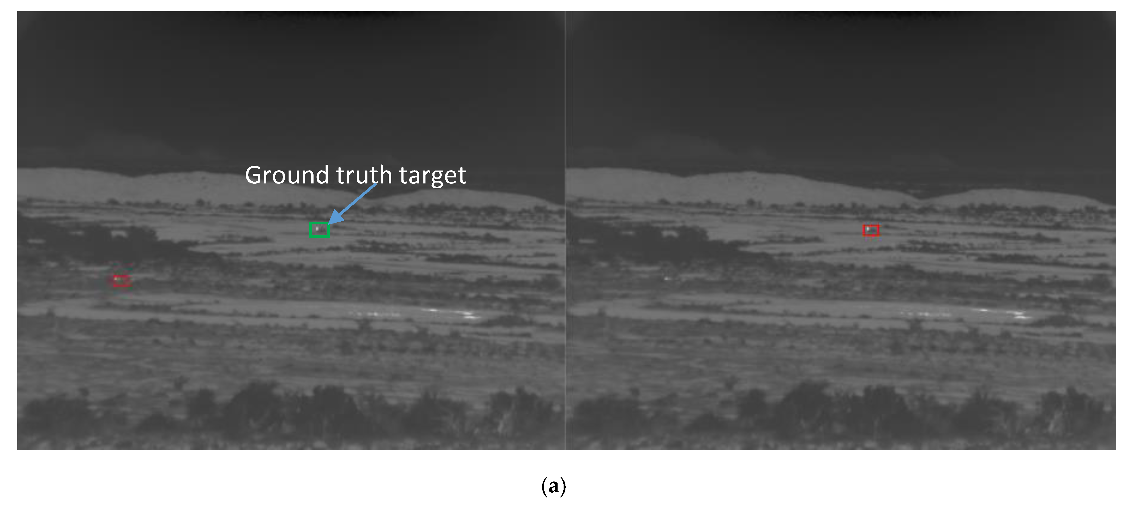
To further reduce false positives, we implemented a simple distance rule to properly associate the components from one frame to another. For example, if we know the location of the target in the previous frame, we can assume that the target did not leave the surrounding area (i.e., 100 pixel radius). When implemented into the optical flow workflow, the results were discouraging. There were 0 correct detections on the 3500 m MWIR daytime video. The reason for this is that if the detected target is far enough outside the actual location of the target, this approach will struggle to correctly detect the target in future frames. The example below demonstrates the shortcomings of this approach for this particular dataset. For example, in the first frame of the 3500 m video, the detected target is in the bottom left. Even though the optical flow correctly detects targets in the proceeding frame, the rule-based analysis will eliminate it from the possible targets due to the original detection in the first frame.

2.4.2. Target Searching Radius

In the updated pipeline shown in Figure 5, there is more emphasis on establishing the initial location of the target and searching closely around that area. We use a much tighter radius for searching, 20 pixels instead of 200. Although there can be cases of missing detections with such a tight search radius, if we use this in conjunction with extrapolation, we can overcome the issue of missing detections. It should be noted that the input frames for this workflow are the Approach 3a contrast-enhanced frames discussed in the Appendix A.

2.4.3. Rules to Eliminate False Positives

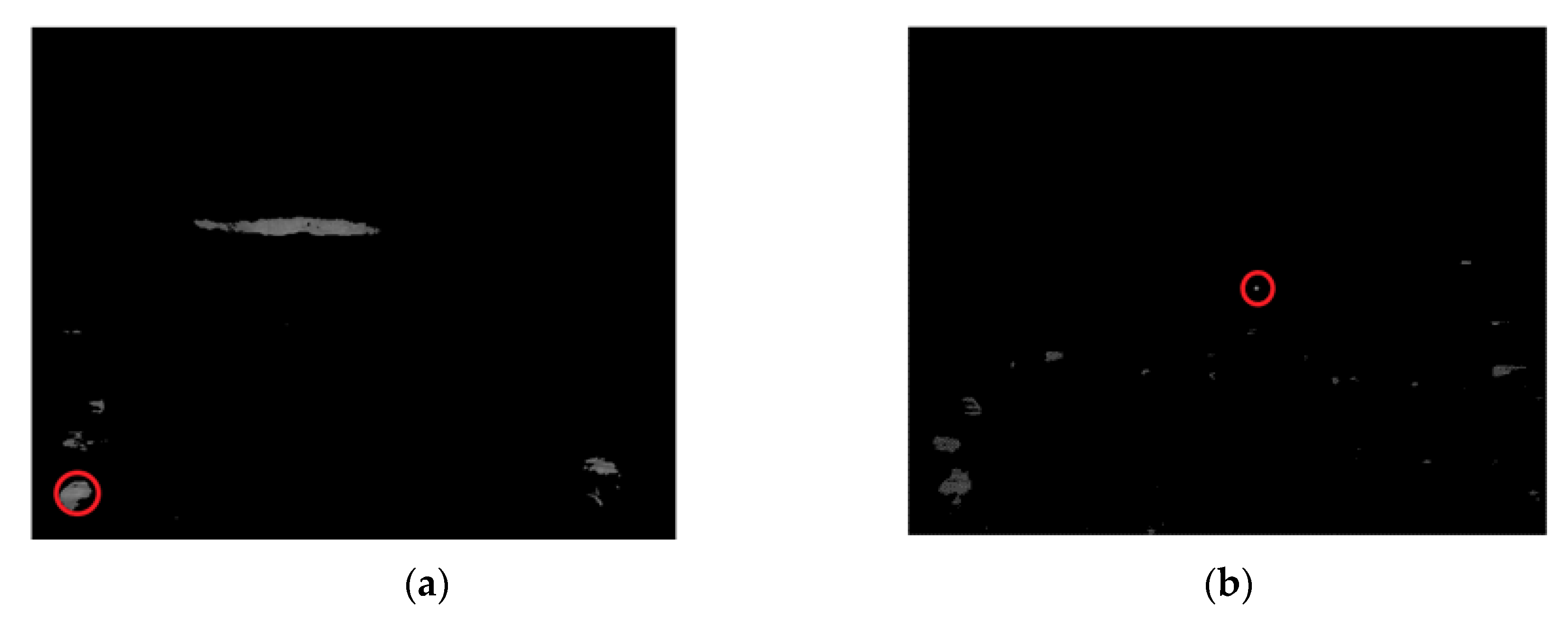
Some simple rules are applied to eliminate some false positives. For example, one rule eliminates certain connected components that do not meet size criteria. If the size of the component is bigger than 10 pixels (for instance), then the component is discarded. 
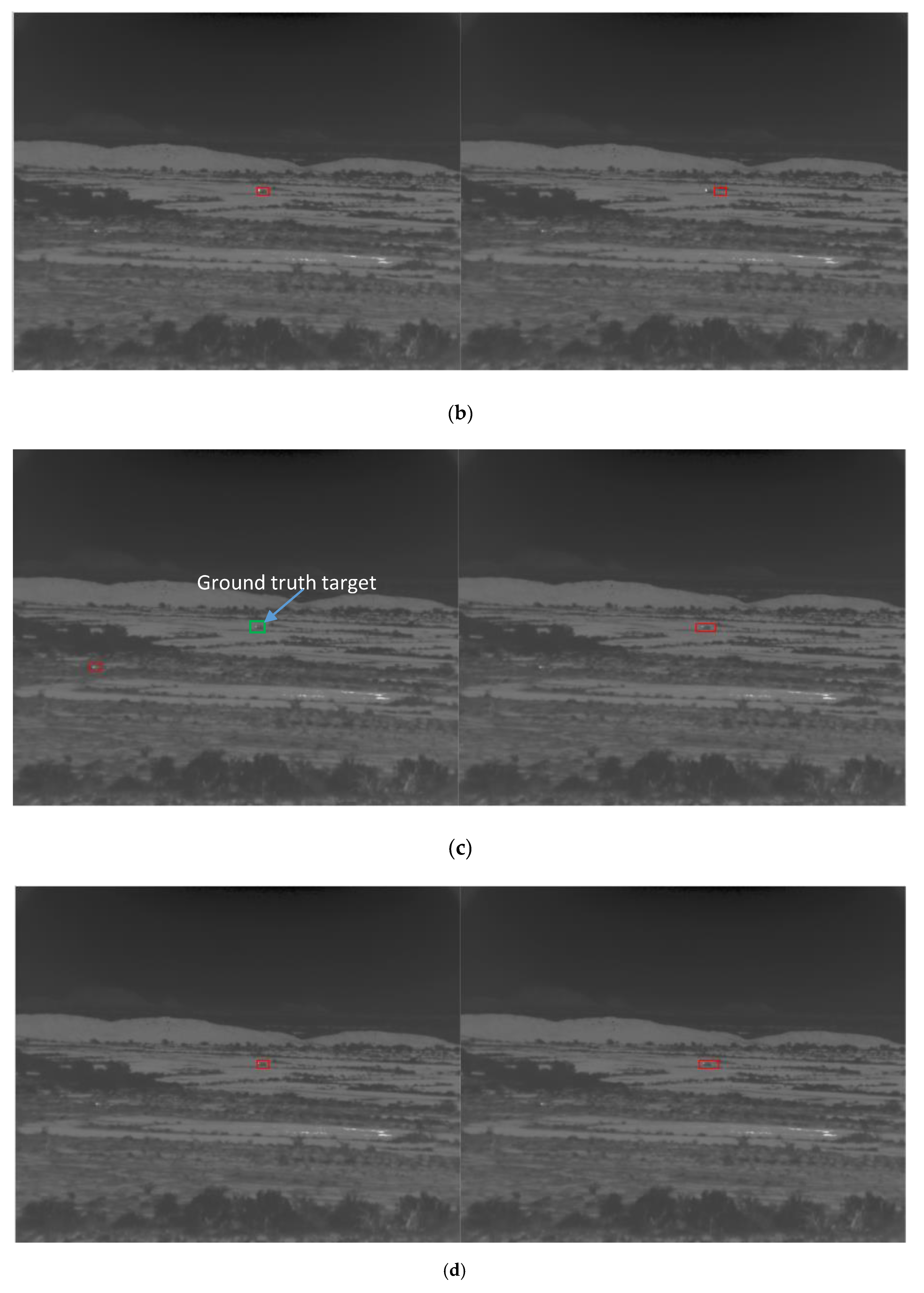
Figure 6 illustrates the impact of using rules. It can be observed that there are more false positives in the image without using rules.

3. Experiments

3.1. Videos

We used four videos in the DSIAC dataset [34]. There are MWIR daytime and night-time videos ranging from 1000 to 5000 m in 500 m increments. We selected four daytime MWIR videos in the following ranges: 3500, 4000, 4500, and 5000 m. Figure 7, Figure 8, Figure 9 and Figure 10 show several frames from each video. It should be noted that contrast enhancement has been applied to these videos. A comparison of five different contrast enhancement approaches was carried out and the results are summarized in the Appendix A. It can be seen that the vehicles (small bright spots inside the red bounding boxes) are hard to see and are quite small in size.

3.2. Performance Metrics

A correct detection or true positive (TP) occurs if the binarized detection is within a certain threshold of the centroid of the ground truth bounding box. Otherwise, the detected object is regarded as a false positive (FP). If a frame does not have TP, then a missed detection (MD) occurs. Based on the correct detection and false positives counts, we can further generate precision, recall, and F1 metrics. The precision (P), recall (R), and F1 are defined as
P =   T P T P + F P
R = T P T P + M D
F 1 =   2 × P × R P + R

3.3. Results Using TV-L1 for Optical Flow in the Proposed Python Workflows

The proposed Python workflows in Section 2.3 and Section 2.4 include a sliding window containing more image pairs, a TV-L1 algorithm, an intensity mapping module, a segmentation module, a CC analysis modules, and a track association algorithm (SORT or rules). As can be seen from Table 1, the results of the workflow with SORT are quite promising except for the 3500 m case. The results in Table 1 show the metrics of the alternative workflow in which the SORT was replaced with some rules. The results are quite impressive as all ranges have an F1 scores higher than 0.9. The 3500 m range has significant improvement over the same 3500 m range in Table 1.
The results in Table 1 show that the alternative approach using rules for target association performed better than SORT. It should be noted that the P, R, and F1 are all the same in those results simply because the numbers of missed detections and false positives are the same.

3.4. Results Using Brox for Optical Flow Generation within Workflows

We conducted a comparative study of the previous two pipelines: SORT-based workflow (Section 2.3) and rule-based workflow (Section 2.4) by utilizing the Brox method as a replacement for TV-L1 [32]. In the past, Brox [33] has shown promising results in a variety of datasets, and we wanted to determine whether it would be effective for an MWIR dataset as well. We ran the two workflows discussed in Section 2.3 and Section 2.4 but with the Brox as the method of choice for calculating optical flow. It is important to note that the frames fed to Brox were contrast enhanced using Approach 3a in the Appendix A. The results across the ranges are presented in Table 2. It should be noted that the P, R, and F1 are all the same in those results simply because the numbers of missed detections and false positives are the same.
The results demonstrate that the SORT-based workflow is effective at all ranges when combined with the Brox method. Previously when using the TV-L1 within this workflow, the 3500 m videos struggled in comparison to the rule-based workflow. This highlights how the two workflows will diverge in effectiveness depending on the method used to calculate optical flow.

3.5. Subjective Evaluations

We have included several frames from the 3500 m video to showcase how the detections differ depending on the method and workflow used. In Figure 11a,c we see some false positives when using the SORT method for target association.

3.6. Comparison of F1 Values Using Different Methods

In Section 1, we mentioned an earlier method [30] developed by us. The idea did not use optical flow to detect objects in each frame. Here, we would like to compare the F1 scores of non-optical flow based approach and optical flow based methods. Table 3 summarizes the comparisons. There are two comparative studies:
  • Comparison of different methods with SORT in the pipelines
    Table 3 summarizes the comparative studies. Within the optical flow category, there are two methods: TV-L1 and Brox. First, it can be seen that the Brox performs more consistently than TV-L1 in all ranges. In particular, TV-L1 did not perform well for the 3500 m video. Second, Brox has comparable performance as the LIG method [30].
  • Comparison of different methods without SORT in the pipelines
    Table 3 summarizes the comparisons between non-optical flow and optical flow-based methods. Rules were used in the object association part. We have three observations. First, TV-L1 is better than Brox this time. Second, the optical flow methods are inferior to the non-optical flow method. Third, based on the results in Table 3, the non-optical flow method is quite consistent in performance in both SORT and rule based cases.

3.7. Computational Times

Although the results are quite impressive for all the optical flow methods, they differ greatly in computational times. Table 4 compares the computational time for the various optical flow methods and an earlier method. These times indicate the time it takes each method to process 300 pairs of frames of size 512 × 640. Table 4 shows the time it takes the individual optical flow methods to process these frames and Table 5 shows the time it takes the remaining modules of the workflow to process those same frames. It can be seen that TV-L1 achieves real-time processing. The TV-L1 method is significantly faster than any other method. Part of the reason for this is its written and optimized in C. In addition, we are using a precompiled executable version of this code. The other methods are not precompiled and are written in MATLAB, a considerably slower language. The TV-L1 at just 0.261 s per frame can be utilized even in real-time applications.
We would like to emphasize that the comparisons in Table 4 may not be fair to Brox’s algorithm and also the method in [30] because those codes were implemented in Matlab. Brox’s algorithm was developed and implemented in Matlab in 2004. We tried to convert those Matlab codes to C by using some Matlab conversion tools. However, this is not a small task. Some commands need to be rewritten. We then abandoned this effort because it is out of the scope of our research.
We would also like to further add a few cautionary notes about the speed between C and Matlab. In one discussion (https://rb.gy/rfnpa6), it was claimed that “Matlab is between 9 to 11 times slower than the best C++ executable.” Another thread from Mathworks (https://rb.gy/nawws1) mentioned that if one optimizes Matlab by pre-allocating memory, using parfor, etc., Matlab codes can also run faster and may be getting very close to the speed of C/C++. Based on our own experience, in some applications, Matlab and C do not differ that much. This is because some Matlab commands such as parfor can utilize multiple cores to speed up processing. In any event, let us suppose that Matlab is indeed 11 times slower than C. Moreover, suppose that we have a C version of Brox, which runs 11 times faster than its Matlab version. This C version still needs roughly 159 s for 300 frames and this is about two times slower than that of TV-L1. For the method in [30], even if we implement the LIG in C, it will still need to take 2000 s per 300 frames, which may still be too slow for real-time applications.
The difference in computational time between workflows in Table 5 is negligible. Both workflows could be used interchangeably in both real-time and offline applications.

4. Conclusions and Future Research

We propose an unsupervised, modular, flexible, and computationally efficient target detection approach for long-range and low-quality infrared videos containing moving objects. Extensive experiments using MWIR infrared videos collected from 3500 to 5000 m were used in our evaluations. Two well-known optical flow methods (TV-L1 and Brox) were used to detect moving objects. Compared with TV-L1, Brox appears to have a slight edge in terms of accuracy, but requires more computational time. Two object association methods were also examined and compared. The rule-based approach outperforms another method known as SORT. We also observed that the manipulation of the intensity/contrast of the input frames is especially essential for optical flow methods, as they are much more sensitive to background intensity differences across frames. Using a second order histogram matching method for contrast enhancement was shown to be effective at resolving contrast issues in the DSIAC dataset.
In the future, we will investigate faster implementation of optical flow methods using C or field programmable gate array (FPGA).

Author Contributions

Conceptualization, C.K.; methodology, C.K.; software, B.B.; validation, C.K. and B.B.; resources, C.K.; data curation, B.B.; writing—original draft preparation, C.K.; writing—review and editing, B.B.; supervision, C.K.; project administration, C.K.; funding acquisition, C.K. All authors have read and agreed to the published version of the manuscript.

Funding

This work was partially supported by US government Payroll Protection Program (PPP) program. The views, opinions and/or findings expressed are those of the author(s) and should not be interpreted as representing the official views or the U.S. Government.

Conflicts of Interest

The authors declare no conflict of interest.

Appendix A

The raw videos are with a bit depth of 16. One frame with 16-bit is shown in Figure A1. It can be seen that the image can be dark sometimes and hence contrast enhancement is needed.
Figure A1. 16-bit raw frame.
Remotesensing 12 04024 g0a1
We experimented with several different approaches to enhance the contrast of these raw frames. We used the following approaches:

Appendix A.1. Approach 1: Histogram Matching to an 8-Bit Reference Frame

In our past study, we have come across an infrared image (8-bit) with good contrast. The first method attempted was simply histogram matching the 16-bit raw image to that 8-bit reference image. The biggest difference in quality was that the image was no longer being saved in a JPEG format and therefore was not losing data each time it was saved, in combination with the increased data quality from using a 16-bit image rather than an 8-bit image.
Approach 1 was implemented using the MATLAB function imhistmatch. The issue with this is that, when a 16-bit image is histogram matched to an 8-bit image, the bit depth of the original image is still 8-bit. In addition, it can be seen from Figure A2 that there are overly bright areas in the background.
Figure A2. Before and after comparison of applying Approach 1. (a) Raw image; (b) Contrast-enhanced image.
Remotesensing 12 04024 g0a2

Appendix A.2. Approach 2: Gamma Correction

Gamma correction is a well-known contrast enhancement technique. We denote the pixel values of an input image that needs contrast enhancement and the enhanced image by x and y, respectively. Gamma correction is expressed as
y = x γ
where γ is a constant. It should be noted that x, y are normalized between 0 and 1. For smaller γ , dark pixels are enhanced; for larger γ , the bright pixels are suppressed.
Approach 2 utilizes the gamma parameter within the imadjust function in MATLAB to enhance the contrast. Gamma correction adjusts the mapping between input pixel amplitudes and output pixel amplitudes. A gamma value of 0.75 was used in our studies. Figure A3 shows the before and after images of gamma correction.
Figure A3. Before and after comparison of Approach 2. (a) Raw image; (b) Contrast-enhanced image.
Remotesensing 12 04024 g0a3

Appendix A.3. Approach 3: Second Order Histogram Matching

Approach 1 used an 8-bit video frame as reference. As a result, the 16-bit low contrast videos are matched to 8-bit intervals. This is undesirable because it will be better to retain the 16-bit data quality in the raw data. Here, we applied a simple second-order contrast enhancement method that has been widely used in remote sensing [37]. This method can preserve the 16-bit data quality in the raw data and is a simple normalization and histogram matching algorithm denoted by
J = r e f s t d I s t d ( I I m e a n ) + r e f m e a n
In the equation, J is the resulting image, refstd is the numeric distance between standard deviations in the reference image, Istd is the numeric distance between standard deviations in the original image, Imean is the mean value of the original image, and refmean is the mean value of the reference image. The reference image used was an image from the middle of the BTR70 vehicle video that is compressed to 8 bits as it has the best histogram of any set of images.
Approach 3 uses a simple formula found in [37] to perform histogram matching. Figure A4 shows one example of the images before and after applying Approach 3.
Figure A4. Before and after comparison of Approach 3. (a) Raw image; (b) Contrast-enhanced image.
Remotesensing 12 04024 g0a4

Appendix A.4. Approach 3a: Intensity Shifting

In some cases, even after the second order histogram matching, the enhanced image still looks dark. For those images, we increase the mean intensity of the whole image by a small amount such as 0.1 to 0.3. Approach 3a is a variation of Approach 3 where we simply add a value to all pixels in order to shift up the mean pixel value of the frame. It is important to utilize a single reference frame for this approach; otherwise, there will be intensity differences across frames. Figure A5 shows the images before and after using Approach 3a.
Figure A5. Before and after comparison of Approach 3a. (a) Raw image; (b) Contrast-enhanced image.
Remotesensing 12 04024 g0a5

Appendix A.5. Approach 4: Reduce Haze

The next method [38] takes the complement of the image, uses a function designed to reduce haze in an image, and then takes the complement of the reduced image. The function reducing haze has an option to also contrast enhance the image. While the contrast enhancement was effective, at times it was too extreme, resulting in the overexposure of specific positions in the image and therefore a loss of data.
Approach 4 uses the imreducehaze function in MATLAB that is commonly used in low-light situations. It will reduce haze and improve contrast based on the inputted estimated haze and estimate lighting conditions. Figure A6 shows one example of the images before and after applying Approach 4.
Figure A6. Before and after comparison of Approach 4. (a) Raw image; (b) Contrast-enhanced image.
Remotesensing 12 04024 g0a6

Appendix A.6. Objective Comparison of the Different Contrast Enhancement Approaches

Although Approach 3 appeared visually superior to other approaches, we need to further validate through objective measures. We compared using these various approaches within the workflow for the 3500 m range. We chose the 3500 m video as this seems to be the most difficult of the ranges. Since we did not record those videos, we can only speculate the potential cause for this abnormal behavior. One possible explanation is that the 3500 m video might be taken on a hot summer day. Because the experimental location was in a desert, the hot air created some turbulence and consequently affected the image quality. Based on our past work [30], the approaches that work well with the 3500 m also translate well to the farther ranges. The performance metrics are shown in Table A1. The performance metrics can vary considerably with different enhancement methods. It can also be seen that Approach 1 has the best overall performance as compared to the other approaches. Moreover, Approach 1 and Approach 3a are better than others. We display a few snapshots of the images after applying Approaches 1 and 3a in Figure A7.
Table A1. Performance metrics for contrast-enhanced approaches within the proposed Python workflow with SORT for 3500 m range. Bold are the best results.
Contrast Enhancement Approaches for 3500 m
PRF1
Approach 10.7870.7900.788
Approach 20.3280.3070.317
Approach 30.6520.6520.652
Approach 3a0.7720.7720.772
Approach 40.8030.5070.622
Figure A7. Three Frames from 3500 m for Approach 1 and 3a. (a) Approach 1; (b) Approach 3a.
Remotesensing 12 04024 g0a7aRemotesensing 12 04024 g0a7b
It was rather unusual to see that the first approach performed better than the other approaches, since this is reducing the bit depth of the frame. However, when we compare Approach 1 and Approach 3a across other ranges in Table A2, Approach 3a, which maintains the bit depth of the raw frame, performs better than Approach 1. Figure A8, Figure A9 and Figure A10 display the enhanced images using Approaches 1 and 3a for videos in the 4000 m, 4500 m, and 5000 m ranges, respectively.
Because of the above experiments, we have decided to use Approach 3a in all of our experiments in our paper.
Table A2. Performance metrics for contrast-enhanced approaches within optical flow workflow for 4000–5000 m ranges. TV-L1 was used for optical flow generation.
(a) Contrast Enhancement Approaches for 4000 m
PRF1
Approach 10.9310.9340.933
Approach 3a0.9660.9660.966
(b) Contrast Enhancement Approaches for 4500 m
PRF1
Approach 10.8630.8660.864
Approach 3a0.9830.9830.983
(c) Contrast Enhancement Approaches for 5000 m
PRF1
Approach 10.9240.9210.922
Approach 3a0.9520.9520.952
Figure A8. Three frames from 4000 m for Approach 1 and 3a. (a) Approach 1; (b) Approach 3a.
Remotesensing 12 04024 g0a8
Figure A9. Three frames from 4500 m for Approach 1 and 3a. (a) Approach 1; (b) Approach 3a.
Remotesensing 12 04024 g0a9
Figure A10. Three frames from 5000 m for Approach 1 and 3a. (a) Approach 1; (b) Approach 3a.
Remotesensing 12 04024 g0a10

References

  1. Kwan, C.; Chou, B.; Kwan, L.M. A Comparative Study of Conventional and Deep Learning Target Tracking Algorithms for Low Quality Videos. In Proceedings of the 15th International Symposium on Neural Networks, Minsk, Belarus, 25–28 June 2018. [Google Scholar]
  2. Demir, H.S.; Cetin, A.E. Co-difference based object tracking algorithm for infrared videos. In Proceedings of the IEEE International Conference on Image Processing (ICIP), Phoenix, AZ, USA, 25–28 September 2016; pp. 434–438. [Google Scholar]
  3. Kwan, C.; Chou, B.; Yang, J.; Tran, T. Compressive object tracking and classification using deep learning for infrared videos. In Proceedings of the Pattern Recognition and Tracking (Conference SI120), Baltimore, MD, USA, 13 May 2019. [Google Scholar]
  4. Kwan, C.; Chou, B.; Yang, J.; Tran, T. Target tracking and classification directly in compressive measurement for low quality videos. In Proceedings of the SPIE 10995, Pattern Recognition and Tracking XXX, Baltimore, MD, USA, 13 May 2019; Volume 1099505. [Google Scholar]
  5. Kwan, C.; Chou, B.; Echavarren, A.; Budavari, B.; Li, J.; Tran, T. Compressive vehicle tracking using deep learning. In Proceedings of the IEEE Ubiquitous Computing, Electronics & Mobile Communication Conference, New York, NY, USA, 8–10 November 2018. [Google Scholar]
  6. Kwan, C.; Gribben, D.; Tran, T. Multiple Human Objects Tracking and Classification Directly in Compressive Measurement Domain for Long Range Infrared Videos. In Proceedings of the IEEE Ubiquitous Computing, Electronics & Mobile Communication Conference, New York, NY, USA, 10–12 October 2019. [Google Scholar]
  7. Kwan, C.; Gribben, D.; Tran, T. Tracking and Classification of Multiple Human Objects Directly in Compressive Measurement Domain for Low Quality Optical Videos. In Proceedings of the IEEE Ubiquitous Computing, Electronics & Mobile Communication Conference, New York, NY, USA, 10–12 October 2019. [Google Scholar]
  8. Kwan, C.; Chou, B.; Yang, J.; Tran, T. Deep Learning based Target Tracking and Classification Directly in Compressive Measurement for Low Quality Videos. Signal Image Process. 2019, 10, 6. [Google Scholar] [CrossRef]
  9. Kwan, C.; Chou, B.; Yang, J.; Rangamani, A.; Tran, T.; Zhang, J.; Etienne-Cummings, R. Target tracking and classification directly using compressive sensing camera for SWIR videos. J. Signal Image Video Process. 2019, 13, 1629–1637. [Google Scholar] [CrossRef]
  10. Kwan, C.; Chou, B.; Yang, J.; Rangamani, A.; Tran, T.; Zhang, J.; Etienne-Cummings, R. Target tracking and classification using compressive measurements of MWIR and LWIR coded aperture cameras. J. Signal Inf. Process. 2019, 10, 73–95. [Google Scholar] [CrossRef] [Green Version]
  11. Kwan, C.; Gribben, D.; Rangamani, A.; Tran, T.; Zhang, J.; Etienne-Cummings, R. Detection and Confirmation of Multiple Human Targets Using Pixel-Wise Code Aperture Measurements. J. Imaging 2020, 6, 40. [Google Scholar] [CrossRef]
  12. Kwan, C.; Chou, B.; Yang, J.; Tran, T. Deep Learning based Target Tracking and Classification for Infrared Videos Using Compressive Measurements. J. Signal Inf. Process. 2019, 10, 167. [Google Scholar] [CrossRef] [Green Version]
  13. Kwan, C.; Chou, B.; Yang, J.; Rangamani, A.; Tran, T.; Zhang, J.; Etienne-Cummings, R. Deep Learning based Target Tracking and Classification for Low Quality Videos Using Coded Aperture Camera. Sensors 2019, 19, 3702. [Google Scholar] [CrossRef] [Green Version]
  14. Lohit, S.; Kulkarni, K.; Turaga, P.K. Direct inference on compressive measurements using convolutional neural networks. Int. Conf. Image Process. 2016, 1913–1917. [Google Scholar]
  15. Adler, A.; Elad, M.; Zibulevsky, M. Compressed Learning: A Deep Neural Network Approach. arXiv 2016, arXiv:1610.09615v1. [Google Scholar]
  16. Xu, Y.; Kelly, K.F. Compressed domain image classification using a multi-rate neural network. arXiv 2019, arXiv:1901.09983. [Google Scholar]
  17. Wang, Z.W.; Vineet, V.; Pittaluga, F.; Sinha, S.N.; Cossairt, O.; Kang, S.B. Privacy-Preserving Action Recognition Using Coded Aperture Videos. In Proceedings of the IEEE Conference on Computer Vision and Pattern Recognition (CVPR) Workshops, Long Beach, CA, USA, 16–20 June 2019. [Google Scholar]
  18. Vargas, H.; Fonseca, Y.; Arguello, H. Object Detection on Compressive Measurements using Correlation Filters and Sparse Representation. In Proceedings of the 26th European Signal Processing Conference (EUSIPCO), Roma, Italy, 3–7 September 2018; pp. 1960–1964. [Google Scholar]
  19. Değerli, A.; Aslan, S.; Yamac, M.; Sankur, B.; Gabbouj, M. Compressively Sensed Image Recognition. In Proceedings of the 7th European Workshop on Visual Information Processing (EUVIP), Tampere, Finland, 26–28 November 2018. [Google Scholar]
  20. Latorre-Carmona, P.; Traver, V.J.; Sánchez, J.S.; Tajahuerce, E. Online reconstruction-free single-pixel image classification. Image Vis. Comput. 2018, 86, 28–37. [Google Scholar] [CrossRef]
  21. Kwan, C.; Gribben, D.; Chou, B.; Budavari, B.; Larkin, J.; Rangamani, A.; Tran, T.; Zhang, J.; Etienne-Cummings, R. Real-Time and Deep Learning based Vehicle Detection and Classification using Pixel-Wise Code Exposure Measurements. Electronics 2020, 9, 1014. [Google Scholar] [CrossRef]
  22. Li, C.; Wang, W. Detection and Tracking of Moving Targets for Thermal Infrared Video Sequences. Sensors 2018, 18, 3944. [Google Scholar] [CrossRef] [PubMed] [Green Version]
  23. Tan, Y.; Guo, Y.; Gao, C. Background subtraction based level sets for human segmentation in thermal infrared surveillance systems. Infrared Phys. Technol. 2013, 61, 230–240. [Google Scholar] [CrossRef]
  24. Berg, A.; Ahlberg, J.; Felsberg, M. Channel Coded Distribution Field Tracking for Thermal Infrared Imagery. In Proceedings of the IEEE Conference on Computer Vision and Pattern Recognition Workshops, Las Vegas, NV, USA, 26 June–1 July 2016; pp. 1248–1256. [Google Scholar]
  25. Chen, C.L.P.; Li, H.; Wei, Y.; Xia, T.; Tang, Y.Y. A local contrast method for small infrared target detection. IEEE Trans. Geosci. Remote Sens. 2014, 52, 574–581. [Google Scholar] [CrossRef]
  26. Wei, Y.; You, X.; Li, H. Multiscale patch-based contrast measure for small infrared target detection. Pattern Recognit. 2016, 58, 216–226. [Google Scholar] [CrossRef]
  27. Gao, C.; Meng, D.; Yang, Y.; Wang, Y.; Zhou, X.; Hauptmann, A.G. Infrared patch-image model for small target detection in a single image. IEEE Trans. Image Process. 2013, 22, 4996–5009. [Google Scholar] [CrossRef] [PubMed]
  28. Zhang, L.; Peng, L.; Zhang, T.; Cao, S.; Peng, Z. Infrared small target detection via non-convex rank approximation minimization joint l2,1 norm. Remote Sens. 2018, 10, 1–26. [Google Scholar] [CrossRef]
  29. Zhang, H.; Zhang, L.; Yuan, D.; Chen, H. Infrared small target detection based on local intensity and gradient properties. Infrared Phys. Technol. 2018, 89, 88–96. [Google Scholar] [CrossRef]
  30. Kwan, C.; Budavari, B. A High Performance Approach to Detecting Small Targets in Long Range Low Quality Infrared Videos. arXiv 2020, arXiv:2012.02579. [Google Scholar]
  31. Lucas, B.D.; Kanade, T. An iterative image registration technique with an application to stereo vision. Proc. Imaging Underst. Workshop 1981, 2, 121–130. [Google Scholar]
  32. Zach, C.; Pock, T.; Bischof, H. A Duality Based Approach for Real-Time TV-L1 Optical Flow, Joint Pattern Recognition Symposium; Springer: Berlin/Heidelberg, Germany, 2007; pp. 214–223. [Google Scholar]
  33. Brox, T.; Bruhn, A.; Papenberg, N.; Weickert, J. High accuracy optical flow estimation based on a theory for warping. In European Conference on Computer Vision; Springer: Berlin/Heidelberg, Germany, 2004; pp. 25–36. [Google Scholar]
  34. DSIAC Dataset. Available online: https://www.news.gatech.edu/2006/03/06/sensiac-center-helps-advance-military-sensing (accessed on 8 December 2020).
  35. Available online: https://github.com/vinthony/Dual_TVL1_Optical_Flow (accessed on 8 December 2020).
  36. Bewley, A.; Ge, Z.; Ott, L.; Ramos, F.; Upcroft, B. Simple Online and Realtime Tracking. arXiv 2016, arXiv:1602.00763. [Google Scholar]
  37. Kwan, C.; Kwan, L.; Hagen, L.; Chou, B.; Perez, D.; Li, J.; Shen, Y.; Koperski, K. Simple and effective cloud-and shadow-detection algorithms for Landsat and Worldview images. Signal Image Video Process. 2020, 14, 125–133. [Google Scholar] [CrossRef]
  38. Imreducehaze. Available online: https://www.mathworks.com/help/images/low-light-image-enhancement.html (accessed on 3 December 2020).
Figure 1. Lucas–Kanade (LK) optical flow between Frame 1 and 10 for 3500 m (daytime video).
Remotesensing 12 04024 g001
Figure 2. Proposed optical flow based target detection and tracking workflow. The workflow was implemented in Python.
Remotesensing 12 04024 g002
Figure 3. Example of how the proposed workflow generates detections. The color coding after Simple Online and Real-time Tracking (SORT) is used as a visual representation of the different tracking identities (IDs) assigned to each detection.
Remotesensing 12 04024 g003
Figure 4. Comparison of intensity mapping of target in two sequential frames. (a) Frame 10; (b) Frame 11.
Remotesensing 12 04024 g004
Figure 5. Alternative Python pipeline using rules for target association.
Remotesensing 12 04024 g005
Figure 6. Results using nearest neighbors to associate targets in different frames. (a) Without using rules; (b) With rules.
Remotesensing 12 04024 g006
Figure 7. Frames from the 3500 m video.
Remotesensing 12 04024 g007
Figure 8. Frames from the 4000 m video.
Remotesensing 12 04024 g008
Figure 9. 4500 m daytime videos.
Remotesensing 12 04024 g009
Figure 10. Frames from the 5000 m video.
Remotesensing 12 04024 g010
Figure 11. Comparison of four approaches across 2 different frames in a 3500 m video. (a) Total Variation with L1 constraint (TV-L1) in proposed Python Workflow with SORT (left) and TV-L1 in Alternative Workflow with rules (right); (b) Brox in proposed Python Workflow with SORT (left) and Brox in Alternative Workflow with Rules (right); (c) TV-L1 in proposed Python Workflow with SORT (left) and TV-L1 in Alternative Workflow with Rules (right); (d) Brox in proposed Python Workflow with SORT (left) and Brox in Alternative Workflow with Rules (right).
Remotesensing 12 04024 g011aRemotesensing 12 04024 g011b
Table 1. Results using the proposed workflow for long-range videos.
(a) TV-L1 in Proposed Python Workflow with SORT(b) TV-L1 in Alternative Workflow with Rules
RangePRF1PRF1
3500 m0.7720.7720.7720.9100.9100.910
4000 m0.9660.9660.9660.9900.9900.990
4500 m0.9830.9830.9831.0001.0001.000
5000 m0.9520.9520.9520.9970.9970.997
Table 2. Adjusted rules vs. improved python workflow using Brox optical flow in the pipeline.
(a) Brox in Proposed Python Workflow with SORT(b) Brox in Alternative Workflow with Rules
RangePRF1PRF1
3500 m0.9690.9690.9690.8170.8170.817
4000 m0.9280.9280.9280.8790.8790.879
4500 m0.9690.9690.9690.9660.9660.966
5000 m0.9860.9860.9860.9170.9170.917
Table 3. Comparison of F1 values using different methods. (a) Comparison of F1 values using methods with and without optical flow. SORT was used for object association. Bold numbers indicate the best performing methods; (b) Comparison of F1 values using methods with and without optical flow. Rules were used for object association between frames. Bold numbers indicate the best performing methods.
(a)
Non-Optical Flow (SORT) [30]Proposed Optical Flow Based Workflow (SORT)
Range TV-L1Brox
3500 m0.9740.7720.969
4000 m0.9710.9660.928
4500 m0.9660.9830.969
5000 m0.9770.9520.986
(b)
Non-Optical Flow (Rules) [30]Alternative Optical Flow Based Workflow Using Rules
Range TV-L1Brox
3500 m0.9450.9100.817
4000 m0.9430.9900.879
4500 m0.9551.0000.966
5000 m0.9360.9970.917
Table 4. Comparison of computational times for optical flow methods and an earlier method [30]. Bold numbers indicate the best performing methods.
Optical Flow MethodLanguageTime for 300 Frames (s)
Non-optical flow [30]MATLAB63,000
Non-optical flow Parallel [30] MATLAB22,000
TV-L1C76
BroxMATLAB1750
Table 5. Computational time for workflows excluding optical flow. Bold numbers indicate the best performing methods.
Workflow Excluding Optical FlowTime for 300 Frames (s)
Proposed python workflow with SORT (Section 2.3)14
Alternative workflow with rules (Section 2.4)25
Publisher’s Note: MDPI stays neutral with regard to jurisdictional claims in published maps and institutional affiliations.

