Article

Modelling of River Flow Using Particle Swarm Optimized Cascade-Forward Neural Networks: A Case Study of Kelantan River in Malaysia

by
Gasim Hayder
1,2,*,
Mahmud Iwan Solihin
3 and
Hauwa Mohammed Mustafa
4,5,*
1
Institute of Energy Infrastructure (IEI), Universiti Tenaga Nasional (UNITEN), Kajang 43000, Selangor, Malaysia
2
Department of Civil Engineering, College of Engineering, Universiti Tenaga Nasional (UNITEN), Kajang 43000, Selangor, Malaysia
3
Faculty of Engineering, Technology and Built Environment, UCSI University, Kuala Lumpur 56000, Malaysia
4
College of Graduate Studies, Universiti Tenaga Nasional (UNITEN), Kajang 43000, Selangor, Malaysia
5
Department of Chemistry, Kaduna State University (KASU), Tafawa Balewa Way, Kaduna P.M.B. 2339, Nigeria
*
Authors to whom correspondence should be addressed.
Appl. Sci. 2020, 10(23), 8670; https://doi.org/10.3390/app10238670
Submission received: 5 November 2020 / Revised: 26 November 2020 / Accepted: 26 November 2020 / Published: 4 December 2020

Abstract

:
Water resources management in Malaysia has become a crucial issue of concern due to its role in the economic and social development of the country. Kelantan river (Sungai Kelantan) basin is one of the essential catchments as it has a history of flood events. Numerous studies have been conducted in river basin modelling for the prediction of flow and mitigation of flooding events as well as water resource management. This paper presents river flow modelling based on meteorological and weather data in the Sungai Kelantan region using a cascade-forward neural network trained with particle swarm optimization algorithm (CFNNPSO). The result is compared with those trained with the Levenberg–Marquardt (LM) and Bayesian Regularization (BR) algorithm. The outcome of this study indicates that there is a strong correlation between river flow and some meteorological and weather variables (weighted rainfall, average evaporation and temperatures). The correlation scores (R) obtained between the target variable (river flow) and the predictor variables were 0.739, −0.544, and −0.662 for weighted rainfall, evaporation, and temperature, respectively. Additionally, the developed nonlinear multivariable regression model using CFNNPSO produced acceptable prediction accuracy during model testing with the regression coefficient (R2), root mean square error (RMSE), and mean of percentage error (MPE) of 0.88, 191.1 cms and 0.09%, respectively. The reliable result and predictive performance of the model is useful for decision makers during water resource planning and river management. The constructed modelling procedure can be adopted for future applications.

1. Introduction

Malaysia is enriched with 189 river basins nationwide. This natural resource performs a crucial role in the economic and social development of the country [1]. More specifically, rivers are the major source of water for irrigation, residential, industrial, agricultural, and other human activities. Surface water in the form of streams and rivers contributes 97% of raw water supply [2]. Consequently, due to the over-dependence on surface water for food, recreation, water supply, transportation, and energy, the quality of river water is threatened by various factors [3]. Physicochemical and biological indicators have been used to assess and estimate the quality of river water [4].
Another important aspect of hydrology in Malaysia is water resource management. Water resource management can be defined as a procedure for evaluating the scope, source, quality, and amount of water resources for adequate water resource management and utilization. In the aspect of quantity, artificial neural networks (ANNs) have been employed in previous studies for the prediction of river flow modelling in Malaysia and other countries [5]. For instance, in the case of Malaysian rivers, Mustafa et al. [6] applied a radial basis function (RBF) neural network in forecasting the suspended sediment (SS) discharge of the Pari River. The outcome of the study showed that the RBF neural network models are adequate and they can forecast the nonlinear activity of the suspended solid discharge. Tengeleng and Armand [7] applied cascade-forward backpropagation neural networks to predict rain rate, radar reflectivity and water content with raindrop size distribution. The research was conducted in five localities of African countries; Côte d’Ivoire, Cameroon, Senegal, Congo-Brazaville and Niger.
Furthermore, the performance of two ANNs such as RBF and feed-forward neural networks (FFNN) has been compared in the study of Rantau Panjang streamflow station, Sungai Johor [8]. The result indicated that the FFNN model gave a better performance in estimating the sediment load compared to the RBF model. Memarian and Balasundram [9] compared two other ANNs, namely, Multi-Layer Perceptron (MLP) and RBF for predicting sediment load at Langat River. However, MLP showed better performance, although both ANNs models have demonstrated limited effectiveness in estimating large sediment loads. Similarly, Uca et al. [10] compared the performance of Multiple Linear Regression (MLRg) and ANN in the prediction of SS discharge of the Jenderam catchment area. The ANN methods used are RBF and feed-forward multi-layer perceptron with three learning algorithms, i.e., Broyden–Fletcher–Goldfarb–Shanno Quasi-Newton (BFGS), Levenberg–Marquardt (LM), and Scaled Conjugate Descent (SCD). The effect of different numbers of neurons in the ANN trained with difference algorithms were studied. Moreover, Hayder et al. [1] applied ANN in predicting the physicochemical parameters of Kelantan River. The ANN model was trained by using the optimized value of look back and epoch number. The performance criteria were obtained by calculating the Pearson correlation coefficient (PCC), root mean square error (RMSE), and mean absolute percentage error (MAPE). The findings of the study indicated that the estimation of the pH parameter gave the best performance. Moreover, the lowest kurtosis values of pH suggest that the presence of outliers impacted on the model.
However, artificial neural networks (ANNs) require further elaboration for their experimentations and applications. Machine learning tools, including ANNs, need to be trained before being deployed into real applications to solve a given task. This process is performed in order to identify the best combination of bias and weight values of each neuron by optimizing a cost function that quantifies the mean differences between the predicted and actual output [11]. In light of the above discussion, ANN training is commonly performed using a gradient-based algorithm known as backpropagation (BP) and its variants [12]. Despite its widespread applications in ANN training, the performance of BP algorithm is highly dependent on the weight and bias values of each neuron initialized in the multi-layer ANNs. Furthermore, BP also tends to produce suboptimal solutions of neuron weight and bias values during the training process, hence restricting the performance of ANN [11,12,13]. Recently, there are growing interests in exploiting the excellent global search ability and stochastics natures of metaheuristic search algorithms (MSAs), including Particle Swarm Optimization (PSO) used in this study, to perform ANNs training [11,12,13,14,15,16,17]. As compared to the BP algorithm, MSAs have more competitive advantages in solving ANNs training problems with faster convergence without requiring good initial solutions [11,13].
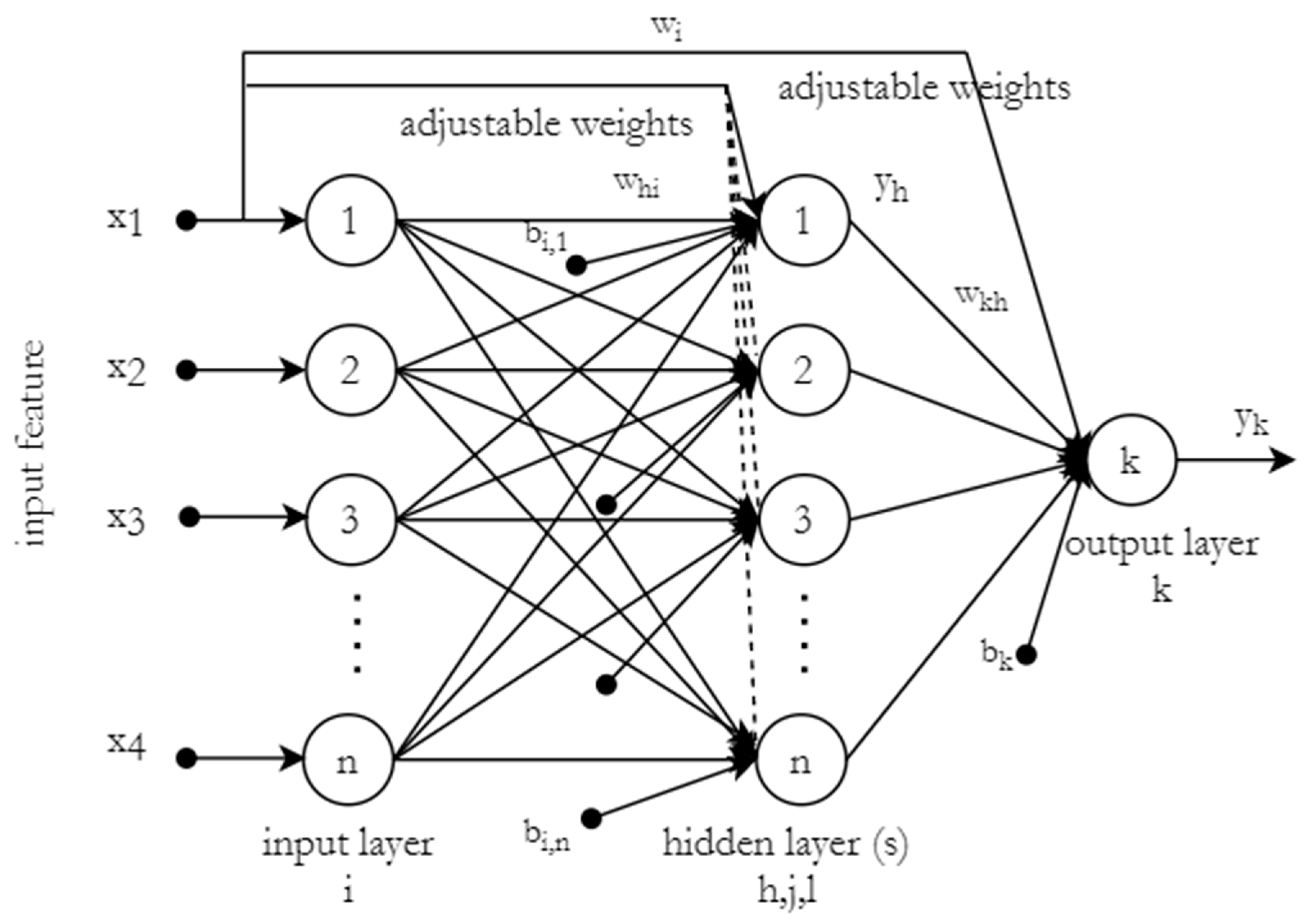
Therefore, this study presents the application of ANNs-based predictive modelling trained using PSO. Particularly, cascade-forward neural networks trained with PSO (CFNNPSO) for the prediction of river flow are presented. This study validates the functional ability and significance of ANN techniques in the simulation of real-world and complex nonlinear water system processes. In addition, this research gives an insight into ANNs modelling in the Kelantan river scenario and the importance of understanding a river basin and variables before attempting to model the river flow. River flow can be effectively modelled with intelligent ANNs models, despite the spatial changes in the study field.
The river flow of Sungai Kelantan in the northeast part of Malaysia is predicted by using FFNN and CFNN based on available meteorological input variables (features) namely; weighted rainfall (mm), evaporation (mm), min of temperature (°C), mean of temperature (°C) and max of temperature (°C). Some of the ANNs-related experimentation carried out in this study includes; feature/input variables selection, the effective number of hidden layer neurons, and performance comparison between CFNN and standard multi-layer FFNN trained with PSO and other common training algorithms such as Levenberg–Marquardt (LM), Bayesian Regularization (BR) backpropagation. This study has practical meaning from the perspective of the current state-of-the-art in artificial intelligence (AI) and the Internet of Things (IoT) technology. The machine learning model can be deployed in different ways, such as using a web app or real-time monitoring device to predict Kelantan river flow based on the readily available meteorological data. The applicability of this tool will be of importance nowadays in the realm of Industrial Revolution 4.0.

2. Materials and Methods

2.1. Study Area

The Kelantan river basin is one of the important catchments as it has a history of flood events [18,19]. The catchment is representing most of the land area of Kelantan State, as shown in Figure 1. There are several stations such as rainfall, water level, evaporation, water quality and meteorological stations operating in the area.

2.2. River Flow Data

ANN is a popular machine learning algorithm that has been successfully applied for data-driven predictive modelling. Therefore, the main ingredient for the success of predictive modelling is the data itself in addition to the training algorithm developed. In this study, the river flow data were used together with meteorological parameters. The river flow data were collected from the north of Kuala Krai city downstream (merge of two main tributaries and before discharge into the sea). Similarly, the original data obtained consist of 348 monthly records of Sungai Kelantan river flow (cubic meters per second (cms)) spanning from January 1988 to December 2016. Rainfall and evaporation are usually measured in a determined station, and only the computed area weighted rainfall is used to evaluate the whole area rainfall quantity [20]. The river flow was mainly from one main station (Guillemard), while the weighted rainfall and evaporation (secondary data) were over the whole river catchment. Table 1 shows the attributes of the data used in this study.

2.3. Data Pre-Processing

The stage of data pre-processing and feature selection process is crucial in the initial stage of the machine learning model building. This process can significantly affect the prediction accuracy in any type of data [21]. The overall data pre-processing and feature selection are summarized as follows:
Data randomization: the data were randomized to enhance the diversity of the data before splitting into training and testing datasets.
Data partition/splitting: datasets were randomly partitioned into training and testing datasets consisting of 260 data samples (≈75%) for model training and 88 data samples (≈25%) for model validation test.
Data normalization: ANNs benefit from data normalization as do some other machine learning algorithms. The input data are normalized to standardize the scale of each variable. In this study, the data are normalized to the range [0,1] before the ANNs training.
Feature selection: feature removal for considerably low correlation score to the output variable. Normally, if the correlation score is less than |0.5|, these variables indicate a low correlation, i.e., a weak association between the specific input variable with the target variable. This process is the most important for predicting the accuracy of this study. It is also useful for model parsimony, especially when the input features are large. The reduced number of input features will give benefit for model simplicity and data reduction in the absence of data collection/sensor measurement. However, the experimentation results of this process are discussed in Section 3. The correlation coefficient ( r x y ) between two variables was calculated by dividing the covariance with the product of the standard deviations of the two variables as follows:
r x y = C o v ( x , y ) σ x σ y

2.4. ANN Structure, Training Algorithm, and Feature Input Selection

ANN is a supervised machine learning that can be trained to map the relation between input/feature and the target/output by adjusting the weights and biases between neuron elements [22]. This highly nonlinear mapping can be applied in many areas, including multivariable regression. There are different types of ANNs structure and training algorithms. Among the common types are cascade-forward neural networks (CFNN), multi-layer feed-forward neural networks (FFNN) and recurrent neural networks. In this study, both FFNN and CFNN structures were implemented, and their effectiveness was compared and evaluated. The programming execution was performed in MATLAB 2019b software. The structure CFNN is similar to FFNN, but the key difference between the two is that CFNN include a connection from the input to the neurons in the following hidden layers. The advantage of this approach is that it accommodates the nonlinear input-output relationship without eliminating the linear relationship between the two [23]. FFNN is a standard structure for a multi-layer neural network which can be found in many works of literature. Additionally, CFNN is a further modification of FFNN where additional weights are connected from the input nodes to the hidden nodes, and output nodes, as shown in the upper portion of Figure 2. These additional weights do not exist in the standard FFNN. The different networks structure between CFNN and FFNN in terms of weight connection can also be seen in the study [7,24]. Detailed computation works about the application of the training algorithms can be found in [7,25].
The output of the CFNN was expressed as:
y ^ k ( x , w ) = i φ ( w i x i ) + φ ( h w k h φ ( j w h j φ ( φ ( i w l i x i + b i ) ) + b j ) + b h )
where φ ( · ) is the selected activation function, w k h is the weight strength from a neuron in the last hidden layer h to the single output neuron k , and so on, for other weights’ strength. x i is the i th element of the input/features variable and b i is the bias weight in the neurons of the first hidden layer, and so on. The symbol w denotes the weight vector for the entire set of all weights ordered by layer, followed by neurons in a layer and then signal strength in a neuron. Hence, in this study, 1 or 2 hidden layers of ANN were used for the evaluation. The activation function selected for the hidden layer(s) and the output layer is the tangent sigmoid and linear function, respectively. The tangent sigmoid function can be expressed as:
φ ( I i ) = 2 1 + e 2 I i 1
where I i is the signal coming into the neuron in hidden layers.
For the linear function in the output layer, it can be expressed as follows:
φ ( I k ) = I k
where I k is the input to the neurons in the output layer.
Furthermore, ANN is usually trained using the backpropagation (BP) algorithm and its variations. Among the commonly used ANN training algorithms is Levenberg–Marquardt (LM), which can provide fast convergence for the moderate-sized FFNN of a few hundredweights [26]. However, fast convergence does not guarantee that the trained ANN model will not overfit the training data. In many applications, including this study, the generalization of the model to the given data is more of concern, i.e., the model will not be either overfitting or underfitting. A more advanced modification of the LM algorithm is called Bayesian Regularization (BR), which reduces the linear combination of squared errors and weights. At the end of the training, the resulting network will have good generalization qualities, i.e., to prevent model overfitting. Further detailed discussions on Bayesian regularization can be seen in [27]. Therefore, for the reason of generalization capability, this algorithm is also applied in this study. Lastly, the PSO algorithm is also applied to train both FFNN and CFNN as the main contribution of this study. The performance of both FFNN and CFNN trained with PSO will be evaluated. PSO is considered the most popular meta-heuristic algorithm inspired by the nature process of bird flocking introduced in 1995 by Kennedy and Eberhart [28,29,30]. It has some appealing features, such as fast convergence speed and simplicity of implementation. Since then many PSOs and their variants have been studied. One of the early PSO variants introduced was PSO with constriction coefficients which was proposed to guarantee solution convergence [30]. This version of PSO will be applied in this study to train the proposed ANN model.
Prior to the discussion of the PSO algorithm used to train ANNs, the basic ANNs training/learning process using the BP algorithm can be summarized as follows [31]:
  • Obtain the training dataset ( x i ) with the desired target ( y ).
  • Setup ANN structure and parameters: number of hidden layers, number of neurons, learning rate ( η ) , momentum constant and regularization constant ( α ) (if necessary).
  • Initialize of all weights and biases to random.
  • Start the ANN training and forward propagation of input data through the layers according to Equation (2).
  • Calculate the error difference between ANN output ( y ^ ) and the desired target ( y ) such as using MSE (mean squared error) defined as:
    M S E = 1 n k = 1 n ( y ^ k y k ) 2
  • Back-propagate the error through the output and hidden layer(s), and adapt output weight according to:
    w k ( t + 1 ) = w k ( t ) + Δ w k ( t )
    where t indicates the iteration index and Δ w k indicates the change of weights’ strength in the output layer k which is calculated as:
    Δ w k ( t ) = η δ k y h + α Δ w k ( t 1 )
    δ k = y k y ^ k
  • Back-propagate the error through the hidden layer(s) and input, and adapt output weight according to:
    w h ( t + 1 ) = w h ( t ) + Δ w h ( t )
    where Δ w h indicates the change of weights’ strength in the hidden layer h , which is calculated as:
    Δ w h ( t ) = η y h ( 1 y h ) ( δ k w k ) x i + α Δ w h ( t 1 )
  • If the error according to step 5 is sufficiently small, then stop the training iteration and proceed with model validation; otherwise, repeat steps 4 to 7.
The BP algorithm is developed based on the gradient-descent algorithm that tends to be slow in terms of convergence, as mentioned earlier. Levenberg–Marquardt (LM) is the alternative training algorithm with faster convergence developed based on a combination of Gauss–Newton and gradient descent algorithm with computation of the Jacobian matrix. The weight update rule in the LM algorithm is expressed as:
Δ w k ( t ) = w k ( t ) ( J k T J k + μ I ) 1 · J k δ k
where μ > 0 is non-negative scalar.
On the other hand, as mentioned earlier, Bayesian Regularization (BR) training is integrated into BP to prevent overfitting. The training goal is naturally to reduce modified error function expressed as [32]:
F = α E y + β E w
where
E y = 1 2 ( y y ^ ) 2   ( the   sum   squared   errors )
E w = 1 2 w i 2   ( the   sum   squared   errors   of   network   weights )
the “black box” regularization parameters α and β are responsible for penalizing the cost function (F) which affects the generalization of the trained model. In general, the higher the regularization constant ( β ), the more network weight connections will be dropped to prevent overfitting.
Table 2 summarizes the ANN parameters and algorithm setup that was investigated in this study. Similarly, in order to have consistent results and fair comparison for each different ANN setup, the initial random seeds for weights and biases were set to the same state of random number generator in the software. All activation functions in each neuron are sigmoid for the hidden layer and linear function of the output layer as expressed in Equations (3) and (4), respectively. Moreover, the regularization constant ( β ) was set to 0.2, and the maximum number of iterations was set to 1000. There is no cross-validation procedure performed during the training.
Once the ANN training was performed using the training dataset, the trained ANN model was then validated using the testing dataset. The obtained model accuracy was evaluated by calculating the regression coefficient ( R 2 ), RMSE (root mean squared error) value and mean of percentage error (MPE) which are defined as:
R M S E = i = 1 n ( y ^ i y i ) 2 n
M P E = i = 1 n ( y i y ^ i ) y i × 100 % n
The overall process of the river flow modelling using ANN is illustrated in Figure 3. It begins with raw data collection, as explained in Section 2.1, followed by data analysis and pre-processing, as explained in Section 2.2. The ANN training and some related experimentations are explained in Section 2.3. This procedure can be considered a general procedure for ANN-based predictive model building.

2.5. ANN Training Using Particle Swarm Optimization (PSO)

In the training of ANNs using PSO, the training process is handled by an optimization approach. The objective of the optimization is to minimize prediction error by searching the optimum solution (variables) of the weights and biases of the ANNs. PSO was inspired by the collective behaviours of bird flocking and fish schooling. Each PSO particle represents the potential solution of a given optimization problem, and it consists of unique velocity and position components in search space.
Suppose that the population size of PSO swarm and the dimensional size (i.e., number of variables to be optimized) of a given optimization problem are represented as N and D, respectively [29]. Denote that V i = [ V i , 1 , , V i , d , , V i , D ] and X i = [ X i , 1 , , X i , d , , X i , D ] represents the velocity and position of each i-th particle in the search space, respectively, where = 1 , , N and d = 1 , , D . The i-th PSO particle’s best searching performance achieved so far is represented as P b e s t , i = [ P b e s t , i , 1 , , P b e s t , i , d , , P b e s t , i , D ] . Meanwhile, the global best position refers to the so far best performance achieved by the entire PSO swarm, and it is denoted as G b e s t = [ G b e s t , 1 , , G b e s t , d , , G b e s t , D ] .
The new position of each i-th particle in search space is then determined based on the updated velocity vector. At the (t + 1)-th iteration of search process, the d-th dimension of velocity and position of each i-th particle, denoted as V i , d ( t + 1 ) and X i , d ( t + 1 ) , respectively, are updated as follows [33]:
V i , d ( t + 1 ) = ω V i , d ( t ) + c 1 r 1 ( P b e s t , i , d X i , d ( t ) ) + c 2 r 2 ( G b e s t , d X i , d ( t ) )
X i , d ( t + 1 ) = X i , d ( t ) + V i , d ( t + 1 )
where ω is an inertia weight used to balance the exploration and exploitation searches of the particle by determining how much the previous velocity of a particle is preserved; c 1 and c 2 are the acceleration coefficients used to control the influence of self-cognitive (i.e., P b e s t , i ) and social (i.e., G b e s t ) component of the particle; r 1 and r 2 are two random numbers generated from a uniform distribution with the range of 0 to 1, where r 1 , r 2 [ 0 , 1 ] .
A few main PSO parameters drive toward the optimum solution search, namely, ω and c 1 and c 2 . Clerc [30] in 2002 developed a constriction coefficient approach to guide the selection of these parameters to guarantee the convergence solution [34]. In the Clerc’s version of PSO, the particle velocity in Equation (15) is expressed as:
V i , d ( t + 1 ) = χ ( V i , d ( t ) + c 1 r 1 ( P b e s t , i , d X i , d ( t ) ) + c 2 r 2 ( G b e s t , d X i , d ( t ) ) )
χ = 2 K | 2 ϕ ϕ 2 4 ϕ |
with ϕ = c 1 + c 2 , typically K = 1 and c 1 = c 2 = 2.05 and therefore χ = 0.73 [34]. This version of PSO is used to train the ANNs in this study.
There are three main components in optimization problems, namely, the solution variables (X), the cost function (F(X)) and the constraints. The implementation of the PSO for ANNs training is basically searching for the optimum ANNs weights and biases (the solution variables) to minimize the prediction error (the cost function) subject to the boundary constraints of the weights and biases (the constraint). The formulation of this PSO-based ANNs training can be expressed as:
min X = [ w i , w k h , w l i , b i , b j , b h ] F ( X )
Subject to:
2 w i 2
2 w k h 2
2 w l i 2
2 b i 2
2 b j 2
2 b h 2
The objective function for the ANN training is basically to minimize Normalized MSE (NMSE), which can be directly related to maximizing the regression coefficient R 2 . Here, the cost function is expressed as:
F ( X ) = N M S E = M S E v a r i a n c e ( y k ) = i = 1 n ( y ^ k y k ) 2 i = 1 n ( y k y ¯ k ) 2
R 2 = 1 N M S E

3. Results and Discussion

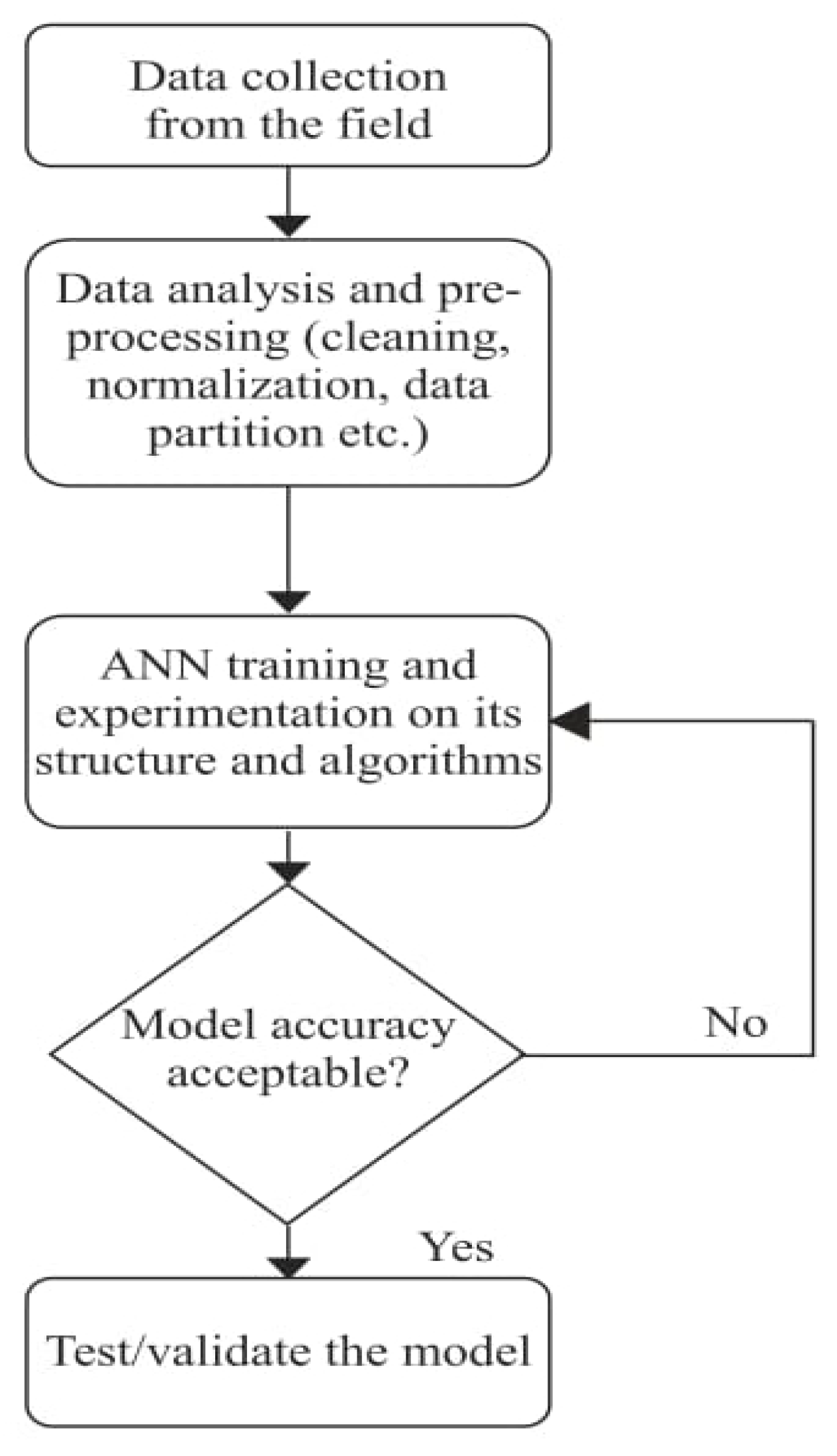
According to the summary listed in Table 2, some experimentation needs to be carried out to investigate various setups of the ANN model that will give the optimum prediction results. The first result is a related feature selection, as this is the first stage of data preparation before ANN training. The features were selected based on the correlation score between the independent variable (input features) and the dependent variable (target). Table 3 shows the correlation score for each feature and the target/output variable. The result indicates a strong correlation (R = 0.739) between weighted rainfall ( x 1 ) and the river flow ( y ). It can be concluded that the correlation between a min of temperature ( x 3 ) and the target variable ( y ) is very low and therefore x 3 was removed from the input feature. The lowly correlated feature would degrade the prediction accuracy if it was not removed from the feature.
With these four selected features (after removing x 3 ), the ANN training experimentation proceeds and the evaluation is performed. For the model parsimony reason, further removal of either feature x 4 or x 5 is also investigated to ascertain whether it affects the model accuracy. This is because these two features are of the same type, i.e., temperatures.
The first experimentation is mainly to investigate the number of hidden layer neurons and comparisons between FFNN and CFNN trained with the LM algorithm. Table 4 shows the results of this experimentation. The two numbers in the hidden layer neurons indicated that two hidden layers were used with the corresponding number of neurons in each layer. In the first column of Table 4, the notation in the square bracket indicates the number of hidden layer neurons, for example, [5] meaning there are 5 neurons in 1 layer, {10 + 10} meaning that there are 10 neurons in two hidden layers, etc.
The main finding in this experimentation is that the ANN trained with LM algorithm have a high tendency of overfitting, i.e., good prediction (even perfect, R 2 = 1 ) for training data but poor prediction of testing data. This occurs in both models using FFNN and CNNN structure. Some worse cases of this situation are highlighted in gray where the obtained RMSE is very high such that the ANN failed to make predictions, i.e., resulting negative values of R 2 , marked with ‘−’ in the Table. In addition, increasing the number of neurons (and layers) tends to increase the chance of overfitting.
The second experimentation is the same as the first, but the BR training algorithm was used. Table 5 shows the results of this experimentation. In Table 5, the lower RMSEs obtained during model testing are marked by ‘*’ and the overfitting situations are highlighted in gray. It can be seen from Table 5 that, generally, CFNN with one hidden layer (5 to 20 number of hidden neurons) sufficiently produced lower RMSEs when it is trained with BR algorithms. Moreover, the increasing number of neurons (and layers) did not give a satisfactory performance as can be seen from both Table 4 and Table 5. Especially for the FFNN, poor generalization capability (overfitting) was observed when the number of hidden neurons gets larger. During testing, the lowest RMSE of 211.1 was obtained when CFNN with 20 hidden neurons (1 layer) was trained with the BR algorithm.
The third experimentation was conducted to show the results of FFNN and CFNN training using the PSO algorithm (FFNNPSO and CFNNPSO respectively) where Clerc’s PSO version was used. The number of populations used in the PSO is set to 40, and the iteration number is set to 1000, the same as the one used in the LM and BR algorithms. The results are shown in Table 6. As compared to the previously trained ANN with LM and BR algorithm, both FFNN and CFNN trained with PSO (FFNNPSO and CFNNPSO) generally show good prediction ability in both the training and testing dataset, except for a few cases when two hidden layers are used (highlighted in gray). Therefore, it is preferable to use only one hidden layer to prevent overfitting. Thus, in the next experimentation, only one hidden layer was used with some variations in the number of neurons. The few lowest RMSE during testing were obtained (marked by ‘*’) for both FFNNPSO and CFNNPSO with 1 hidden layer, except for 1 case of FFNNPSO (row 5 of Table 6). In all experimentations with one hidden layer, only FFNNPSO with 10 hidden neurons shows slightly lower RMSE during the testing, as shown in row 2 of Table 6.
Furthermore, the fourth and fifth experimentation was conducted to investigate the CFNN model performance when only three features were used as the parsimonious model. The three features ( x 1 , x 2 , x 5 ) were used in the fourth experimentation, while another combination of three features ( x 1 , x 2 , x 4 ) were used in the fifth experimentation. The result of the fourth experimentation is shown in Table 7, where FFNNPSO and CFNNPSO with a different number of neurons in one hidden layer were investigated. The result indicates that it is possible to have a parsimonious model with only three features ( x 1 , x 2 , x 5 ) as the ANN input. The prediction on testing data gave the best performance of R 2 = 0.88 , R M S E = 191.1 cms and M P E = 0.09 % when CFNNPSO with 10 hidden neurons was trained despite slightly lower RMSE during the training as compared to the rest. This makes sense since the feature x 4 and x 5 are basically of the same type, i.e., mean and max temperatures, as compared to the result in Table 6 with four features. Similarly, the results obtained in this study corroborates with the work of Khaki et al. [35], who reported an R 2 value of 0.84 in the estimation of Langat Basin using a feed-forward neural network. Additionally, Hong and Hong [36] obtained R 2 values of 0.85, 0.81, and 0.85 for validation, training and testing datasets, respectively, when multi-layer perceptron neural network models were applied in estimating the water levels of Klang River.
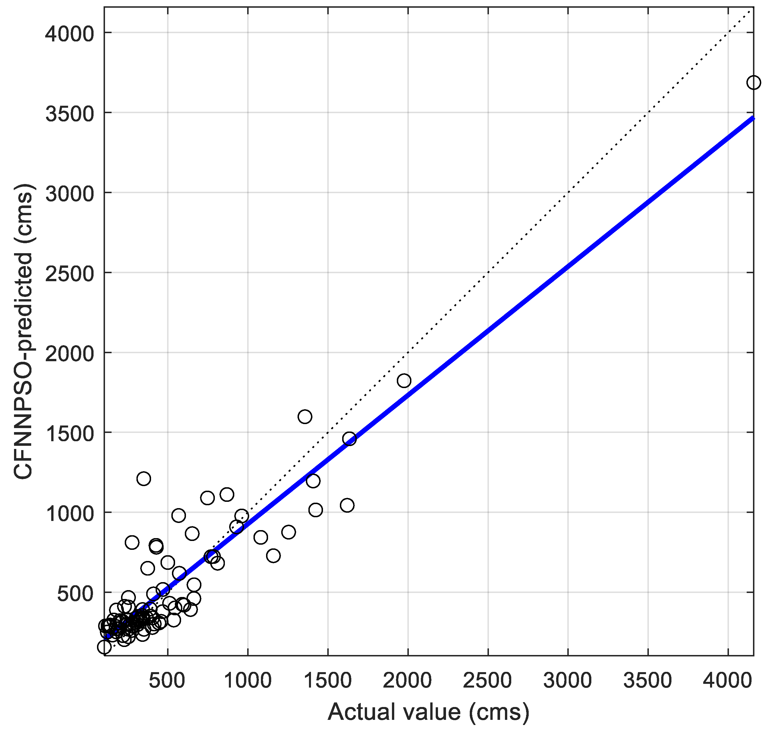
Figure 4 shows the regression plot of the best testing performance for CFNNPSO, with 10 hidden neurons (1 layer) and three input features ( x 1 , x 2 , x 5 ), resulting to R 2 = 0.88 , R M S E = 191.1 cms and M P E = 0.09 % .
Table 8 shows the results of the fifth experimentation using another three combinations of features ( x 1 , x 2 , x 4 ). However, the result shows quite significant degradation of the model performance, particularly with the training dataset. This means that the combination of the three features is not feasible to build a parsimonious predictive model. As the final remarks on the feature selection, the accurate model can be achieved using four features ( x 1 , x 2 , x 4 , x 5 ) or using three features ( x 1 , x 2 , x 5 ) as these two can achieve comparable performance as long as one hidden layer is used. In other words, ANNs trained with PSO were able to achieve acceptable accuracy in predicting river flow by using only weighted rainfall, average evaporation and max temperature as input variables. However, CFNN structure is generally preferable as this can produce more robust generalization performance despite the number of neurons applied.
Furthermore, as a comparison, Multiple Linear Regression (MLR) is also used to benchmark the prediction outcome of the ANNs above. The MLR is trained via Lasso regression/L1 [37] with the regularization parameter value ( α = 0.2 ) as the same one used during training using the BR algorithm. With the three features ( x 1 , x 2 , x 5 ), the resulting MLR prediction of the river flow can be expressed in the following equation:
y ^ = ( 2120.47 ) x 1 + ( 502.76 ) x 2 ( 1185.77 ) x 5 + 447.32
The MLR prediction on the test dataset produces a regression coefficient ( R 2 ) of 0.73 and an RMSE of 279.3 cms, which is lower accuracy compared to the FFNNPSO and CFNNPSO prediction. This makes sense since MLR assume linear relation on the variables.
Finally, the results of this study can be improved from the enhancement of data and improvement of the algorithm. Data-driven predictive modelling relies on the quantity and quality of the recorded data. Moreover, collection of field data is a costly practice that provides a series of snapshots of watercourse behaviour and supplements existing information. Therefore, it is essential to carry out a collaborative desk analysis to gather established existing records from different sources (consultants, environment agency or water services company) to improve current understanding and expertise deficiencies [38]. Additionally, hydrological and mathematical models play a significant role in the forecasting of river basins using field data obtained from different temporal and spatial scales [39].

4. Conclusions

Predictive modelling of river flow based on meteorological weather data using the Multilayer Artificial Neural Networks (ANNs) Particle Swarm Optimization (PSO) algorithm has been discussed. Sungai Kelantan river flow data ranging from January 1988 to December 2016 was used. The results demonstrate the potential applications of ANNs as an artificial intelligence-machine learning tool to predict river flow variables based on meteorological and weather data as studied in this paper, where two ANNs structures were used: feed-forward neural networks (FFNN) and cascade-forward neural networks (CFNN). The PSO algorithm used to train the ANN has also contributed to the advancement of the predictive model building. Generally, ANNs with one hidden layer trained using PSO were able to produce acceptable accuracy and good generalization for both the training and testing dataset. This result is better than the prediction performance of the Multiple Linear Regression (MLR) trained via Lasso Regression/L1. Moreover, a parsimonious model with reduced features was proposed; this feature was carefully selected. From the parsimonious model experimentation, it was possible to build an ANNs predictive model that can achieve acceptable accuracy in predicting river flow by using only weighted rainfall, average evaporation and max temperature as input variables. The experimentation results also indicate that CFNN trained using the PSO algorithm has more robust generalization performance compared to FFNN in the reduced feature (parsimonious) model. The model accuracy can still be improved using advanced techniques in machine learning modelling such as the ensemble method, improvement of the optimizer and cross-validation training procedure.
Furthermore, future research will work on some areas including benchmarking with other machine learning algorithms, benchmarking with other mete-heuristic algorithms for ANN training, data augmentation to enhance the diversity of the available data without generating actual data and real-time deployment of the predictive model in the Internet of Things (IoT) scenario. Despite the efficiency of ANNs as a black box model for river flow modelling, further exploration of research in this area is required. These include an automated feature selection mechanism, the possibility of using Deep learning neural networks regression, and improvement of accuracy to reduce overfitting via different optimizer algorithms. Another area includes the deployment stage of the machine learning model, which can involve Big Data, IoT and the Cloud computing platform. As AI tools in this regard are easily available nowadays, the area of this study promises high applicability of hydro-informatics systems, especially in Malaysia. This hydro-informatics concept and implementation need more extensive attention by authorities and decision makers to deal with water resource management which is currently a serious issue in some countries.

Author Contributions

Methodology, G.H. and M.I.S.; software, M.I.S.; validation, M.I.S., G.H. and H.M.M.; formal analysis, M.I.S. and G.H.; investigation, G.H., M.I.S., H.M.M.; resources, G.H.; data curation, G.H. and M.I.S.; writing—original draft preparation, G.H., M.I.S. and H.M.M.; writing—review and editing, G.H., M.I.S., H.M.M.; visualization, H.M.M.; supervision, G.H.; funding acquisition, G.H. All authors have read and agreed to the published version of the manuscript.

Funding

This research was funded by Universiti Tenaga Nasional (UNITEN) under the BOLD2020 grant.

Conflicts of Interest

The authors declare no conflict of interest.

References

  1. Hayder, G.; Kurniawan, I.; Mustafa, H.M. Implementation of Machine Learning Methods for Monitoring and Predicting Water Quality Parameters. Biointerface Res. Appl. Chem. 2020, 11, 9285–9295. [Google Scholar]
  2. Gorashi, F.; Abdullah, A. Prediction of water quality index using back propagation network algorithm. case study: Gombak river. J. Eng. Sci. Technol. 2012, 7, 447–461. [Google Scholar]
  3. Luo, P.; He, B.; Takara, K.; Razafindrabe, B.H.N.; Nover, D.; Yamashiki, Y. Spatiotemporal trend analysis of recent river water quality conditions in Japan. J. Environ. Monit. 2011, 13, 2819–2829. [Google Scholar] [CrossRef] [PubMed] [Green Version]
  4. Avvannavar, S.M.; Shrihari, S. Evaluation of water quality index for drinking purposes for river Netravathi, Mangalore, South India. Environ. Monit. Assess. 2008, 143, 279–290. [Google Scholar] [CrossRef]
  5. Dibike, Y.B.; Solomatine, D.P. River flow forecasting using artificial neural networks. Phys. Chem. Earth B Hydrol. Ocean. Atmos. 2001, 26, 1–7. [Google Scholar] [CrossRef]
  6. Mustafa, M.R.; Isa, M.; Bhuiyan, R. Prediction of River Suspended Sediment Load Using Radial Basis Function Neural Network-A Case Study in Malaysia. In Proceedings of the 2011 National Postgraduate Conference, Kuala Lumpur, Malaysia, 19–20 September 2011; pp. 1–4. [Google Scholar]
  7. Tengeleng, S.; Armand, N. Performance of using cascade forward back propagation neural networks for estimating rain parameters with rain drop size distribution. Atmosphere 2014, 5, 454–472. [Google Scholar] [CrossRef] [Green Version]
  8. Afan, H.A.; El-Shafie, A.; Yaseen, Z.M.; Hameed, M.M.; Wan Mohtar, W.H.M.; Hussain, A. ANN Based Sediment Prediction Model Utilizing Different Input Scenarios. Water Resour. Manag. 2014, 29, 1231–1245. [Google Scholar] [CrossRef]
  9. Memarian, H.; Balasundram, S.K. Comparison between Multi-Layer Perceptron and Radial Basis Function Networks for Sediment Load Estimation in a Tropical Watershed. J. Water Resour. Prot. 2012, 04, 870–876. [Google Scholar] [CrossRef]
  10. Uca; Toriman, E.; Jaafar, O.; Maru, R.; Arfan, A.; Ahmar, A.S. Daily Suspended Sediment Discharge Prediction Using Multiple Linear Regression and Artificial Neural Network. J. Phys. Conf. Ser. 2018, 954. [Google Scholar] [CrossRef] [Green Version]
  11. Mirjalili, S.; Mohd Hashim, S.Z.; Moradian Sardroudi, H. Training feedforward neural networks using hybrid particle swarm optimization and gravitational search algorithm. Appl. Math. Comput. 2012, 218, 11125–11137. [Google Scholar] [CrossRef]
  12. Wu, H.; Zhou, Y.; Luo, Q.; Basset, M.A. Training feedforward neural networks using symbiotic organisms search algorithm. Comput. Intell. Neurosci. 2016, 2016. [Google Scholar] [CrossRef] [PubMed]
  13. Tarkhaneh, O.; Shen, H. Training of feedforward neural networks for data classification using hybrid particle swarm optimization, Mantegna Lévy flight and neighborhood search. Heliyon 2019, 5. [Google Scholar] [CrossRef] [PubMed] [Green Version]
  14. Mirjalili, S. How effective is the Grey Wolf optimizer in training multi-layer perceptrons. Appl. Intell. 2015, 43, 150–161. [Google Scholar] [CrossRef]
  15. Xue, Y.; Tang, T.; Liu, A.X. Large-scale feedforward neural network optimization by a self-adaptive strategy and parameter based particle swarm optimization. IEEE Access 2019, 7, 52473–52483. [Google Scholar] [CrossRef]
  16. Yaghini, M.; Khoshraftar, M.M.; Fallahi, M. A hybrid algorithm for artificial neural network training. Eng. Appl. Artif. Intell. 2013, 26, 293–301. [Google Scholar] [CrossRef]
  17. Kulluk, S.; Ozbakir, L.; Baykasoglu, A. Training neural networks with harmony search algorithms for classification problems. Eng. Appl. Artif. Intell. 2012, 25, 11–19. [Google Scholar] [CrossRef]
  18. Pradhan, B.; Youssef, A.M. A 100-year maximum flood susceptibility mapping using integrated hydrological and hydrodynamic models: Kelantan River Corridor, Malaysia. J. Flood Risk Manag. 2011, 4, 189–202. [Google Scholar] [CrossRef]
  19. Nashwan, M.S.; Ismail, T.; Ahmed, K. Flood susceptibility assessment in Kelantan river basin using copula. Int. J. Eng. Technol. 2018, 7, 584–590. [Google Scholar] [CrossRef] [Green Version]
  20. Faisal, N.; Gaffar, A. Development of Pakistan’s New Area Weighted Rainfall Using Thiessen Polygon Method. Pak. J. Meteorol. 2012, 9, 107–116. [Google Scholar]
  21. Hsu, H.H.; Hsieh, C.W.; Lu, M. Da Hybrid feature selection by combining filters and wrappers. Expert Syst. Appl. 2011, 38, 8144–8150. [Google Scholar] [CrossRef]
  22. Vincent, W.; Winda, A.; Iwan Solihin, M. Intelligent Automatic V6 and V8 Engine Sound Detection Based on Artificial Neural Network. E3S Web Conf. 2019, 130, 01035. [Google Scholar] [CrossRef]
  23. Warsito, B.; Santoso, R.; Suparti; Yasin, H. Cascade Forward Neural Network for Time Series Prediction. J. Phys. Conf. Ser. 2018, 1025. [Google Scholar] [CrossRef]
  24. Anbazhagan, S.; Kumarappan, N. A neural network approach to day-ahead deregulated electricity market prices classification. Electr. Power Syst. Res. 2012, 86, 140–150. [Google Scholar] [CrossRef]
  25. Er, O.; Yumusak, N.; Temurtas, F. Chest diseases diagnosis using artificial neural networks. Expert Syst. Appl. 2010, 37, 7648–7655. [Google Scholar] [CrossRef]
  26. Hagan, M.T.; Menhaj, M.B. Training Feedforward Networks with the Marquardt Algorithm. IEEE Trans. Neural Netw. 1994, 5, 989–993. [Google Scholar] [CrossRef] [PubMed]
  27. Dan Foresee, F.; Hagan, M.T. Gauss-Newton approximation to bayesian learning. In Proceedings of the IEEE International Conference on Neural Networks—Conference Proceedings, Houston, TX, USA, 12 June 1997; Volume 3, pp. 1930–1935. [Google Scholar]
  28. Kennedy, J.; Eberhart, R. Particle swarm optimization. In Proceedings of the ICNN’95—International Conference on Neural Networks, Perth, WA, Australia, 27 November–1 December 1995; Volume 4, pp. 1942–1948. [Google Scholar]
  29. Lim, W.H.; Isa, N.A.M.; Tiang, S.S.; Tan, T.H.; Natarajan, E.; Wong, C.H.; Tang, J.R. A Self-Adaptive Topologically Connected-Based Particle Swarm Optimization. IEEE Access 2018, 6, 65347–65366. [Google Scholar] [CrossRef]
  30. Clerc, M.; Kennedy, J. The particle swarm-explosion, stability, and convergence in a multidimensional complex space. IEEE Trans. Evol. Comput. 2002, 6, 58–73. [Google Scholar] [CrossRef] [Green Version]
  31. Rumelhart, D.E.; Hinton, G.E.; Williams, R.J. Learning representations by back-propagating errors. Nature 1986, 323, 533–536. [Google Scholar] [CrossRef]
  32. MacKay, D.J.C. Bayesian Methods for Backpropagation Networks. In Models of Neural Networks III; Springer: New York, NY, USA, 1996; pp. 211–254. [Google Scholar]
  33. Lim, W.H.; Isa, N.A.M. Particle swarm optimization with increasing topology connectivity. Eng. Appl. Artif. Intell. 2014, 27, 80–102. [Google Scholar] [CrossRef]
  34. Pranava, G.; Prasad, P.V. Constriction Coefficient Particle Swarm Optimization for Economic Load Dispatch with valve point loading effects. In Proceedings of the 2013 International Conference of Power, Energy and Control (ICPEC), Sri Rangalatchum Dindigul, India, 6–8 February 2013; pp. 350–354. [Google Scholar] [CrossRef]
  35. Khaki, M.; Yusoff, I.; Islami; Hussin, N.H. Artificial neural network technique for modeling of groundwater level in Langat Basin, Malaysia. Sains Malaysiana 2016, 45, 19–28. [Google Scholar]
  36. Hong, J.L.; Hong, K. Flood Forecasting for Klang River at Kuala Lumpur using Artificial Neural Networks. Int. J. Hybrid Inf. Technol. 2016, 9, 39–60. [Google Scholar] [CrossRef]
  37. Tibshirani, R. Regression Shrinkage and Selection via the Lasso. J. R. Stat. Soc. Series B 1996, 58, 267–288. [Google Scholar] [CrossRef]
  38. WaPUG. River Modelling Guide; CIWEM: London, UK, 1998; pp. 1–38. [Google Scholar]
  39. Zhang, Z.; Zhang, Q.; Singh, V.P.; Shi, P. River flow modelling: Comparison of performance and evaluation of uncertainty using data-driven models and conceptual hydrological model. Stoch. Environ. Res. Risk Assess. 2018, 32, 2667–2682. [Google Scholar] [CrossRef]
Figure 1. (a) Peninsular Malaysia map, (b) Kelantan State, and (c) the study area (using QGIS©).
Applsci 10 08670 g001
Figure 2. Illustration of the cascade-forward neural network (CFNN) structure used in this study [7].
Applsci 10 08670 g002
Figure 3. Flowchart of the ANN-based model building process.
Applsci 10 08670 g003
Figure 4. The best testing performance for the cascade-forward neural networks trained with particle swarm optimization (CFNNPSO) model ( R 2 = 0.88 ).
Applsci 10 08670 g004
Table 1. Variables and their attributes.
Target VariableInput Variables (Features)
Name of VariableRiver Flow Weighted Rainfall Average Evaporation Min of Temperature Mean of Temperature Max of Temperature
UnitcmsMmmm°C°C°C
Notation y x 1 x 2 x 3 x 4 x 5
Duration1988–2016
LocationKuala Krai city downstream
Table 2. Artificial neural network (ANN)-based model setup.
ANN Model PropertiesExperimentation
Feature Input Selection To use all features or reduced features using correlation score
ANN structure/architectureTo use feed-forward and cascade-forward structure
Number of hidden layer and its neuronsTo use 1 or 2 hidden layers with 5, 10, or more neurons in each layer e.g., [ n 1 + n 2 ] means n 1 neurons in hidden layer 1 and n 2 neurons in hidden layer 2
Training algorithms To use Levenberg–Marquardt (LM), Bayesian Regularization (BR) and Particle Swarm Optimization (PSO)
Table 3. Correlation score for feature selection.
VariablesCorrelation Score (R)
x 1 y 0.739
x 2 y −0.544
x 3 y −0.222
x 4 y −0.563
x 5 y −0.662
Table 4. Results on ANN trained with 4 features ( x 1 , x 2 , x 4 , x 5 ) using the Levenberg–Marquardt (LM) algorithm.
#ANN StructureFFNNLMCFNNLM
TrainingTestingTrainingTesting
Hidden Layer NeuronsR2RMSER2RMSER2RMSER2RMSE
1{5}0.85143.50.60372.00.87133.00.39462.2
2{10}0.91115.0972.90.89124.8734.7
3{20}0.91110.4>10000.9492.8>1000
4{5 – 5}0.90116.70.48425.10.9399.2>1000
5{10 – 10}0.9762.1>10000.9851.6>1000
6{20 – 20}1.00>10001.00>1000
7{5 – 10}0.9493.4>10000.9672.8739.2
8{10 – 5}0.9490.3>10000.9672.8>1000
Table 5. Results on ANN trained with 4 features ( x 1 , x 2 , x 4 , x 5 ) using the Bayesian Regularization (BR) algorithm.
#ANN StructureFFNNBRCFNNBR
TrainingTestingTrainingTesting
Number of Hidden Layer NeuronsR2RMSER2RMSER2RMSER2RMSE
1{5}0.84152.40.33482.40.78174.80.87211.4 *
2{10}0.86138.70.43447.30.78174.80.87211.2 *
3{20}0.83154.20.38464.70.78174.80.87211.1 *
4{5 + 5}0.92107.50.00899.50.88132.30.69327.2
5{10 + 10}0.9676.30.14548.40.9769.2675.4
6{20 + 20}0.9849.90.60372.10.9850.10.44442.9
7{5 + 10}0.9396.60.34481.00.93101.80.14548.9
8{10 + 5}0.9398.70.00693.10.66218.60.73309.1
Table 6. Results on ANNs trained with 4 features ( x 1 , x 2 , x 4 , x 5 ) using the Particle Swarm Optimization (PSO) algorithm.
#ANN StructureFFNNPSOCFNNPSO
TrainingTestingTrainingTesting
Number of Hidden Layer NeuronsR2RMSER2RMSER2RMSER2RMSE
1{5}0.80171.20.87198.4 *0.80167.60.79249.6
2{10}0.81165.40.73284.30.80168.70.85208.4 *
3{20}0.81167.40.85213.2 *0.80169.50.86203.5 *
4{5 + 5}0.83157.30.80243.70.81165.60.75270.6
5{10 + 10}0.81166.20.85208.0 *0.81166.60.68307.3
6{20 + 20}0.82162.40.43412.80.79172.20.28462.1
7{5 + 10}0.80171.70.85213.90.81165.10.38429.2
8{10 + 5}0.83158.40.74279.30.81163.90.73284.3
Table 7. Results on FFNN and CFNN trained using PSO with 3 features ( x 1 , x 2 , x 5 ).
#Number of Hidden Layer NeuronsFFNNPSOCFNNPSO
TrainingTestingTrainingTesting
R2RMSER2RMSER2RMSER2RMSE
1{5}0.80171.40.87197.6 *0.80168.00.85209.4
2{10}0.80170.20.76268.30.77181.60.88191.1 *
3{15}0.80170.10.78254.20.80170.60.87198.8 *
4{20}0.78174.20.78254.70.78177.90.87199.5 *
Table 8. Results on FFNN and CFNN trained using PSO with 3 features ( x 1 , x 2 , x 4 ).
#ANN StructureFFNNPSOCFNNPSO
TrainingTestingTrainingTesting
Hidden Layer NeuronsR2RMSER2RMSER2RMSER2RMSE
1{5}0.74193.00.87199.7 *0.73198.30.85211.4 *
2{10}0.75188.20.71294.70.73197.80.79250.4
3{15}0.74193.10.76266.70.72199.20.81238.5
4{20}0.74191.80.85207.60.73196.10.82230.4
Publisher’s Note: MDPI stays neutral with regard to jurisdictional claims in published maps and institutional affiliations.

