Article

Explicit Modeling of Meteorological Explanatory Variables in Short-Term Forecasting of Maximum Ozone Concentrations via a Multiple Regression Time Series Framework

by
Sigfrido Iglesias-Gonzalez
1,
Maria E. Huertas-Bolanos
1,
Ivan Y. Hernandez-Paniagua
2 and
Alberto Mendoza
1,*
1
Escuela de Ingeniería y Ciencias, Tecnológico de Monterrey, Av. Eugenio Garza Sada 2501, Monterrey, Nuevo León 649489, Mexico
2
Centro de Ciencias de la Atmósfera, Universidad Nacional Autónoma de México, Circuito de la Investigación Científica S/N, C.U., Coyoacán, Ciudad de México 04510, Mexico
*
Author to whom correspondence should be addressed.
Atmosphere 2020, 11(12), 1304; https://doi.org/10.3390/atmos11121304
Submission received: 4 November 2020 / Revised: 28 November 2020 / Accepted: 30 November 2020 / Published: 1 December 2020
(This article belongs to the Section Atmospheric Techniques, Instruments, and Modeling)

Abstract

:
Statistical time series forecasting is a useful tool for predicting air pollutant concentrations in urban areas, especially in emerging economies, where the capacity to implement comprehensive air quality models is limited. In this study, a general multiple regression with seasonal autoregressive moving average errors model was estimated and implemented to forecast maximum ozone concentrations with a short time resolution: overnight, morning, afternoon and evening. In contrast to a number of short-term air quality time series forecasting applications, the model was designed to explicitly include the effects of meteorological variables on the ozone level as exogenous variables. As the application location, the model was constructed with data from five monitoring stations in the Monterrey Metropolitan Area of Mexico. The results show that, together with structural stochastic components, meteorological parameters have a significant contribution for obtaining reliable forecasts. The resulting model is an interpretable, useful and easily implementable model for forecasting ozone maxima. Moreover, it proved to be consistent with the general dynamics of ozone formation and provides a suitable platform for forecasting, showing similar or better performance compared to models in other existing studies.

1. Introduction

Forecasting is an integral and useful task for managing urban air quality. Since the 1970s, forecasting techniques and tools have been developed in response to the severe pollution episodes that occurred between 1930 and 1960 in diverse parts of the world, particularly in Europe and the United States of America. Empirical approaches and statistical models were the first techniques used to forecast spatio-temporal pollutant concentrations. Afterwards, between 1970 and 1990, 3D air quality models were developed and applied on urban, regional and global scales [1]. Comprehensive 3D photochemical models solve the mathematical equations that describe the chemical and physical dynamics of pollutants in the atmosphere [2]. As inputs, 3D air quality models require a large amount of reliable meteorological, geographical and emissions data. In addition, in order to be implemented, they require high computational capacity as well as specialized knowledge about atmospheric chemical reactions and physical processes. These factors make the setup, execution and operation of these comprehensive models for forecasting pollutant concentrations technically complicated in some urban areas, especially those located in countries with emerging economies. Therefore, simpler mathematical and statistical models are still widely used.
Tropospheric ozone (O3) is a greenhouse gas and a criteria air pollutant that often exceeds the air quality standards in many urban areas around the world [3]. It is a secondary pollutant formed by chemical reactions of nitrogen oxides (NOx) (NOx = NO + NO2) and volatile organic compounds (VOCs) in the presence of sunlight. Ozone production is highly dependent on the levels of chemical precursors and meteorological conditions. Several studies have explored the effect of meteorological parameters on O3 concentrations [4,5,6]. In general, O3 tends to increase with higher temperatures, which controls the chemical reaction rates associated with its production [7]. In contrast, increased wind speed is usually associated with decreasing O3 levels due to a dispersion effect. Similarly, increases in relative humidity are related to decreases in O3 because higher humidity levels are associated with greater cloud abundance and atmospheric instability [5]. Similarly, reductions in solar radiation are usually associated with reductions in O3 because its formation also depends on photochemical reactions. The complex, nonlinear process of O3 formation makes the short-term forecasting of O3 challenging, requiring sophisticated mathematical and statistical approaches.
Existing studies have reported a number of diverse mathematical approaches for forecasting ground-level O3 and other pollutants. Artificial Neural Networks (ANN) are the most common mathematical models that are used to forecast air pollution. Users of this approach emphasize its effectiveness when dealing with nonlinear systems [8,9,10,11,12,13,14]. However, ANN are commonly called “black box” models because of their limited capacity to provide information for interpreting the effect of the predictor variables on the output; they present generalization issues and are computationally intensive and time consuming compared to statistical models [15,16]. ANN are widely accepted, but they are more popular in applications where model interpretation is of secondary importance [17]. Less common mathematical approaches for forecasting ground-level O3 include Fuzzy Time Series (FTS) [16,18] and additive models [19].
Statistical models have also been widely used to forecast O3 concentrations and other criteria air pollutants. The Autoregressive Integrated Moving Average (ARIMA) model [20] is a classical modeling and forecasting technique that is widely used to analyze linear time series data. Multiple studies [21,22,23,24,25,26,27] have found that both ARIMA and ARMA models are reliable and capable of predicting short-term O3 concentrations. However, most of these studies have not included explicitly the effect of meteorological variables in predicting O3 concentrations, or the typical temporal resolution is not finer than a daily forecast. This latter characteristic makes some of the designed models inappropriate for use by environmental authorities that require to release O3 forecasts more than once during the day in order to limit the risk of human exposure to air pollution episodes. The few studies that apply ARIMA models to predict O3 concentrations with an explicit treatment of meteorological conditions with explanatory variables [25], tend to exclude the physical interpretation of the results. Other ARIMA models that consider heteroscedasticity show improvements in forecasting performance [28,29], but as in the aforementioned studies, they leave out meteorological information. Multiple linear regression (MLR) models are usually applied to assess the effect of meteorological conditions on O3 concentrations [30,31,32,33], but they are less commonly used to predict O3 concentrations. Wang [34] found that an ARMA model generally fits slightly better than MLR models when comparing the ability of the models to predict O3, CO (carbon monoxide) and NO2 (nitrogen dioxide) monthly maximum one-hour concentrations.
Studies that have compared statistical models with algorithmic techniques (i.e., ARIMA versus ANN) have not shown a single conclusive result regarding their capability to forecast air pollutants [28]. A frequent practice is to combine algorithmic and statistical models to produce hybrid models to forecast air pollution [15,35,36,37,38,39]. Overall, hybrid models are capable of accurately and precisely predicting pollutant concentrations. However, when the computational capacity is limited, hybrid models are not recommended.
In general, for the purposes of environmental authorities, forecasting models need to predict pollutant concentrations in real time, several times per day and over short time intervals after new data become available. Particularly, in emerging economies, it is important that forecasting models can be executed on platforms with low computational resources and that they are self-contained (without external sources of information other than the measurements available in the air quality monitoring network). In addition, the development of time series models with explanatory variables continues to be an active area of interest, in particular in the environmental sciences [40]. Considering these requirements, in this work, a general Multiple Regression with Seasonal Autoregressive Moving Average (SARMA) errors model was conceived and obtained to forecast maximum O3 concentrations, with a number of novel design and operational features. The model was implemented in the Monterrey Metropolitan Area (MMA) of Mexico and incorporates explicitly concurrent effects of meteorological variables (as exogenous variables) on the forecast O3 concentration and effects of past, recent and cyclic O3 concentrations. This approach enables a physical interpretation of the model. Furthermore, maximum O3 concentrations are forecast with a short time resolution: overnight, morning, afternoon and evening. In operational terms, the proposed modeling approach allows fast computation with moderate computational resources.

2. Description of the Application Urban Location

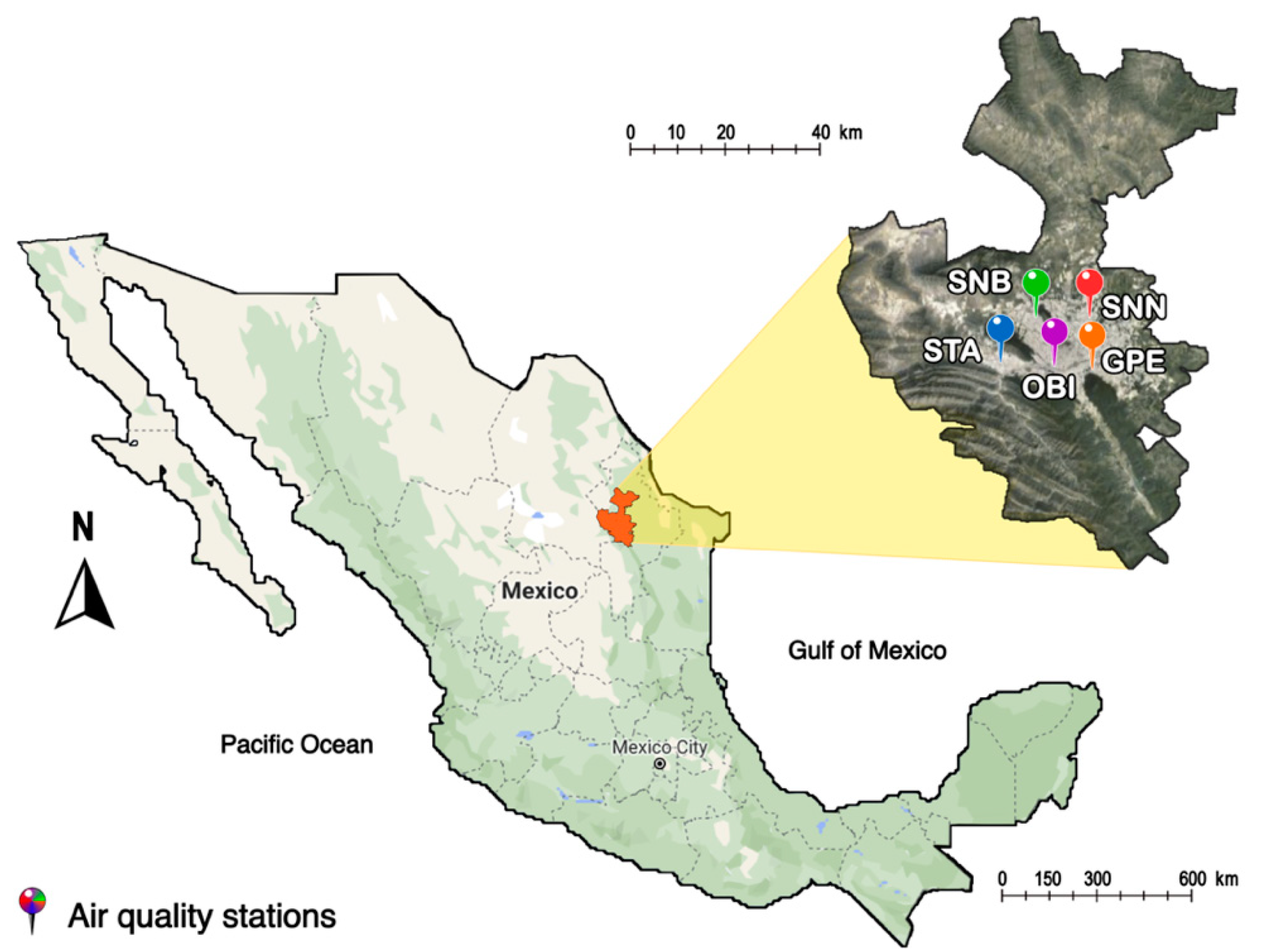
2.1. Geographical and Meteorological Characteristics

The MMA is located in the northeastern Mexican state of Nuevo Leon, surrounded by mountains to the south and west and flat terrain to the northeast, with an average altitude of 500 m a.s.l. (Figure 1). The MMA is the third most populated Mexican metropolitan area, comprising around 88% of the population of the State of Nuevo Leon, which corresponds to 4.1 million inhabitants [41]. In addition, it is the largest urban region in the north of Mexico, with around 1150 km2 of urbanized area and 14 municipalities [42]. The MMA makes the third largest contribution to Mexico’s GDP (7.5%, 2017) [43].
The climate of the MMA is semi-arid, and the meteorological conditions change substantially throughout the year. The annual average temperature is 20 °C, but the monthly average temperature ranges from 5 °C in January to 32 °C between May and August. August and September are the rainy months, and the annual average rainfall is about 650 mm [44].

2.2. Monitoring Network and Data

Within the MMA, the Integral Environmental Monitoring System (SIMA) started operating in November 1992 with five air quality monitoring stations. Subsequently, from 2009 to 2017, eight stations were progressively added to the air quality network. Today, SIMA operates thirteen sites, which have been monitoring tropospheric O3, six additional air pollutants (SO2, CO, NO2, NO, PM10, and PM2.5) and seven meteorological variables (temperature, solar radiation, relative humidity, rainfall, atmospheric pressure, wind speed and wind direction). In accordance with EPA EQOA-0880–047, from 1993 to 2003, UV photometric analyzers (Thermo Environmental Instruments Inc. (TEI), model 49) were used to measure O3 with a precision less than 2 ppbv and a detection limit of 2 ppbv. After May 2003, the TEI model 49 was replaced by model 49C, which has a precision better than 1 ppbv and a detection limit of 1 ppbv [45].
Ozone concentrations and meteorological variables are recorded every minute and summarized as hourly averages. These summaries were provided by SIMA from 2009 to 2016. Only five sites (OBI, GPE, SNB, SNN, STA) were selected to conduct the modeling, based on the following criteria: (i) the sites are the oldest of the SIMA, guaranteeing long data records, (ii) the selected sites had more than 75% data availability of O3 data and (iii) there was a lower proportion of outliers and inconsistent data compared to other monitoring sites. Table 1 briefly describes each of these selected monitoring sites.

2.3. Ozone Pollution in the MMA

Within the MMA, O3 concentrations frequently exceed the O3 one-hour average (110 ppbv) and the running eight-hour average (80 ppbv) national standards, making it the metropolitan area with the fourth highest O3 pollution levels in Mexico [46]. From 1993 to 2014, the air quality monitoring site that presented the largest number of exceedances was STA (on the west side of the basin), followed by the SNB, GPE and OBI sites. This is due to the fact that prevailing winds in this region are from east to west. In addition, the O3 concentrations have increased by 0.22 ppbv/year, showing the maxima during spring and minima in winter [45]. These conditions indicate that O3 is an air quality problem that needs to be addressed in the MMA. Previous O3 studies conducted in the MMA indicate that there is an observable relation between O3 and certain meteorological variables (solar radiation, temperature and wind direction) [45,47]. However, the methodologies presented in those studies do not explicitly model O3 as a function of those meteorological variables. Furthermore, Carrillo-Torres et al. [47] found that the seasonal cycles of O3 are mainly governed by changes in meteorology more than by primary emissions. This implies that understanding the effect of meteorological variables on O3 concentrations is important for predicting possible pollution episodes in the MMA, as in other urban centers.

3. Methods

3.1. Data Processing

Daily six-hour maximum O3 concentrations were computed four times each day: overnight, morning, afternoon and evening. The time frame according to which the calculations were made is shown in Table 2. Under this arrangement, the computation and availability of forecasts is made at 05:00, 11:00, 17:00 and 23:00 Central Standard Time (CST) and at 06:00, 12:00, 18:00 and 00:00 daylight saving time (DST).
Because each time of the day is represented by a single O3 maximum value, which may occur at any, non-fixed time within the six-hour interval, it is necessary to have a summary measure of the meteorological predictors for such intervals. A weighted average of the meteorological values was computed for each time of day. The weights were determined by the relative frequency of the times for each hour in which the maximum O3 concentration is observed. Different weights are calculated for each site (Table 3). The weighted average wind direction was calculated using the vectorial cosine--sine representation.
The meteorological and O3 time series data were pre-processed to remove values outside of the admissible range and inconsistent recordings (special codings and sudden changes of scale). Missing data were estimated at a one-hour time scale using the Kalman Filter (KF) [48,49]. The KF is an algorithm that is widely used in time series analysis, allowing the computation of estimating functions, forecasts and interpolation of the series. When the filter is used for interpolation, it is usually called the Kalman Smoother (KS). In this setting, the filter interpolates observed values to fill in the missing data (imputation), provided a model for the series. If the series is governed by a Gaussian process, the imputed values are optimal, (i.e., unbiased and with minimum variance). In general, large autoregressive models of varying orders and regressors, such as time of the day, hour or month of the year, depending on the site were fitted on the hourly series, according to the scheme presented in Section 3.2. The KS was implemented in an iterative convergent way, in which an estimated MLR with AR errors model was used to impute the missing values and was then re-estimated for re-imputation and so on, until a convergence criterion was met (<10−6 for the norm of the differences of parameter estimates between iterations). A similar approach was taken for the meteorological variables.
In particular, the STA and OBI sites exhibited aberrant temperature recordings during 2012, inconsistent with the recordings observed for the other sites. Given the importance of temperature in forecasting O3 concentrations, the series data for 2012 were removed and estimated employing a regression model with correlated errors that used temperature records from the remaining sites as predictors along with the KS. From 2009 to 2011, solar radiation recordings were not available at the STA, SNB and SNN sites. Additionally, there were large data gaps for SNN in many meteorological variables up to May 2012. The forecasting models for the STA and SNB sites were thus estimated using information only from January 2012 onward, while estimation for the SNN site proceeded using data from June 2012 onward.
The sample used for estimation of the models is given in Table 4, which provides the total number of hourly observations employed for each site and the number of maxima O3 concentrations per time of day being modeled; dates are also indicated. Summary measures of maximum ozone concentrations are presented in Table 5. There are highly comparable averages (33.10 ppbv to 38.12 ppbv) and dispersion values (18.78 ppbv to 22.35 ppbv standard deviations) among sites. The computations shown here and those described in the following sections, including model fitting and forecast computation, were carried with R software, version 3.2.1. [50] using base packages only. For the construction of scatterplots (Figure 2), the hexbin package was employed.

3.2. General Statistical Approach

The employed modeling approach involves making use of meteorological variables together with past ozone concentrations as predictors. We consider the concurrent meteorological summary values (see Section 3.1) for the six-hour interval ozone concentrations being predicted as linear regressors in a multiple regression model. In this setting, the meteorological features are considered exogenous variables and define a mean level for ozone maximum concentrations according to the specific values that the variables assume at each interval. In this sense, the meteorological values are considered as given. Ozone departures from this mean level are treated as random deviations with a temporal structure (i.e., as a stochastic process), which can be exploited to predict current deviations from past values. This is accomplished through the family of S MMA models. The framework combining these considerations is known as the multiple linear regression model with SARMA errors. Seasonal effects, such as daily cycles, may also be included in either the regression part or the structural part of the model.
Six appropriately transformed meteorological variables were used as regression predictors: temperature (TEMP, °C), relative humidity (RH, %), solar radiation (SR, kW/m2), angular wind direction (WD, degrees) and wind speed (WS, km/h). The transformations were computed in order to linearize the relation with maximum O3 levels (see Section 3.4). Additionally, terrestrial rotation and translation effects were included in the regression model through the inclusion of time of day and month of the year as predictors. The baseline is the average January overnight level; every other month or time of the day effects represent deviations from this baseline. Note that a large number of degrees of freedom is available for the model estimation, as a total of 23 meteorological parameters plus six SARMA parameters were fit to the data based, at least, on 2920 observations (Table 4).
The predictive structure of the series is shown by the autocorrelation function (ACF) and the partial ACF (PACF) (correlations and partial correlations of present values with lagged values). We call the (partial) autocorrelations functions calculated from the observations the empirical (P)ACF.
These are the main tools that are commonly employed to identify a suitable model for stochastic dependence in ARMA modeling. Moreover, by simulating from an estimated candidate model and calculating its corresponding (P)ACF, a comparison with the empirical P(ACF) provides a valuable guide for assessing a proposed model, as the simulated (P)ACF of plausible models is expected to resemble the empirical (P)ACF of the series being considered.
We use the Box–Jenkins approach [20] for building a time series model, whose general steps are as follows:
  • Calculation of residuals from a multiple regression model with transformed meteorological predictors.
  • Identification of a SARMA model for the residuals via the ACF and PACF.
  • Model fitting, in which meteorological effects and SARMA parameters are simultaneously estimated.
  • Model diagnostic using Ljung-Box goodness of fit tests [51] and a comparison of empirical (P)ACF with the (P)ACF obtained by simulating from the fitted model.
  • Model selection based on the previous two steps.
The last three steps of the process are usually made in an iterative manner until a satisfactory model is obtained. Model selection is accomplished by combining Ljung–Box tests and empirical versus simulated (P)ACFs comparisons, aiming for a compromise between both criteria. Ljung–Box tests are a commonly used diagnostic tool that examine the autocorrelations of the model residuals at each lag. The tests check whether at least one autocorrelation at each or previous lags is significantly different from zero. Statistically significant (p-value ≤ 0.05) non-zero autocorrelations are indicative of model inadequacy.

3.3. The SARMA Model

A multiple regression model with multiplicative SARMA (p,q)(P,Q)s errors may be formulated as follows:
фp(B) ΦP(Bs) (ytxtβ) = θq(B) ΘQ(Bs)at
where yt and xt represent the O3 maxima and associated weighted average values of meteorological variables at time of day t, respectively; фp(B) = 1 − ф1B − … − фpBp, with Bpyt = ytp being an autoregressive operator of order p and θq(B) = 1 − θ1B − … − θqBq being the moving average operator for the regular part, respectively; ΦP(Bs) = 1 − Φ1Bs − … − ΦPBs+P is the autoregressive operator of order P, with s being the number of periods per season, and ΘQ(Bs) = 1 − Θ1Bs − … − ΘQBs+Q is the moving average operator of order Q for the seasonal part, respectively; at is usually assumed to be normal white noise with variance σ2a. For the series being modeled, s is expected to be equal to four (i.e., a daily cycle effect). The effect of meteorological variables on the maximum O3 concentration is represented by β.
The method of parameter estimation (ф, Φ, θ, Θ, β, σ2a) employed here is maximum likelihood estimation using the exact likelihood. Because of the assumptions made about at, the resulting probability distribution function for the process yt is Gaussian. Maximum likelihood estimates are the parameter values that maximize (1). Evaluation of the exact likelihood with state-space representations is given in [52] (p. 385); see also [20] (p. 243) for other approaches. For computational details, see [53]. Note that, for a forecast to actually be computed, parameter estimates are needed; we simply denote this forecast by y ^ t in the sequel.

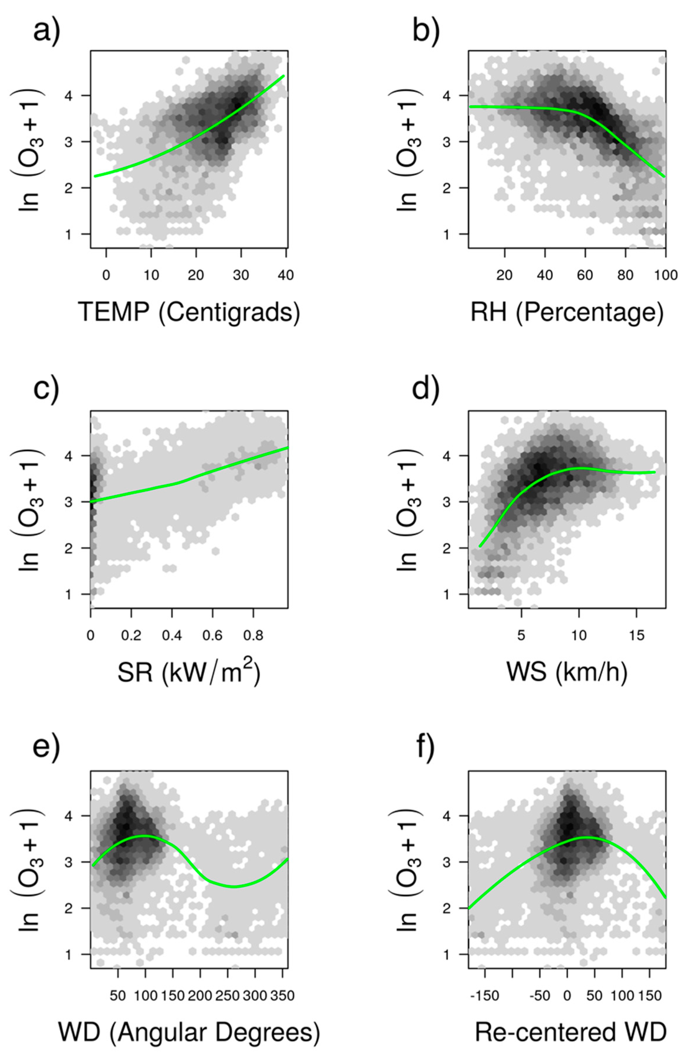
3.4. Meteorological Variables Transformations

Figure 2 shows scatterplots of the natural logarithm of maximum O3 concentrations and the weighted averages of meteorological variables at the OBI site (similar patterns are found at the other sites, and their plots are thus omitted in this section; see Figures S1–S5 in the Supplementary Material). A great deal of dispersion can be seen in the plots. The locally estimated scatterplot smoothing (LOESS) class of local regression models [54] is used in an ad hoc way as an aid to visualize local trends in the relationship between O3 maxima and the meteorological variables. The relationships in many cases are non-linear because meteorological variables are linked with direct and indirect effects in O3 concentrations [55,56,57,58]. The cyclic nature of angular WD explains the particular pattern between O3 concentrations and WD. Higher O3 concentrations are recorded when WD takes values between 60 and 120 degrees (north-east, east and south-east directions). This pattern can likely be explained by the fact that there is downwind transport in the MMA of photochemical air masses that come from the industrial sector located in these directions [45].
Proper modeling of these non-linear relationships through linear regression must make use of transformations of the meteorological variables. In general, graphical displays are employed to suggest suitable transformations. Commonly employed transformations in statistical regression analysis, such as natural logarithmic, polynomial and reciprocal functions, were applied to the meteorological variables. Note that the aim of these transformations is to capture the general underlying relationship between O3 concentrations and the meteorological variables and not to reproduce the fit given by the local regression, which is used here purely as an indicator of such a relationship.
Table 6 presents the formulas of the transformations used for each meteorological variable. Since there is a slight departure form linearity between TEMP and O3, a natural logarithmic transformation on TEMP was employed. For the slight curvature shown in the SR, a second-order polynomial was p proposed and found statistically significant (details are provided in Section 4.1). For RH, a third-order polynomial was employed. For WS, we used a reciprocal transformation, to resemble the asymptotic level reached by the dispersion effect of WS on O3 concentrations. WD has a cyclic relation to O3. We chose to re-center at the angle where the peak O3 concentration occurs and then model the deviation from this angle; as WD deviates from this angle, O3 concentrations decay. Therefore, we re-center angular WD for each site by computing its sine and cosine coordinates and rotating them counterclockwise by a specified angle; finally, we recover the WD in terms of “new” angles. Table 7 lists the angles selected for the rotation at each site. The other sites showed patterns similar to these, and the same formulas were employed.
Angular WD was further transformed using
xI(0 ≤ x ≤ 180) + |x − 360|I(360 > x > 180)
where x is the angular direction in the new coordinates (after rotation), and I is an indicator variable, which takes values 0 or 1 according to whether the variable is in the interval between in parentheses. The formula therefore restricts x values to lie within 0 and 180 as WD departs from the new center.

3.5. Performance Measures

Forecast performance measures are usually employed to assess the ability of a given model to forecast the time series. Table 8 lists the definitions and meanings of the measures used in this study; the notation y ^ t denotes the one-step-ahead forecast at time of day (six-hour interval) t computed from information up to time t−1 (all relevant previous information). These measures should be close to zero for a good forecasting procedure.
Computation of these measures is performed using the sample estimation period (see Section 3.1) and two-week left-out sample (observations not used in model estimation), separately. In the latter period, observed meteorological information was used. Comparison of the performances in both periods provides an indication of how well the estimated model captures the data-generating process and thus offers an assessment of its capacity to produce good-quality forecasts.

4. Statistical Analysis and Results

4.1. Model Estimation

A SARMA (3,0) (3,0)4 single general model was found to account equally well for the maximum O3 time series structure for every site. Figure 3 shows the empirical (P)ACF computed from the historical observations and the simulated (P)ACF computed from this model for the OBI site series only. The remaining sites behave virtually in the same manner. The plot exhibits a typical exponential decay of ACF for both the regular and the seasonal component together with the corresponding cutoffs of (P)ACF at the first few lags, which is common in autoregressive models. The seasonal period is of order four, representing a day-period effect. No lack of stationarity is evident from the (P)ACF plots.
Parameter estimates of the fitted models are given in Table 9. The estimates of the ARMA model are shown first, and the remaining ones are the estimated regression coefficients. All first- and third-order regular autoregressive effects were significant (p 0.05). Furthermore, every effect describing the seasonal component was significant, except for the STA site. The first-order effects in both the regular and seasonal part present the largest magnitudes. Thus, the model recovers the effect of the previous time of day and a daily seasonal effect.
Table 9 shows significant increasing effects occurring mainly during springtime (March, April and May), while during the summer there is a decrease in O3 concentrations compared to the baseline, which probably is due to the fact that the highest wind speeds (>10 km h−1) are recorded during this time [45], promoting O3 dispersion. In contrast, December presents decreasing deviations in most sites because of reduced TEMP and SR. Other monthly deviations vary from site to site, but they are negligible or not statistically significant.
As for time of day effects, significantly increased deviations in O3 concentrations are observed between 12:00 and 17:00 CST. This is consistent with the enhanced photochemical period, in which O3 generally peaks in the MMA [45], and with the general O3 production dynamics during the day. The decreasing effects from the overnight baseline at any time of day for the OBI site might be explained by variables such as SR, TEMP and RH, whose influence on O3 formation mediates the time of day effect. The influence of meteorological variations is verified by the overall significant effect of their transformations exhibited in Table 9.

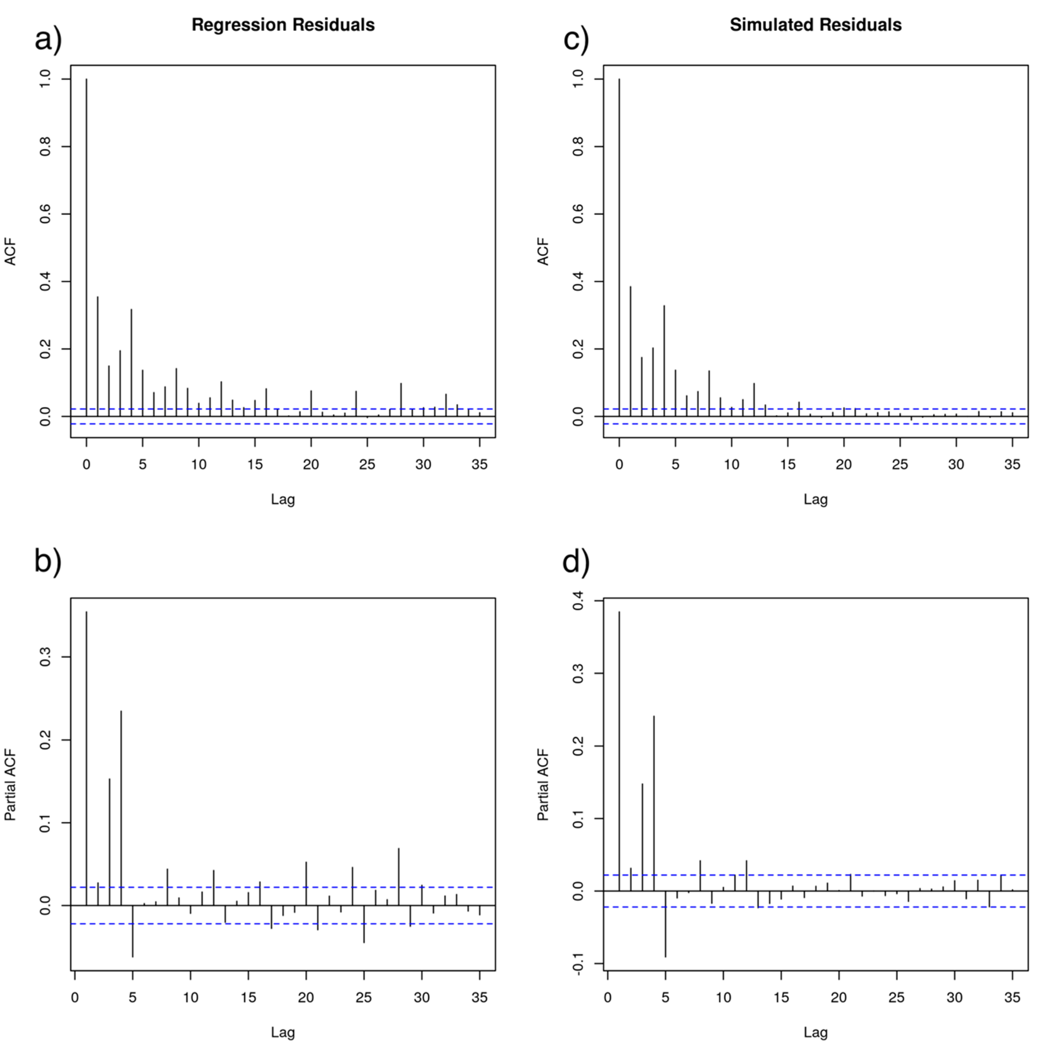
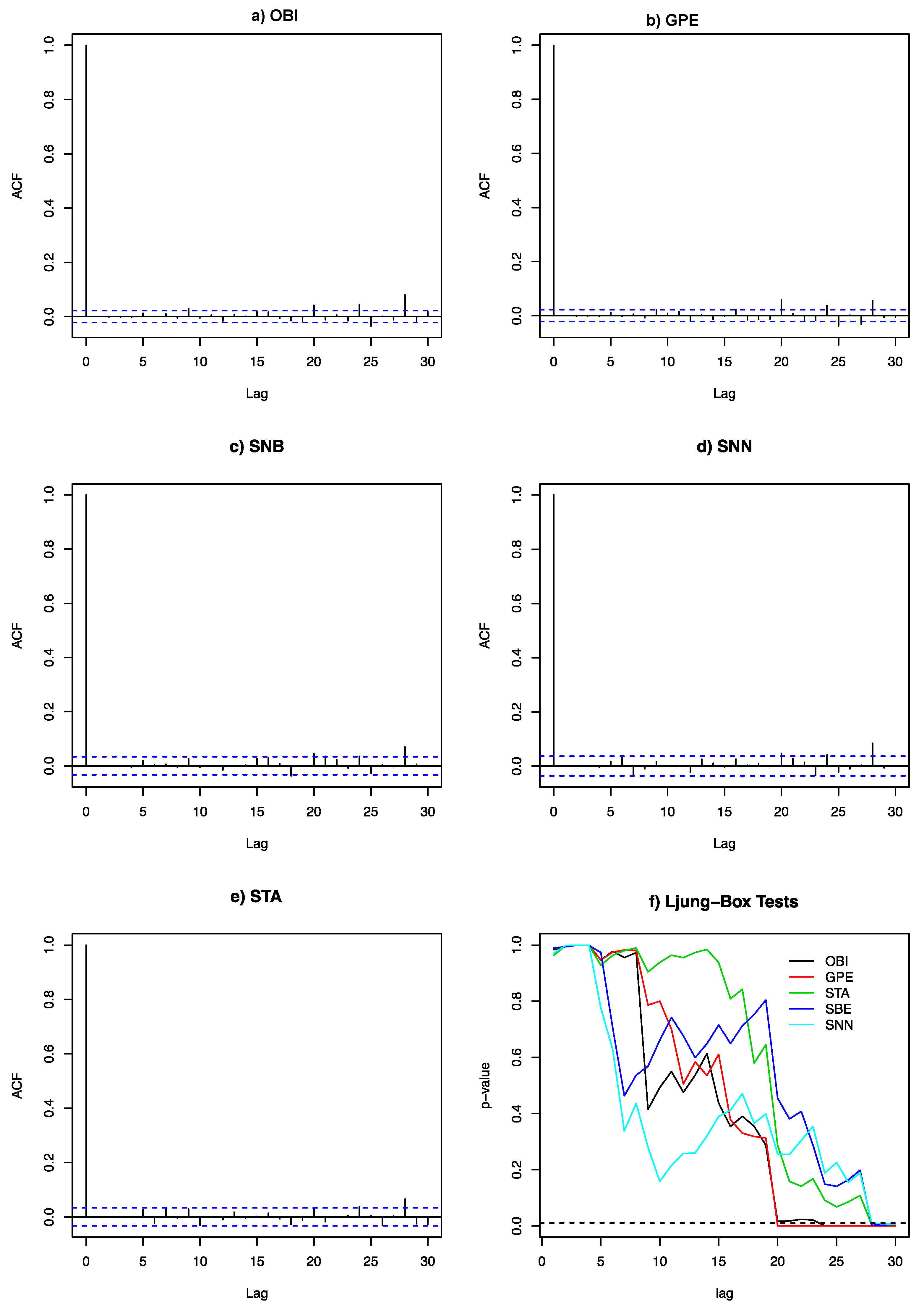
4.2. Model Diagnostics

A two-way assessment of the model is given by comparing the empirical versus simulated (P)ACF and the usual Ljung–Box tests. A plausible estimated model is expected to reproduce the empirical (P)ACF. This can be verified by simulating from the estimated model and calculating the (P)ACF from the simulated series. Figure 3 shows very similar (P)ACF patterns between the empirical and simulated series for the OBI site at recent previous times of day and discrepancies at larger lags corresponding to seasonal effects. No ARMA model with an increased number of lags for the seasonal part achieved a (P)ACF pattern similar to the empirical P(ACF). The remaining sites exhibited similar patterns.
ACF of residuals and Ljung–Box goodness of fit tests p-values are shown in Figure 4. Each lag represents a six-hour time interval. Larger lags ( 20) show statistically significant ACF, indicating model inadequacy; however, ACF magnitudes at those lags are rather small, representing marginal, 5–7 former days effects on O3 concentrations. The model accounts well for the immediately previous six-hour lags and daily cycles effects. Other models including moving average terms for both the regular and the seasonal component were not found to improve the fit. Overall, the set of tests performed appear to support an adequate good model fit.
Figure S6 in the Supplementary Material shows a further examination of residuals. A lack of constant variance is apparent in every site, as time intervals with different variability were observed. This represents a departure from the statistical model assumptions and deserves further investigation. For the purposes of this paper, we consider that the insights and forecasts provided by the model presented are reasonable, and accounting for variance heterogeneity may be regarded as a refinement of the original model. Thus, it can be said that the model adequately represents series behavior at recent times of the day, in which most of the predictive structure is available, and the remaining predictive structure of distant former days is negligible.

5. Forecast Performance
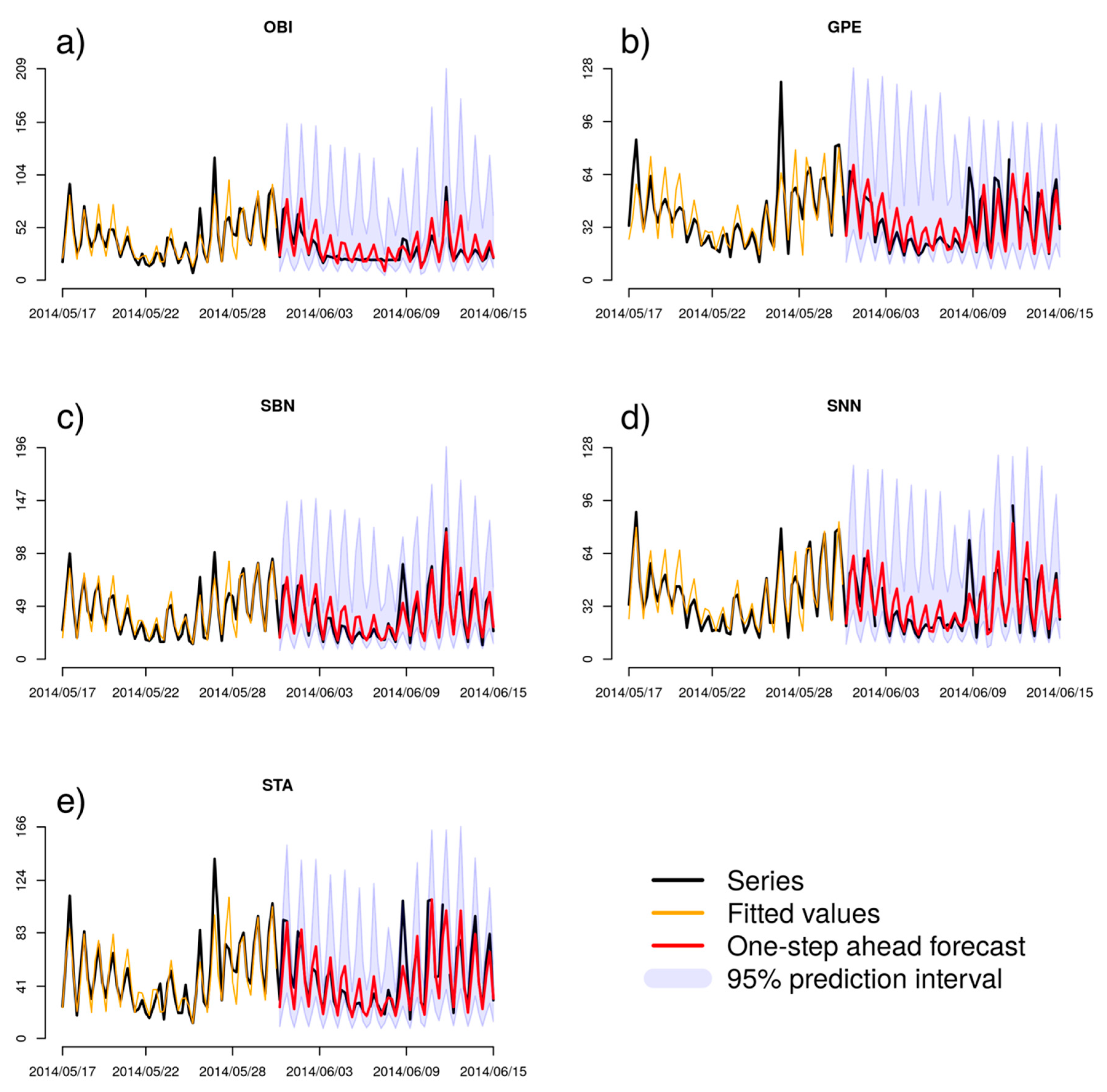
5.1. Results

Table 10 shows the performance measures assessing the fitted values of the estimated models, i.e., one-step-ahead forecasts computed using the estimation periods shown in Table 4. The fitted values were computed with a natural logarithmic scale, and then, inverse transformation was applied to allow comparison with the original untransformed maximum O3 level, through the performance measures presented in Section 3.5. Every performance measure was then computed with the original scale (ppbv).
Table 10 shows RMSE values around 10 units, ranging from 9.58 to 10.89. On average, the forecast error ranges from 6.87 to 8.15 in absolute value (MAE). As for the MAPE, it tends to exhibit the largest values, ranging from 25.65 to 32.31. Furthermore, the model tends to overestimate the maximum O3 concentrations, as every MPE is negative, around 8, with great variability among sites. NME values are around 21 and are similar among sites. Note that the site SNN consistently shows the best performance values, suggesting that this site is where the model fits better. The measures, however, are comparable between sites, and we may conclude that the model performs similarly for all of them, especially regarding the MAE and RMSE.
Table 11 shows the performance measures obtained using an out-of-sample period of days following the estimation period. Note that the performance measures are generally quite comparable to those from the estimation period listed in Table 10. During this out-of-sample period, the forecasts tend to overestimate the maximum O3 concentration, except for STA, which shows a positive MPE value. Figure 5 provides an illustration of the one-step-ahead forecast performance together with 95% prediction intervals in the last two weeks used for estimation and the following two weeks of left-out observations. Comparing both periods, we see similar forecast performances. We might conclude that the forecast performance does not decay when forecasting new observations not previously used for model fitting, and thus the model captures the processes behind the ozone records and provides a suitable framework for forecasting.

5.2. Comparison with Other Studies

Most of the existing studies that have reported AR(I)MA models generally do not consider meteorological variables for O3 prediction. There are a number of difficulties in comparing the results of this paper with those of other works. The different temporal resolutions used in the analyses, which range from hourly to monthly periods, the out-of-sample period, and the summary statistic that are reported do not allow a direct comparison with our models and forecasts. Thus, caution is needed in comparing and interpreting the performance measures. Kumar et al. [21] forecasted one-hour daily maximum O3 concentrations using an ARIMA (1,0,1) model, finding an RMSE of 9.55 and a MAE of 8.36, while Kumar and Jain [23] forecasted daily average O3 concentrations with an ARIMA (0,0,1) model and found an RMSE of 15.1 and a MAE of 10.9. Duenas et al. [22] built an ARIMA (1,0,0)(1,0,1)24 for hourly periods (O3 averages), showing a MAE of 10.62 and 5.96 in urban and rural areas, respectively. In contrast, Beldjillali et al. [26] found a MAE of 2.03 forecasting monthly average O3 concentrations with a simple model AR(1). In the present study, in which four maximum O3 concentrations per day are modeled, the models show RMSEs around 10 units and MAEs around 7 units for every site. Kumar et al. [21] and Kumar and Jain [23] showed MAPE values of 13.14 (daily maxima) and 25.8 (daily average), respectively. Duenas et al. [22], in the aforementioned work, found an MPE of −11.33 in urban areas. The SARMA models in the present study show MAPEs ranging between 19.50 and 25.65 and MPEs ranging between −3.09 and −14.03, depending on the site.
As mentioned, a direct comparison is difficult, especially regarding absolute measures such as RMSE and MAE; lower RMSE and MAE are expected for an adequate forecasting model at lower temporal resolutions when compared to higher-resolution modeling because of the smaller variability expected at lower resolutions. The present work shows similar RMSE and MAE measures to those presented in the reviewed papers; however, the temporal resolution presented here is higher. Although we may conclude that the models proposed here have better performance, the inherent variability of the data for the particular sites considered in the papers also prevents clear-cut comparisons. Perhaps MPE and MAPE are more comparable since they represent relative measures. In the present paper, MAPE tends to be larger than in the reviewed papers, and MPEs are negative (as the one discussed in the previous paragraph). It is worth noting that the magnitudes of these measures are similar. However, because temporal resolutions have an impact, both measures might increase since O3 concentrations at overnight times tend to be small. Finally, we conclude that the performance measures presented here are similar or better than the ones reported in other studies, presuming that the inherent variabilities of the studied data are comparable. The increase of MAPE in this paper is expected, as a higher temporal resolution is considered.
The use of 3D numerical air quality models is recommended to forecast air quality pollutants, as they are sophisticated tools that address the non-linearity of the photochemical system and include meteorological, terrain and emissions information to simulate pollutant dispersion [59]. Zhang et al. [1] reviewed the history and current status of 3D real-time air quality forecasting models, showing that they have been mainly used in the US and Europe. In the US, 3D forecasting models applied to predict eight-hour maximum hourly averages showed NME values between 17.0 and 30.4, averaging 23.9, and RSME values ranging from 8.7 to 31.0, averaging 16.0. In comparison, our study, which uses a six-hour resolution, shows NME values ranging from 20.6 to 23.6 and from 21.2 to 25.7 in the estimation and out-of-sample periods, respectively, which are well within the ranges of values and below or close to the average value of the 3D models discussed above. Regarding the RSME, our analysis achieves a maximum value of 14.6, combining both periods, which is less than the average value of the 3D models. Similar results were found in Catalonia in north-east Spain using the MM5/MNEQA/CMAQ modeling forecast system to predict eight-hour maximum O3 concentrations, with an RSME of 16.1, MPE of 1.1, MAPE of 13.3 and NME of 14.5 [60].
Other 3D air quality studies employed time resolutions less comparable to the one used in the present study. For example, Chai et al. [61] reported monthly and annual average O3 concentrations over the US applying the Eta/CMAQ system. Curier et al. [62] forecasted daily maximum O3 concentrations over Europe with the LOTOS-EUROS chemical transport model, and the CALIOPE modeling system (WRF-ARW/HERMES/CMAQ/BSD-DREAM8b) was applied over Spain to forecast one-hour O3 concentrations [63]. The values of the performance measures presented in these papers are similar to those discussed in the previous paragraph; however, the summaries employed for O3 concentrations and different time resolutions make detailed comparisons difficult. A common issue in some studies [1,63] is a tendency to overestimate O3 concentrations, just as the SARMA models presented here. Overall, the statistical models proposed in this study exhibit forecast performance comparable to that of 3D air quality systems, but with the use of low computational resources.

6. Conclusions

A univariate multiple regression model with meteorological predictors and SARMA errors has proven to be useful for representing the dynamics of O3 maxima at four times of the day (overnight, morning, afternoon and evening) in five sites of the MMA monitoring network in Mexico. The nonlinear nature of the relationship between O3 maxima concentrations and the meteorological variables can be easily transformed, making it amenable to linear modeling. A relevant contribution of this paper is the extension of the Box-Jenkins approach, which is commonly employed in the forecasting literature on O3 concentrations. Typically, this type of research has focused on building “pure” ARIMA models with no inclusion of additional predictors, while an important feature of the ARIMA methodology is its flexibility to incorporate external information into the model. We make use of meteorological predictors and prove their usefulness in understanding and forecasting maximum O3 concentrations with an adequate level of precision.
The quality of the statistical forecasts presented here can be considered good. Moreover, they are very similar to those obtained by 3D air quality systems and are computable with much less infrastructure, mathematical complexity and computational effort. Comparison with other studies using statistical models is difficult because of the specifics of each analysis; however, our forecasts are quite comparable and can be considered satisfactory. Overall, we conclude that the regression model with SARMA errors presented here recovers the general formation of O3 dynamics, reflecting the specifics of the MMA and providing good-quality forecasts. There is room for further analytical work within the developed framework. The model constitutes a foundation upon which additional refinements could be implemented to improve forecasting or to extend understanding of O3 dynamics in the MMA, with special attention to volatility features not addressed by the model. Future research could include the addition of O3 precursors concentrations as well as the concentration of other criteria pollutants as predictors, as well as other meteorological or anthropogenic drivers.

Supplementary Materials

The following are available online at https://www.mdpi.com/2073-4433/11/12/1304/s1, Figure S1: Relationship between natural logarithm of O3 and temperature (TEMP) for four sites in the MMA, Figure S2: Relationship between natural logarithm of O3 and relative humidity (RH) for four sites in the MMA, Figure S3. Relationship between natural logarithm of O3 and solar radiation (SR) for four sites in the MMA, Figure S4: Relationship between natural logarithm of O3 and wind direction (WD) for four sites in the MMA, Figure S5: Relationship between natural logarithm of O3 and wind speed (Ws) for four sites in the MMA, Figure S6: Residuals of estimated models at the natural logarithmic scale. Time intervals with different variabilities are observed for all sites.

Author Contributions

Conceptualization, A.M.; methodology, S.I.-G. and I.Y.H.-P.; software, S.I.-G.; validation, S.I.-G. and I.Y.H.-P.; formal analysis, S.I.-G.; investigation, S.I.-G., M.E.H.-B., I.Y.H.-P. and A.M.; resources, A.M.; data curation, S.I.-G. and I.Y.H.-P.; writing—original draft preparation, S.I.-G. and M.E.H.-B.; writing—review and editing, S.I.-G., M.E.H.-B., I.Y.H.-P. and A.M; visualization, S.I.-G. and M.E.H.-B..; supervision, A.M.; project administration, A.M.; funding acquisition, A.M. All authors have read and agreed to the published version of the manuscript.

Funding

This research received no external funding.

Acknowledgments

The authors would like to acknowledge the support of the Secretariat for Sustainable Development of the State of Nuevo Leon, through its Integrated Environmental Monitoring System, for providing the public domain records used in this study.

Conflicts of Interest

The authors declare no conflict of interest.

References

  1. Zhang, Y.; Bocquet, M.; Mallet, V.; Seigneur, C.; Baklanov, A. Real-time air quality forecasting, part I: History, techniques, and current status. Atmos. Environ. 2012, 60, 632–655. [Google Scholar] [CrossRef]
  2. Leelossy, Á.; Molnár, F.; Izsák, F.; Havasi, Á.; Lagzi, I.; Mészáros, R. Dispersion modeling of air pollutants in the atmosphere: A review. Cent. Eur. J. Geosci. 2014, 6, 257–278. [Google Scholar] [CrossRef]
  3. European Environment Agency. Outdoor Air Quality in Urban Areas. 2018. Available online: https://www.eea.europa.eu/airs/2017/environmentand-health/outdoor-air-quality-urban-areas (accessed on 10 November 2019).
  4. Dueñas, C.; Fernández, M.; Cañete, S.; Carretero, J.; Liger, E. Assessment of ozone variations and meteorological effects in an urban area in the Mediterranean coast. Sci. Total Environ. 2002, 299, 97–113. [Google Scholar] [CrossRef]
  5. Camalier, L.; Cox, W.; Dolwick, P. The effects of meteorology on ozone in urban areas and their use in assessing ozone trends. Atmos. Environ. 2007, 41, 7127–7137. [Google Scholar] [CrossRef]
  6. Wang, T.; Xue, L.; Brimblecombe, P.; Lam, Y.F.; Li, L.; Zhang, L. Ozone pollution in China: A review of concentrations, meteorological influences, chemical precursors, and effects. Sci. Total Environ. 2017, 575, 1582–1596. [Google Scholar] [CrossRef]
  7. Pusede, S.; Steiner, A.; Cohen, R. Temperature and recent trends in the chemistry of continental surface ozone. Chem. Rev. 2015, 115, 3898–3918. [Google Scholar] [CrossRef]
  8. Luna, A.; Paredes, M.; De Oliveira, G.; Corrêa, S. Prediction of ozone concentration in tropospheric levels using artificial neural networks and support vector machine at Rio de Janeiro, Brazil. Atmos. Environ. 2014, 98, 98–104. [Google Scholar] [CrossRef]
  9. Elangasinghe, M.A.; Singhal, N.; Dirks, K.N.; Salmond, J.A. Development of an ANN-based air pollution forecasting system with explicit knowledge through sensitivity analysis. Atmos. Pollut. Res. 2014, 5, 696–708. [Google Scholar] [CrossRef] [Green Version]
  10. Biancofiore, F.; Verdecchia, M.; Di Carlo, P.; Tomassetti, B.; Aruffo, E.; Busilacchio, M.; Bianco, S.; Di Tommaso, S.; Colangeli, C. Analysis of surface ozone using a recurrent neural network. Sci. Total Environ. 2015, 514, 379–387. [Google Scholar] [CrossRef]
  11. Feng, X.; Li, Q.; Zhu, Y.; Hou, J.; Jin, L.; Wang, J. Artificial neural networks forecasting of PM2.5 pollution using air mass trajectory based geographic model and wavelet transformation. Atmos. Environ. 2015, 107, 118–128. [Google Scholar] [CrossRef]
  12. Russo, A.; Lind, P.G.; Raischel, F.; Trigo, R.; Mendes, M. Neural network forecast of daily pollution concentration using optimal meteorological data at synoptic and local scales. Atmos. Pollut. Res. 2015, 6, 540–549. [Google Scholar] [CrossRef] [Green Version]
  13. Moustris, K.; Larissi, I.; Nastos, P.; Koukouletsos, K.; Paliatsos, A. Development and application of artificial neural network modeling in forecasting PM10 levels in a Mediterranean city. Water Air Soil Pollut. 2013, 224, 1634. [Google Scholar] [CrossRef]
  14. Cabaneros, S.M.; Calautit, J.K.; Hughes, B.R. A review of artificial neural network models for ambient air pollution prediction. Environ. Model. Softw. 2019, 119, 285–304. [Google Scholar] [CrossRef]
  15. Tikhe Shruti, S.; Khare, K.C.; Londhe, S.N. Forecasting Criteria Air Pollutants Using Data Driven Approaches; An Indian Case Study. IOSR J. Environ. Sci. Toxicol. Food Technol. 2013, 3, 1–8. [Google Scholar] [CrossRef]
  16. Dincer, N.G.; Akkus, Ö. A new fuzzy time series model based on robust clustering for forecasting of air pollution. Ecol. Inform. 2018, 43, 157–164. [Google Scholar] [CrossRef]
  17. Chaloulakou, A.; Saisana, M.; Spyrellis, N. Comparative assessment of neural networks and regression models for forecasting summertime ozone in Athens. Sci. Total Environ. 2003, 313, 1–13. [Google Scholar] [CrossRef]
  18. Domanska, D.; Wojtylak, M. Application of fuzzy time series models for forecasting pollution concentrations. Expert. Syst. Appl. 2012, 39, 7673–7679. [Google Scholar] [CrossRef]
  19. Blanchard, C.; Hidy, G.; Tanenbaum, S. Ozone in the southeastern United States: An observation-based model using measurements from the SEARCH network. Atmos. Environ. 2014, 88, 192–200. [Google Scholar] [CrossRef]
  20. Box, G.E.; Jenkins, G.M.; Reinsel, G.C.; Ljung, G.M. Time Series Analysis: Forecasting and Control, 5th ed.; John Wiley & Sons: Hoboken, NJ, USA, 2015. [Google Scholar]
  21. Kumar, K.; Yadav, A.; Singh, M.; Hassan, H.; Jain, V. Forecasting daily maximum surface ozone concentrations in Brunei Darussalam: An ARIMA modeling approach. J. Air Waste Manag. Assoc. 2004, 54, 809–814. [Google Scholar] [CrossRef] [Green Version]
  22. Duenas, C.; Fernández, M.; Canete, S.; Carretero, J.; Liger, E. Stochastic model to forecast ground-level ozone concentration at urban and rural areas. Chemosphere 2005, 61, 1379–1389. [Google Scholar] [CrossRef]
  23. Kumar, U.; Jain, V.K. ARIMA forecasting of ambient air pollutants (O3, NO, NO2 and CO). Stoch. Environ. Res. Risk Assess. 2010, 24, 751–760. [Google Scholar] [CrossRef]
  24. Ismail, M. Time-series analysis of ground-level ozone in Muda irrigation scheme area (Mada), Kedah. J. Sustain. Sci. Manag. 2011, 6, 79–88. [Google Scholar]
  25. Ivanov, A.; Voynikova, D.; Gocheva-Ilieva, S.; Boyadzhiev, D. Parametric time-series analysis of daily air pollutants of city of Shumen, Bulgaria. AIP Conf. Proc. 2012, 1487, 386–396. [Google Scholar]
  26. Beldjillali, H.; Lamri, N.; El Islam Bachari, N. Prediction of ozone concentrations according the Box-Jenkins methodology for Assekrem Area. Appl. Ecol. Environ. Sci. 2016, 4, 48–52. [Google Scholar] [CrossRef]
  27. Mahiyuddin, W.R.W.; Jamil, N.I.; Seman, Z.; Ahmad, N.I.; Abdullah, N.A.; Latif, M.T.; Sahani, M. Forecasting Ozone Concentrations Using Box-Jenkins ARIMA Modeling in Malaysia. Am. J. Environ. Sci. 2018, 14, 118–128. [Google Scholar] [CrossRef]
  28. Wu, E.M.Y.; Kuo, S.L. Air Quality Time Series Based GARCH Model Analyses of Air Quality Information for a Total Quantity Control District. Aerosol Air Qual. Res. 2012, 12, 331–343. [Google Scholar] [CrossRef] [Green Version]
  29. Kumar, U.; De Ridder, K. GARCH modelling in association with FFT-ARIMA to forecast ozone episodes. Atmos. Environ. 2010, 44, 4252–4265. [Google Scholar] [CrossRef]
  30. Kovac-Andric, E.; Brana, J.; Gvozdic, V. Impact of meteorological factors on ozone concentrations modelled by time series analysis and multivariate statistical methods. Ecol. Inform. 2009, 4, 117–122. [Google Scholar] [CrossRef]
  31. Ooka, R.; Khiem, M.; Hayami, H.; Yoshikado, H.; Huang, H.; Kawamoto, Y. Influence of meteorological conditions on summer ozone levels in the central Kanto area of Japan. Procedia Environ. Sci. 2011, 4, 138–150. [Google Scholar] [CrossRef] [Green Version]
  32. De Souza, A.; Aristones, F.; Pavão, H.G.; Fernandes, W.A. Development of a short-term ozone prediction tool in Campo Grande-MS-Brazil area based on meteorological variables. Open J. Air Pollut. 2014, 3, 42–51. [Google Scholar] [CrossRef] [Green Version]
  33. Grace, P.; Tsai, J.; Lai, H.; Tsai, D.; Li, L. Establishing multiple regression models for ozone sensitivity analysis to temperature variation in Taiwan. Atmos. Environ. 2013, 79, 225–235. [Google Scholar] [CrossRef]
  34. Wang, S. Time Series Analysis of Air Pollution in the City of Bakersfield, California. Ph.D. Thesis, University of California, Los Angeles, CA, USA, 2007. [Google Scholar]
  35. Sousa, S.; Martins, F.; Alvim-Ferraz, M.; Pereira, M.C. Multiple linear regression and artificial neural networks based on principal components to predict ozone concentrations. Environ. Model. Softw. 2007, 22, 97–103. [Google Scholar] [CrossRef]
  36. Díaz-Robles, L.A.; Ortega, J.C.; Fu, J.S.; Reed, G.D.; Chow, J.C.; Watson, J.G.; Moncada-Herrera, J.A. A hybrid ARIMA and artificial neural networks model to forecast particulate matter in urban areas: The case of Temuco, Chile. Atmos. Environ. 2008, 42, 8331–8340. [Google Scholar] [CrossRef] [Green Version]
  37. Yeganeh, B.; Motlagh, M.S.P.; Rashidi, Y.; Kamalan, H. Prediction of CO concentrations based on a hybrid partial least square and support vector machine model. Atmos. Environ. 2012, 55, 357–365. [Google Scholar] [CrossRef]
  38. Wang, P.; Liu, Y.; Qin, Z.; Zhang, G. A novel hybrid forecasting model for PM10 and SO2 daily concentrations. Sci. Total Environ. 2015, 505, 1202–1212. [Google Scholar] [CrossRef] [PubMed]
  39. Zhu, S.; Lian, X.; Liu, H.; Hu, J.; Wang, Y.; Che, J. Daily air quality index forecasting with hybrid models: Case in China. Environ. Pollut. 2017, 231, 1232–1244. [Google Scholar] [CrossRef] [PubMed]
  40. Medina Macaira, P.; Tavares Thomé, A.M.; Cyrino Oliveira, F.L.; Carvalho Ferrer, A.L. Time series analysis with explanatory variables: A systematic literature review. Environ. Model. Softw. 2018, 107, 199–209. [Google Scholar] [CrossRef]
  41. Instituto Nacional de Estadística, Geográfía e Informática. Las Zonas Metropolitanas en México. Censos Económicos. 2014. Available online: https://www.inegi.org.mx/contenidos/programas/ce/2014/doc/minimonografias/m_zmm_ce2014.pdf (accessed on 14 February 2019).
  42. Secretaría de Desarrollo Sustentable del Estado de Nuevo León. Estrategia de Desarrollo Urbano del Estado. 2017. Available online: http://www.nl.gob.mx/sites/default/files/presentacion_instalacion_cotdunl-final-.pdf (accessed on 10 November 2019).
  43. Instituto Nacional de Estadística, Geográfía e Informática. Producto Interno Bruto por Entidad Federativa 2017. Available online: https://www.inegi.org.mx/contenidos/saladeprensa/boletines/2018/OtrTemEcon/PIBEntFed2017.pdf (accessed on 10 November 2019).
  44. Secretaría de Desarrollo Sustentable del Estado de Nuevo León. Programa de Gestión para Mejorar la Calidad del Aire del Estado de Nuevo León ProAire 2016–2025. 2016. Available online: https://www.gob.mx/cms/uploads/attachment/file/250974/ProAire_Nuevo_Leon.pdf (accessed on 14 February 2019).
  45. Hernández-Paniagua, I.Y.; Clemitshaw, K.C.; Mendoza, A. Observed trends in ground-level O3 in Monterrey, Mexico, during 1993–2014: Comparison with Mexico City and Guadalajara. Atmos. Chem. Phys. 2017, 17, 9163–9185. [Google Scholar] [CrossRef] [Green Version]
  46. Instituto Nacional de Ecología; Secretaría de Medio Ambiente y Recursos Naturales. Cuarto Almanaque de Datos y Tendencias de la Calidad del Aire en 20 Ciudades Mexicanas (2000–2009). 2011. Available online: http://cambioclimatico.gob.mx:8080/xmlui/handle/publicaciones/340 (accessed on 12 June 2020).
  47. Carrillo-Torres, E.; Hernández-Paniagua, I.; Mendoza, A. Use of combined observational- and model-derived photochemical indicators to assess the O3-NOx-VOC system sensitivity in urban areas. Atmosphere 2017, 8, 22. [Google Scholar] [CrossRef] [Green Version]
  48. Harvey, A.C. Forecasting, Structural Time Series Models and the Kalman Filter; Cambridge University Press: Cambridge, UK, 1990. [Google Scholar] [CrossRef]
  49. Durbin, J.; Koopman, S.J. Time Series Analysis by State Space Methods, 2nd ed.; Oxford Statistical Science Series; Oxford University Press: Oxford, UK, 2012. [Google Scholar]
  50. R Core Team. R: A Language and Environment for Statistical Computing; R Foundation for Statistical Computing: Vienna, Austria, 2015; Available online: https://www.R-project.org (accessed on 10 November 2019).
  51. Ljung, G.M.; Box, G.E.P. On a measure of lack of fit in time series models. Biometrika 1978, 65, 297–303. [Google Scholar] [CrossRef]
  52. Hamilton, J.D. Time Series Analysis; Princeton University Press: Princeton, NJ, USA, 1994. [Google Scholar]
  53. Gardner, G.; Harvey, A.C.; Phillips, G.D.A. Algorithm AS 154: An algorithm for exact maximum likelihood estimation of autoregressive-moving average models by means of Kalman Filtering. J. R. Stat. Soc. Ser. C Appl. Stat. 1980, 29, 311–322. [Google Scholar] [CrossRef]
  54. Chambers, J.; Hastie, T. Statistical Models in S; Chapman & Hall/CRC: Boca Raton, FL, USA, 1992. [Google Scholar]
  55. Gorai, A.K.; Tuluri, F.; Tchounwou, P.B.; Ambinakudige, S. Influence of local meteorology and NO2 conditions on ground-level ozone concentrations in the eastern part of Texas, USA. Air Qual. Atmos. Health 2015, 8, 81–96. [Google Scholar] [CrossRef] [PubMed] [Green Version]
  56. Atkinson, R. Gas-phase tropospheric chemistry of organic compounds: A review. Atmos. Environ. 1990, 24, 1–41. [Google Scholar] [CrossRef]
  57. Porter, W.C.; Heald, C.L.; Cooley, D.; Russell, B. Investigating the observed sensitivities of air-quality extremes to meteorological drivers via quantile regression. Atmos. Chem. Phys. 2015, 15, 10349–10366. [Google Scholar] [CrossRef] [Green Version]
  58. Jacob, D.J.; Winner, D.A. Effect of climate change on air quality. Atmos. Environ. 2009, 43, 51–63. [Google Scholar] [CrossRef] [Green Version]
  59. Kukkonen, J.; Olsson, T.; Schultz, D.M.; Baklanov, A.; Klein, T.; Miranda, A.I.; Monteiro, A.; Hirtl, M.; Tarvainen, V.; Boy, M.; et al. A review of operational, regional-scale, chemical weather forecasting models in Europe. Atmos. Chem. Phys. 2012, 12, 1–87. [Google Scholar] [CrossRef] [Green Version]
  60. Arasa, R.; Soler, M.; Ortega, S.; Olid, M.; Merino, M. A performance evaluation of MM5/MNEQA/CMAQ air quality modelling system to forecast ozone concentrations in Catalonia. Tethys 2010, 7, 11–23. [Google Scholar] [CrossRef]
  61. Chai, T.; Kim, H.C.; Lee, P.; Tong, D.; Pan, L.; Tang, Y.; Huang, J.; McQueen, J.; Tsidulko, M.; Stajner, I. Evaluation of the united states national air quality forecast capability experimental real-time predictions in 2010 using air quality system ozone and NO2 measurements. Geosci. Model. Dev. 2013, 6, 1831–1850. [Google Scholar] [CrossRef] [Green Version]
  62. Curier, R.; Timmermans, R.; Calabretta-Jongen, S.; Eskes, H.; Segers, A.; Swart, D.; Schaap, M. Improving ozone forecasts over Europe by synergistic use of the LOTOS-EUROS chemical transport model and in-situ measurements. Atmos. Environ. 2012, 60, 217–226. [Google Scholar] [CrossRef]
  63. Baldasano, J.; Pay, M.; Jorba, O.; Gasso, S.; Jimenez-Guerrero, P. An annual assessment of air quality with the CALIOPE modeling system over Spain. Sci. Total Environ. 2011, 409, 2163–2178. [Google Scholar] [CrossRef] [Green Version]
Figure 1. Monterrey Metropolitan Area and the selected monitoring sites for the development of the forecasting model.
Atmosphere 11 01304 g001
Figure 2. Relationship between natural logarithm of O3 and meteorological variables for the OBI site: (a) TEMP, (b) RH, (c) SR, (d) WS, (e) WD in angular degrees, and (f) re-centered WD. Observe the non-linear nature of the relationships. Simple natural logarithmic, polynomial and inverse transformations were used to achieve linearity. A re-centering of angular wind direction around 60 degrees was used followed by measuring the absolute distances from this new center.
Atmosphere 11 01304 g002
Figure 3. Empirical (panels a,b) and simulated (panels c,d) series (P)ACFs for the OBI site. (P)ACF from simulated series mimics the empirical (P)ACF at lower order lags (recent times of the day). An increased number of lags in the seasonal part of the model does not reproduce the empirical (P)ACF at large lags.
Atmosphere 11 01304 g003
Figure 4. Residuals ACF (panels ae) and Ljung–Box tests (panel f). Larger six-hour lags show significant Ljung–Box tests (20 GPE, OBI sites and 28 for the rest), representing effects of the previous 5–7 days; the effects are minimal, as can be seen from the ACF plots for each site.
Atmosphere 11 01304 g004
Figure 5. Forecast performance with the original scale in the last two weeks of the sample (fitted values) and in the first two weeks out of the sample (one-step ahead forecasts) for the five analyzed monitoring sites in the MMA: (a) OBI, (b) GPE, (c) SBN, (d) SNN and (e) STA. Fitted values and forecasts behave similarly. Prediction intervals (95%) are computed for the logarithmic scale and then transformed back to the original scale. The forecast performance does not appear to decay in the left-out sample.
Atmosphere 11 01304 g005
Table 1. Location and description of monitoring sites selected to conduct O3 forecasting within the MMA.
CodeLocationAltitude (m a.s.l.)Description
NW
OBI25
°40.561′
100°
20.314′
560Urban site near the city center of MMA
GPE25
°40.110′
100
°14.907′
492Urban background site in the La Pastora Park
SNB25
°45.415′
100
°21.949′
571Urban site downwind of industrial sources
SNN25
°44.727′
100
°15.301′
476Urban site surrounded by a large number of industries and residential areas
STA25
°40.542′
100
°27.901′
694Urban site in a residential area downwind of an industrial area, with high traffic volume
Table 2. Time intervals defined for four times of the day in Coordinated Universal Time (UTC), Central Standard Time (CST) and Daylight-Saving Time (DST).
Time of DayUTCCSTDST
Overnight06:00–11:0000:00–05:0001:00–06:00
Morning12:00–17:0006:00–11:0007:00–12:00
Afternoon18:00–23:0012:00–17:0013:00–18:00
Evening00:00–05:0018:00–23:0019:00–00:00
Table 3. Hourly weights per time of day used to calculate weighted averages of meteorological variables at each site; hourly periods are shown in CST.
SiteTime of Day (CST)1st h2nd h3rd h4th h5th h6th h
OBI00–050.490.140.120.090.080.07
06–110.070.000.000.000.050.88
12–170.210.240.240.210.070.02
18–230.640.050.050.080.070.12
GPE00–050.500.150.120.080.070.07
06–110.060.000.000.010.040.89
12–170.230.220.220.180.110.04
18–230.710.080.060.050.050.07
SNB00–050.500.160.110.100.070.06
06–110.040.010.000.010.040.90
12–170.240.250.230.160.100.02
18–230.760.050.030.040.040.07
SNN00–050.440.210.140.110.060.04
06–110.030.000.000.010.050.90
12–170.250.220.240.180.080.02
18–230.800.020.020.030.030.09
STA00–050.540.180.110.070.060.05
06–110.040.000.000.010.050.90
12–170.180.240.280.200.090.02
18–230.780.030.030.030.030.09
Table 4. Total number of hourly measurements per site and total number of maximum O3 concentrations per time of day being modeled.
SiteDatesTotal Number of Hourly MeasurementsNumber of Maximum O3 Concentrations
OBI2009-01-01/2014-05-3147,4487908
GPE2009-01-01/2014-05-3147,4887908
SNB2012-01-01/2014-05-3121,1683528
SNN2012-06-01/2014-05-3117,5202920
STA2012-01-01/2014-05-3121,1683528
Table 5. Summary measures for observed O3 maxima (ppbv).
SiteMinimumMaximumMedianMeanStd. Dev.
OBI1.00143.0031.0034.2222.10
GPE3.00163.0034.0037.3021.04
SNB1.00135.0035.0038.1222.35
SNN2.00128.0031.0033.4118.78
STA3.00139.0028.0033.1022.17
Table 6. Transformations of meteorological representatives except for angular wind direction.
TEMPRHSRWS
ln(x + 273.15)x + x2 + x3x + x21/(x + 1)
Table 7. Angles used for rotation of angular wind direction at different sites.
OBIGPESNBSNNSTA
−60−85−100−100−90
Table 8. Performance measures. One-step-ahead forecast at time of day t using all previous relevant information is denoted by y ^ t ; y ¯ represents the mean of the series, and n is the number of available observations in the series.
Error MeasureFormulaDescription
Root Mean Square Error (RMSE) t = 1 n ( y t y ^ t ) 2 n Standard deviation of the prediction error.
Mean Absolute Error (MAE) t = 1 n | y t y ^ t | n Average absolute error.
Mean Absolute Percentage Error (MAPE) 100 n × t = 1 n | y ^ t y t y t | Average of relative errors disregarding sign.
Mean percentage error (MPE) 100 n × t = 1 n y t y ^ t y t Average of relative errors indicating underestimation (+) or overestimation (−).
Normalized Mean Error (NME) 100 × M A E y ¯ Relative average absolute error.
Table 9. ARMA and regression parameter estimates. Baseline (intercept) is overnight January average maximum O3 concentrations. Figures with five zero decimals indicate smaller values. Significance levels: 0.05 (*), 0.01 (**).
Estimate OBI GPE SNB SNN STA
ф10.32021**0.30840**0.33812**0.35416**0.34970**
ф2−0.00226 −0.01218 −0.01485 −0.01835 −0.03224
ф30.06896**0.09320**0.04394*0.09233**0.04479*
Φ10.24433**0.21859**0.20467**0.22561**0.19251**
Φ20.03525**0.06964**0.03416*0.06400**0.06718**
Φ30.05286**0.05705**0.06648**0.09032**0.02797
Intercept−24.40754**−17.00805**−20.56420**−8.42725*−36.24385**
February0.06806 0.06748 0.05634 0.15388*−0.00287
March0.18167**0.18880**0.14782**0.22471**0.08063
April0.28888**0.20576**0.22324**0.23134**0.13567*
May0.28450**0.18094**0.20718**0.24077**0.24019**
June0.08708 −0.02895 −0.05266 −0.02989 −0.01343
July0.02414 −0.08722 −0.05908 0.01411 −0.04515
August−0.00757 −0.07596 −0.11810 0.03214 −0.07216
September0.23205**0.08155 −0.07949 0.02770 0.05450
October0.24260**0.16306**−0.02465 −0.06163 −0.02211
November0.09435*0.06105 0.01926 −0.02426 0.02542
December−0.16914**−0.15147**−0.05993 −0.21401**−0.13838*
06 to 11 h−0.26308**0.02381 0.15515**0.02445 −0.05687
12 to 17 h−0.01417 0.16492**0.26959**0.15543**0.13457**
18 to 23 h−0.04378*0.03123 0.01200 −0.05736*−0.06888**
ln(TEMP + 273.15)4.88578**3.62904**4.23349**2.08040**6.98733**
RH0.02732**0.01414**0.01507**0.02013**0.01868**
RH2−0.00053**−0.00025**−0.00035**−0.00044**−0.00045**
RH30.00000**0.00000 0.00000*0.00000**0.00000**
1/(WS + 1)−2.09803**−1.90418**−1.93226**−1.79201**−2.40912**
SR1.02928**0.36923**0.81925**1.03117**0.78811**
SR2−0.54808**−0.09435 −0.40827*−0.60301**−0.35532*
WD−0.00284**−0.00238**−0.00217**−0.00212**−0.00220**
Table 10. Performance measures for the models at each site. The measures were computed with the original scale.
Performance MeasureOBIGPESBNSNNSTA
RMSE10.1010.1010.899.589.95
MAE8.067.858.156.877.26
MAPE32.3127.6529.9625.6528.87
MPE−9.29−10.64−8.53−6.13−7.28
NME23.5521.0521.3820.6021.93
Table 11. Performance measures over 30 left-out days (120 times of the day). The forecast performance does not decay in the out-of-sample interval (see Table 10).
Performance MeasureOBIGPESBNSNNSTA
RMSE9.7210.7312.509.4614.62
MAE6.778.079.036.759.74
MAPE25.6523.8825.3022.3919.50
MPE−14.03−3.09−7.08−8.106.38
NME25.7024.1023.0021.3721.17
Publisher’s Note: MDPI stays neutral with regard to jurisdictional claims in published maps and institutional affiliations.

