Assessment of Wind Direction Estimation Methods from SAR Images

Abstract

Wind information on SAR images are essential to characterize a marine environment in offshore or coastal area. More and more applications require high resolution wind field estimation. In this article, classical wind wave direction estimation methods are reviewed as the spectral or gradient approaches. In addition, a way to enhance the spectral method with the Radon transform is proposed. The aim of this document is to determine which method provides greatest results when the resolution grid is finer. Therefore, the methods accuracy, fidelity and uncertainty are compared through a simulation study, a section with RadarSAT2 data in coastal area and another one with Sentinel-1 measurements in offshore area.

1. Introduction

The wind field at the sea surface, in particular the wind speed, is an indispensable parameter for the study of other oceanic parameters, for example waves (and sea state), currents, coupling of oceanic and atmospheric systems, studies on the propagation of oil spills [1], the detection of ships [2] or the assessment of wind resources, also preparation, intervention and rescue at sea. Surface wind speed can be obtained from many available wind sources, namely in situ measurements of buoys/weather stations, numerical weather prediction models, scatterometers or Synthetic Aperture Radar (SAR). Among them, SAR data (L-, C-, and X-band) are increasingly used for wind speed extraction, as they can provide high spatial resolution wind speed estimates and in most weather conditions (day, night, strong or extreme wind). In this context, we have developed different electromagnetic models to introduce the physical phenomena of the environment, but our motivation is to continue to improve the precision in the estimation of the wind vector.

Each pixel of a SAR image contains the Normalized Radar Cross Section (NRCS) value which characterizes the surface capacity to backscatter an incident electromagnetic wave. In the case of a sea surface, the NRCS depends on several parameters:

• the acquisition geometric parameters: principally the azimuth angle relative to the wind direction,
• the physical parameters of the emitted electromagnetic wave:

  –

  the frequency: here, we only work with C-band products (4–8 GHz), which allows to have a good spatial resolution on the SAR image while limiting losses in the ionosphere and troposphere [3],

  –

  the polarization: we choose to work with VV common polarization measurements to clearly observe the roughness of the sea surface [4]. Other studies use combinations of common and cross-polarizations in the case of a very rough sea [5] because the signal-to-noise ratio of cross-polarized measurements is very low [6],

• the state of the sea as parameters like salinity, temperature, but mainly the pollution (oil spill) and the geometry of its surface, depending on the wind friction force on the water, and therefore on the surface wind speed.

The most impacting parameter in general is the geometric state of the sea surface modulated by the waves. Since wind induces waves on marine surface, some empirical [7,8] or asymptotic [9,10,11] models had been established to link the NRCS to wind vectors. In general, the wind orientation is determined with image processing and is used to get the wind speed by inverting these models.

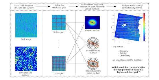
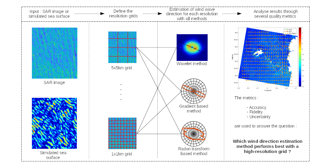
In this article, we focus on three methods to estimate wind direction from a sea surface SAR image in order to evaluate which one offers the best performances and to allow further studies like [12,13,14] to estimate the wind direction and wind speed with the lowest errors and uncertainties. These methods provide a local direction by processing SAR image cells of size around 5 × 5 km. However, in coastal area, the cells have to be finer since the spatial variability is more important than in an offshore area due to bathymetry or wave interaction with coasts. Thus, the aim of this study is to compare the robustness of the methods while the cells dimensions are decreased. In Section 2, we present the two main existing wind direction extraction methods through a State of the Art. A new way to extract the main direction from space wavelet coefficient is proposed in Section 3. Then, we compare the methods accuracy by simulating sea surface in Section 4. Finally, we propose quality metrics as fidelity in Section 5 or the estimation uncertainty in Section 6.

2. State of the Art

In the literature, two main wave direction estimation methods can be found. The first is based on the 2D Fourier Transform [15] and the second on gradient computation [16]. To explain these approaches, we apply them on the SAR image example represented on Figure 1. It may be useful to specify that to enhance the usability of a SAR image in the context of marine remote sensing, several steps, which can be done with the ESA free software ©SNAP, are necessary. The first one is masking land to avoid trying to estimate wind orientations on these areas. The next step is to calibrate the data to make them independant of incidence angle and so get the NRCS values. The third processing is to reduce speckle by choosing an adapted filter as the Lee’s one which uses the local statistical characterizations to smooth homogenous areas and keep the edges information [17]. Finally, the image is projected into the Earth’s coordinates by making a range-Doppler terrain correction. We apply these pre-processing on all SAR images presented in this paper.

The SAR image on Figure 1 is optimal for a clear understanding of the methods since it contains waves with two distinct frequencies and directions. The lowest frequency component corresponds to the gravity waves and the highest frequency to the wind waves [18].

2.1. Wavelet Method

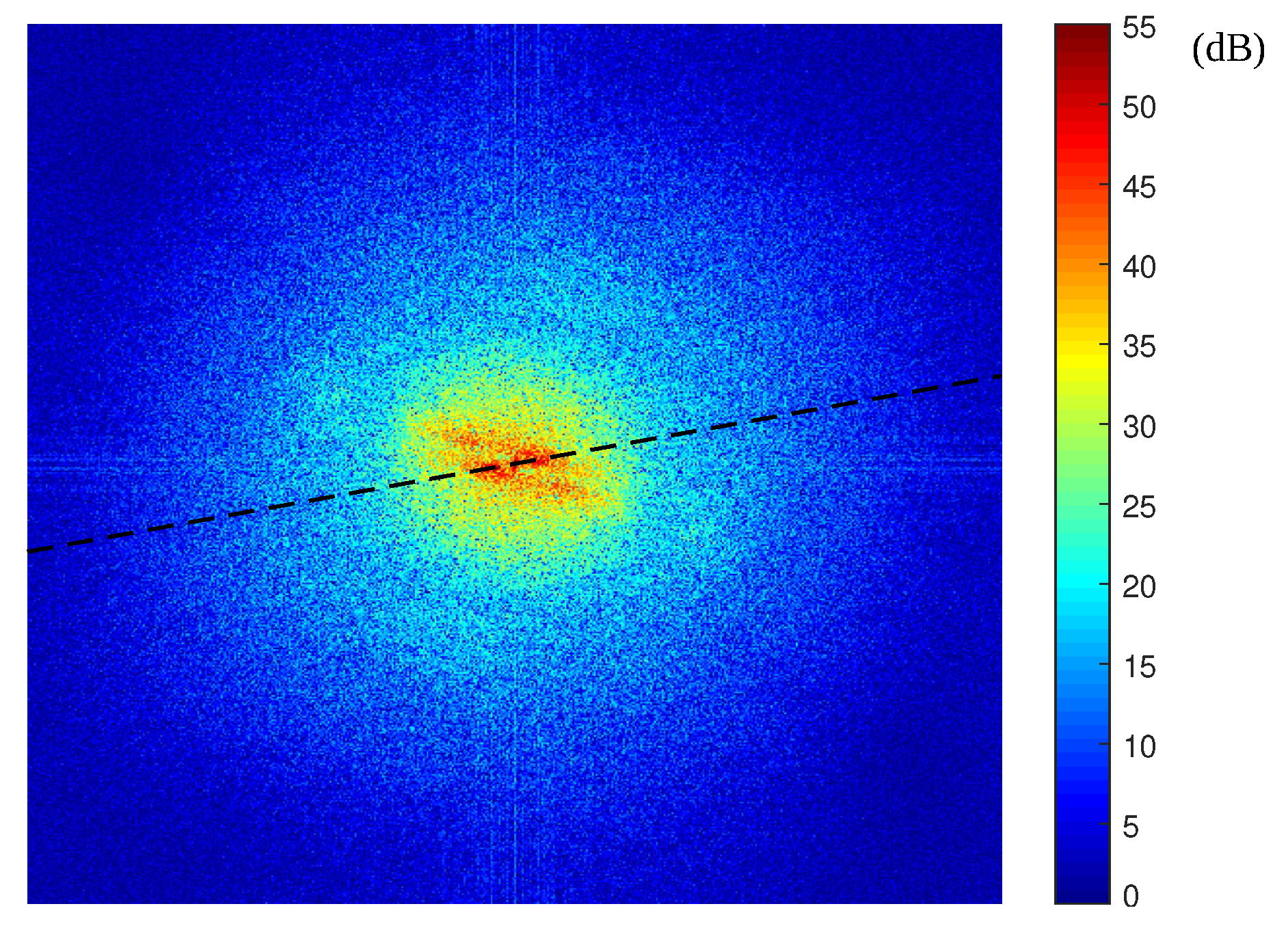
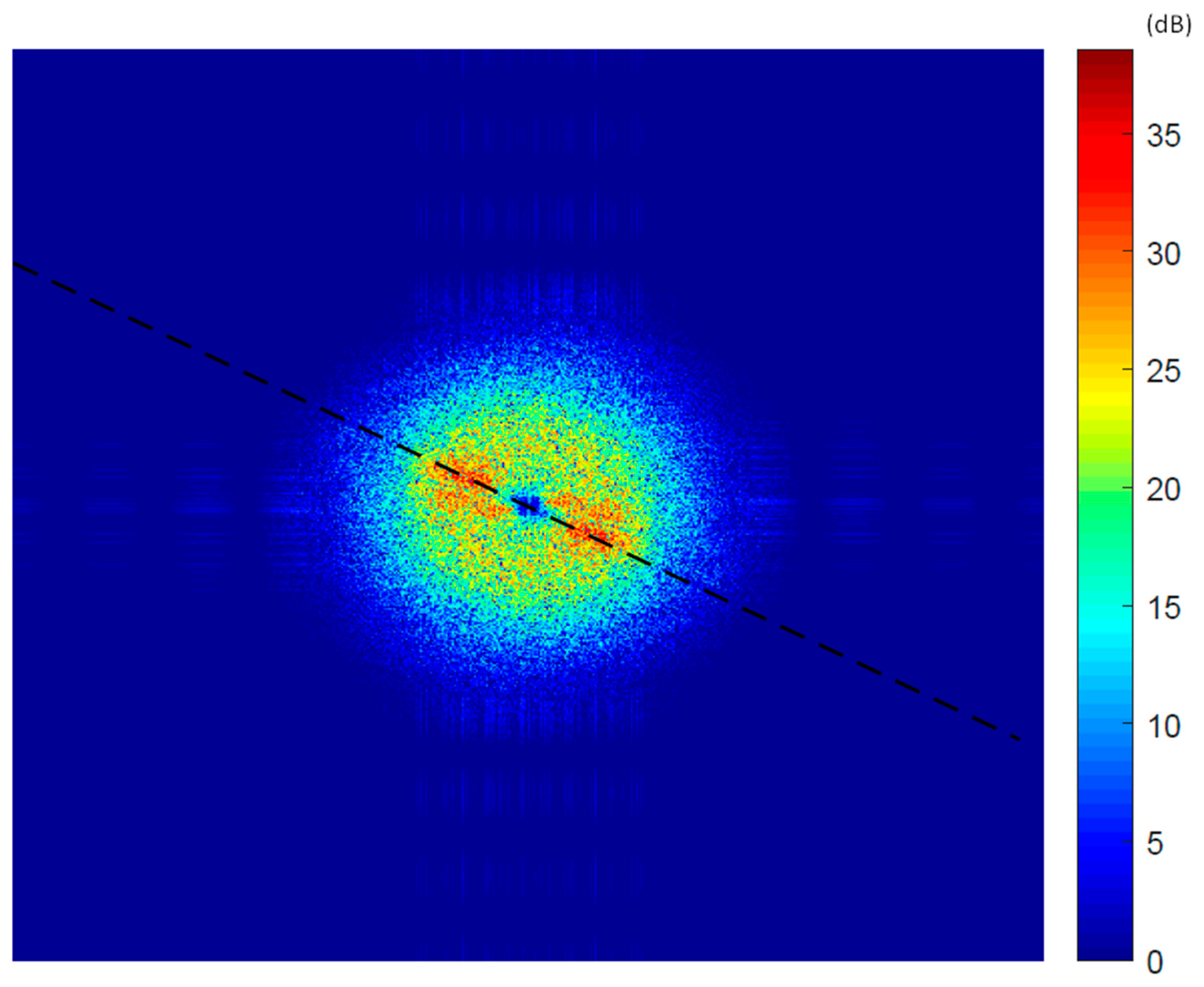
The wavelet method [15] is based on the 2D Fourier transform (2DFT) which shifts the image from the space domain to the frequency-direction domain. The 2DFT of the previous SAR image example is represented on Figure 2. The two frequency components are clearly identifiable by the two pairs of maxima. To automatically find the wave directions, we simply take the orientation of the line that joins the dominant pair of maxima as it can be seen on the same figure. However, in this example, the dominant frequency results from the gravity waves and not from the wind waves.

The spatial wavelet method consists in applying a low-pass filter (LPF) to isolate wind waves wavelength-band in the SAR image I. The result is called the $k^{th}$ wavelet coefficient $C_k$. For $k=1$ we have:

$$C_1=LPF\left\{I\right\}-I$$

(1)

For $k>1$, we take the $k^{th}$ approximation designed by $I_k=\stackrel{ktimes}{\overbrace{LPF\circ LPF\circ \dots \circ LPF}}\left\{I\right\}$, with ∘ the function composition operator, and we have:

$$C_k=I_k-I_{k-1}$$

(2)

The retained level k for the study depends on the SAR image resolution, the low-pass filter parameters and the wavelength band to isolate.

We apply this method on the SAR image with a gaussian filter to isolate the wavelength band 250–500 m and it can be seen on Figure 3 that only the wind waves frequency components are taken into account for the wave direction estimation. The noise frequencies are also cut off.

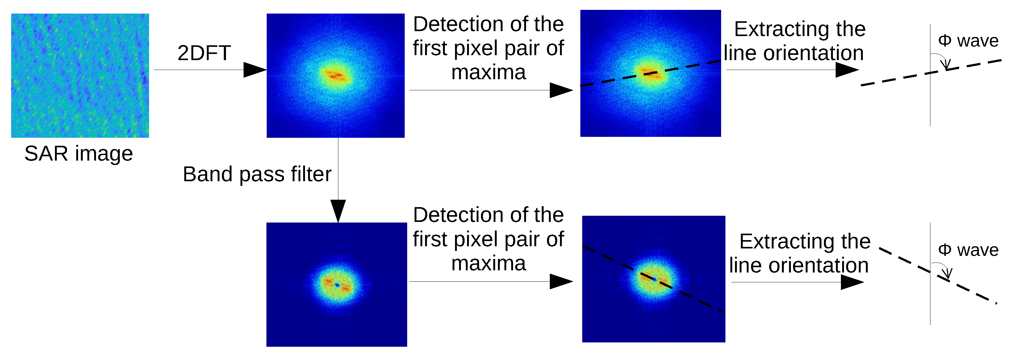
To summarize the 2DFT based methods, we illustrate them on Figure 4. The first line shows the classical method that looks for the orientation ${\mathsf{\Phi }}_{wave}$ of the line that connects the maxima on the raw 2DFT. The second line designates the wavelet method where the orientation of the line is no longer searched on the raw 2DFT but on one of its wavelet coefficient where is isolated the wind wave wavelength.

2.2. Histogram of Oriented Gradient

The Histogram of Oriented Gradient (HOG) is often used in computer vision to recognize gesture [19] but is also applied on SAR images to extract sea wave directions [16]. Its principle is based on the 2D gradient computed thanks to the Optimized Sobel Operator described in Equation (3):

$$D_x=D_y^T=\frac{1}{32}\left[\begin{array}{ccc}3& 0& -3\\ 10& 0& -10\\ 3& 0& -3\end{array}\right]$$

(3)

The gradient horizontal $G_x$ and vertical $G_y$ components of an image I are given by the convolution products:

$$\left\{\begin{array}{c}{G}_x=D_x\ast I\hfill \\ G_y=D_y\ast I\hfill \end{array}\right.$$

(4)

Then, the gradient amplitude A and the gradient orientation $\mathsf{\Phi }$ are:

$$\left\{\begin{array}{c}A=\sqrt{G_x^2+G_y^2}\hfill \\ \mathsf{\Phi }={tan}^{-1}\left(\frac{G_y}{G_x}\right)\hfill \end{array}\right.$$

(5)

Finally, the HOG is the histogram (to visualize the histograms more clearly, we plot them in a polar coordinate system. From now on and for the rest of the article, we take as convention $0^{°}$ corresponding to the north, ${90}^{°}$ to the east, ${180}^{°}$ to the south and ${270}^{°}$ to the west.) of the matrix $\mathsf{\Phi }$ weighted by the corresponding value of the matrix A [19]. 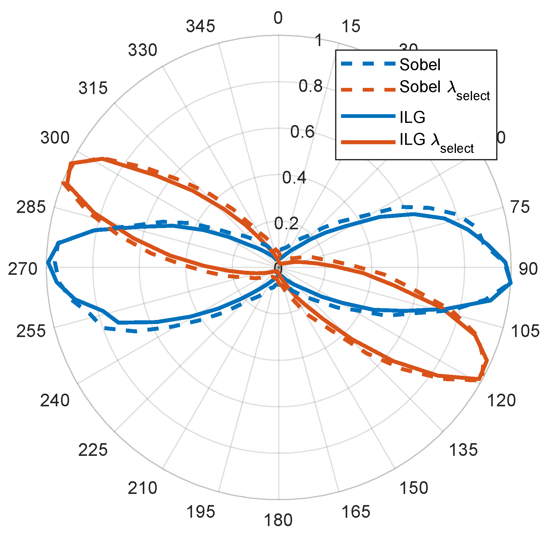The result is given on Figure 5 by the dotted blue line. The direction is given by the histogram maxima. We can also apply the HOG method on the wavelet coefficient corresponding on the wind wave wavelengths, which gives the orange dotted histogram that indicates the wind waves direction.

The gradient computation can be enhanced with an improved local gradient (ILG) [20]. The ILG is no more than the Hadamard product of the SAR image and the gradient amplitude A computed with the Sobel optimized operator. The full blue and orange curves on Figure 5 show the HOG computed with the ILG method, respectively with and without bandpass filter. In the two cases, the histogram lobe is thinner, implying a reduction of the estimation uncertainty.

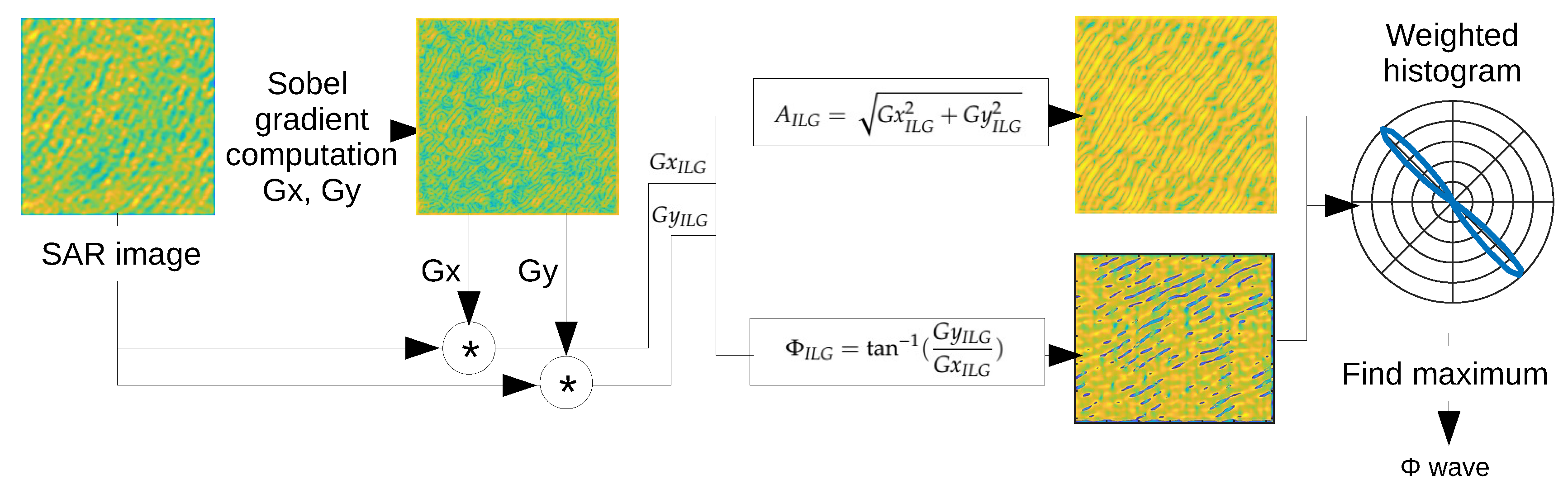
The different steps of the gradient based method are illustrated in Figure 6. The SAR image gradient horizontal and vertical components $G_x$ and $G_y$ are computed with the Sobel operator. Then, these components are convolved with the SAR image, which gives the ILG components $G{x}_{ILG}$ and $G{y}_{ILG}$. These quantities are then used to compute the gradient amplitude $A_{ILG}$ and orientation ${\mathsf{\Phi }}_{ILG}$ which are employed to compute the histogram of ${\mathsf{\Phi }}_{ILG}$ weighted by $A_{ILG}$. Finally, the sea wave direction ${\mathsf{\Phi }}_{wave}$ is estimated as the angle where the maximum of the histogram is reached.

It worth notice that all the methods presented provide the wave direction with an ambiguity of ${180}^{°}$. To remove this ambiguity, we can use wind shadow [21] or Doppler information [22].

3. Extracting Wavelet 2DFT Main Direction with the Radon Transform

We propose to apply the Radon transform, a classic mathematics tool used in tomography [23], on the 2DFT to detect the dominant direction. The pixels $I_{FT}(i,j)$ of the 2DFT $I_{FT}$ are projected on a line $\xi$ oriented by an angle $\theta$. This projection is described in Equation (6):

$$RT(\xi ,\theta )=\sum _i\sum _j{I}_{FT}(i,j)\delta (icos\left(\theta \right)+jsin\left(\theta \right)-\xi )\mathsf{\Delta }i\mathsf{\Delta }j$$

(6)

With $\delta$ the Dirac function and $\mathsf{\Delta }i=\mathsf{\Delta }j=1$ the pixel steps. What we need is simply the projection on the center for all angles $\theta$ i.e., $RT(\xi =0,\theta )$.

To avoid the projection of residual noise frequencies or sinc pattern due to FT computation, the 2DFT can be thresholded by an adaptated method as the Otsu threshold [24]. Its principle is to binarize a gray-scale image by getting the statistical properties of the image histogram to minimize the pixels intra-class standard deviation. This method can be generalized as a multi-Otsu method to allow segmentation for a N classes problem. Thus, to mask the 2DFT undesired low values without altering useful information, we apply the multi-Otsu method for a 2 classes problem.

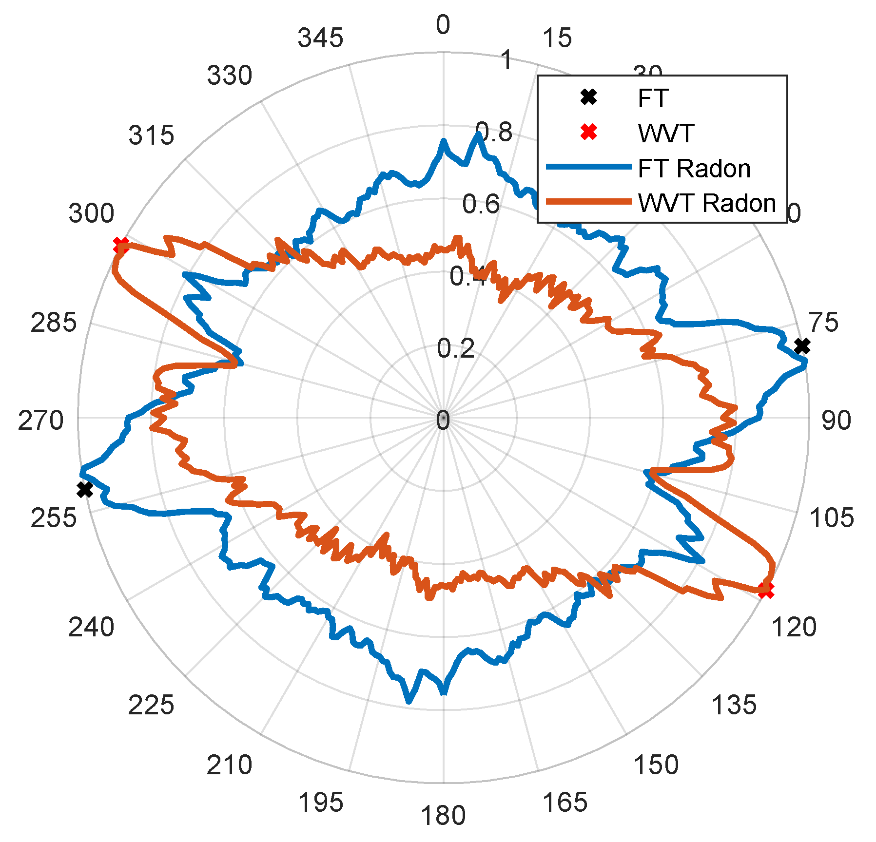
Finally, the masked 2DFT projection normalized by its maximum is represented in the polar coordinate system on Figure 7. The blue and orange lines correspond respectively to the projection of Figure 2 and Figure 3 and the black and red crosses are waves directions estimated by linking the dominant pair of 2DFT maxima.

The Radon angles where the projection maximum are reached are in adequacy with the black and red crosses. Thus, the Radon projection can be used to estimate the waves direction and we define this estimated direction in Equation (7):

$${\mathsf{\Phi }}_{wave}=\underset{\theta }{\mathrm{argmax}}RT(\xi =0,\theta )$$

(7)

4. Assessment of Direction Estimation Method Accuracy with Simulated Sea Surface

4.1. Sea Surface Simulation

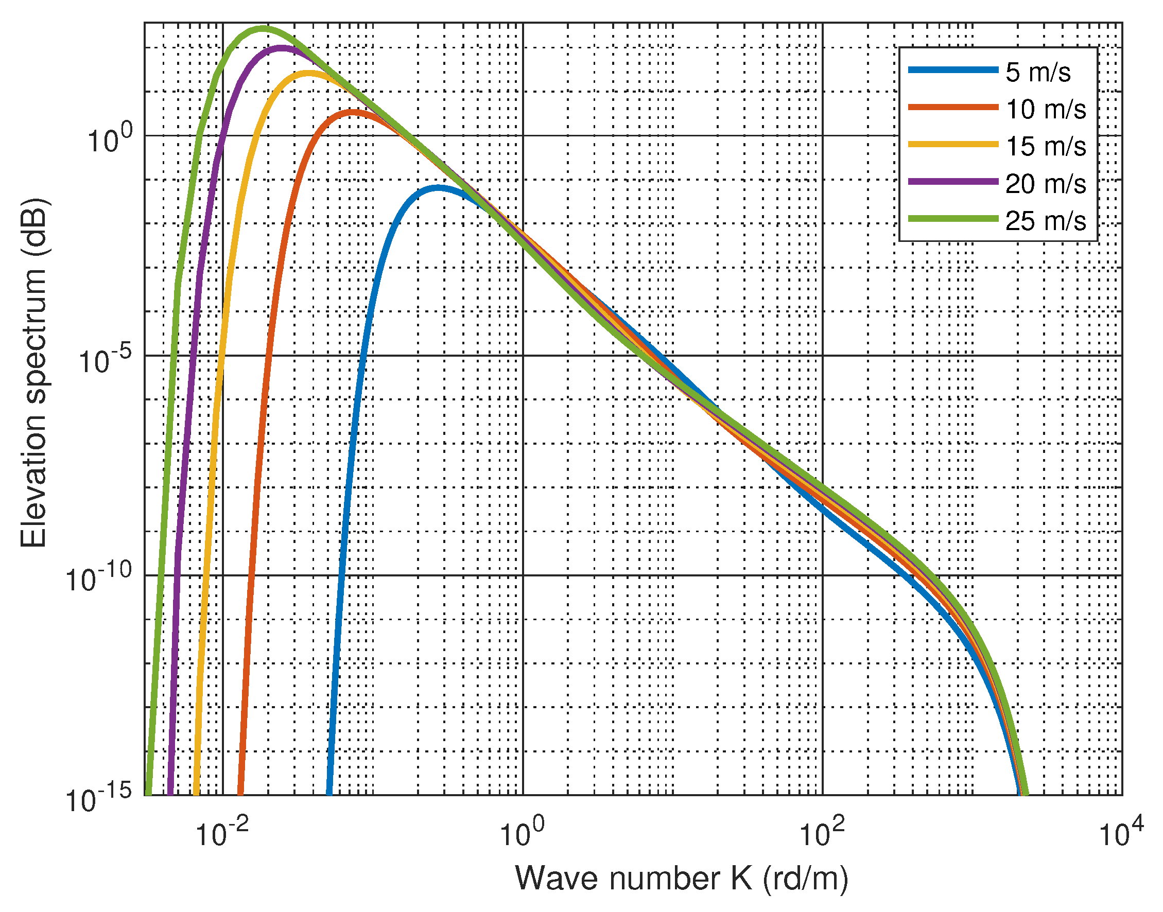
In this section, we apply the wind direction extraction methods on simulated sea surfaces. To simulate this type of surface, we choose a spectral approach. Several models of roughness spectra exist but the Elfouhaily spectrum [25] is the only one in adequacy with the in situ measurements of Cox and Munk [26]. Moreover, it allows to take into account the fetch, which is useful in the context of a coastal environment where the sea is not fully developed. The Elfouhaily monodirectional spectrum S(K) in function of the wave number $K=\frac{2\pi }{\lambda }$ is presented on Figure 8. We observe the contribution of gravity waves increasing with wind speed while the capillary waves contribution variation is less influential.

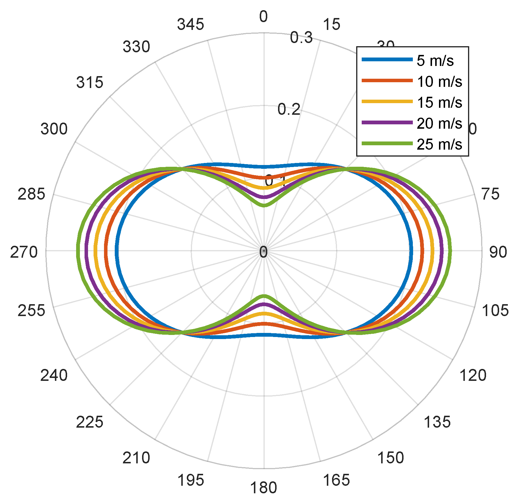
Then, to take the wind direction into account, an angular repartition function by Elfouhaily [25] and is described by the following expression:

$$f(K,\mathsf{\Phi })=\frac{1}{2\pi }[1+\mathsf{\Delta }\left(K\right)cos\left(2\mathsf{\Phi }\right)]$$

(8)

with $\mathsf{\Phi }$ the angle between the wind direction and the propagation direction of the K wave number component. The information provided by this function is interesting. As we can see on Figure 9, a high wind speed induces more finely directed waves than a low wind speed. This behaviour is consistent since the gravity waves tends to have a unique direction while the capillary waves are distributed for more angles.

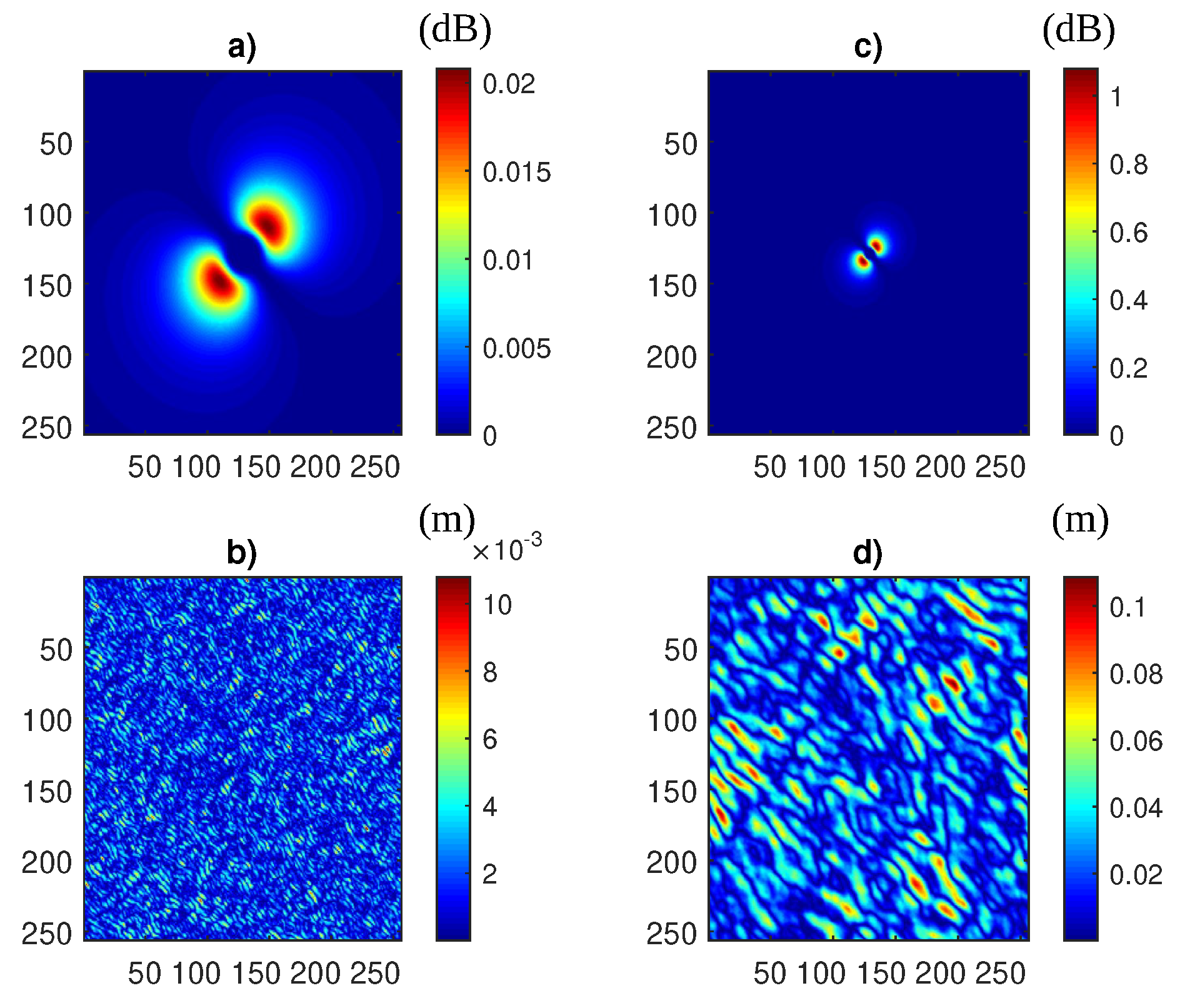
The complete Elfouhaily spectrum is the product of the monodirectional spectrum and the angular repartition function:

$$S(K,\mathsf{\Phi })=S\left(K\right)f(K,\mathsf{\Phi })$$

(9)

This spectrum is represented on Figure 10a,c respectively for wind speeds of 5 m/s and 10 m/s. To compute the surface associated, a gaussian noise is filtered by the spectrum. The results are given on Figure 10b,d where the sea wave frequency is higher for low wind speed and the elevation is higher for high wind speed.

4.2. Results and Discussion

In this section and in the following ones, we compare three wave direction estimation methods that we abbreviate as:

• HOG for the Histogram of Oriented Gradient computed with the Improved Local Gradient,
• WVT for the wavelet method with the extraction on the 2DFT by linking the dominant pair of maxima,
• WVT Radon for the wavelet method with the extraction on the 2DFT masked with Otsu by taking the maximum of the Radon projection.

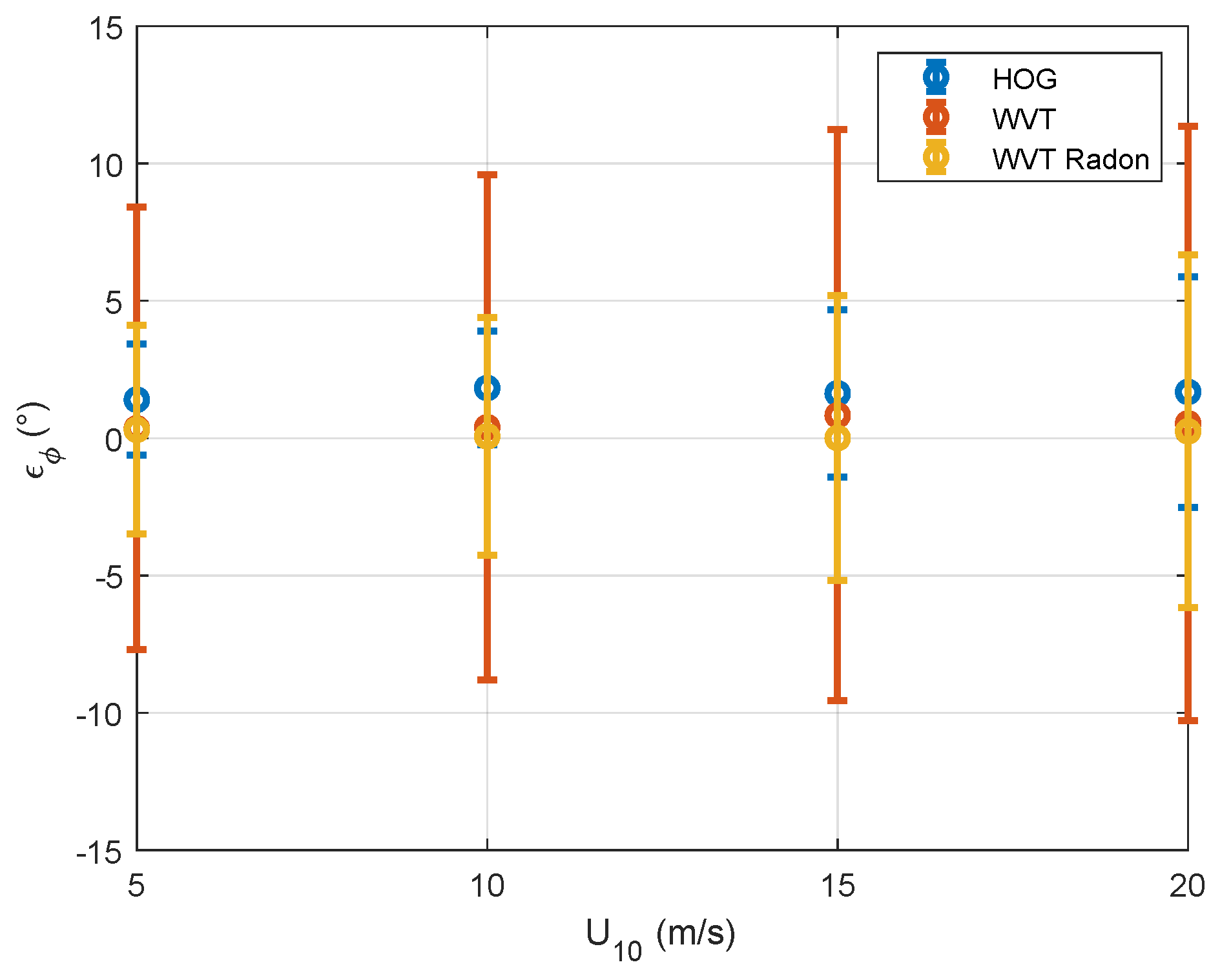
These three algorithms are applied on simulated sea surfaces with wind speeds from 5 to 20 m/s with a step of 5 m/s. For each wind speed, we simulate 500 surfaces to compute significant statistical quantities of the direction estimation error ${ϵ}_{\mathsf{\Phi }}$. The error mean and standard deviation are presented in function of wind speed on Figure 11.

First of all, by observing the general behavior of the methods estimation error, we notice that for all wind speeds their averages are close to $0^{°}$ and their standard deviations vary little. These standard deviations range from 5 to 12${}^{°}$, which does not seem excessive since the accuracies found in the literature range from 15 to 40${}^{°}$ [27].

Second, all three methods have a standard deviation that increases with wind speed and therefore give less reliable results for strong winds. This observation does not seem logical when considering the angular distribution function: the direction should be easier to estimate with high wind speed because gravity waves have a more marked direction (see Figure 9). However, as we have seen on the Elfouhaily spectrum, the stronger the wind, the more dominant the low frequencies are. Thus, the amount of data in the wind wave wavelength band retained by the wavelet filter is lower as the wind speed increases. Thus, we have less information to estimate the desired direction, which justifies the higher probability of error.

We now compare the methods with each other. First, we notice that the Radon projection reduces the standard deviation of the WVT method. This can be explained by the inclusion of more information in the 2DFT by the WVT Radon method. Indeed, the bandpass filter is not perfect, so there may be some undesirable residuals that may falsify the results of the WVT method. Secondly, the WVT Radon method has the best accuracy for all wind speeds since its average error is the lowest. Finally, the HOG method has the lowest standard deviation error for all wind speeds and is therefore the most reliable method.

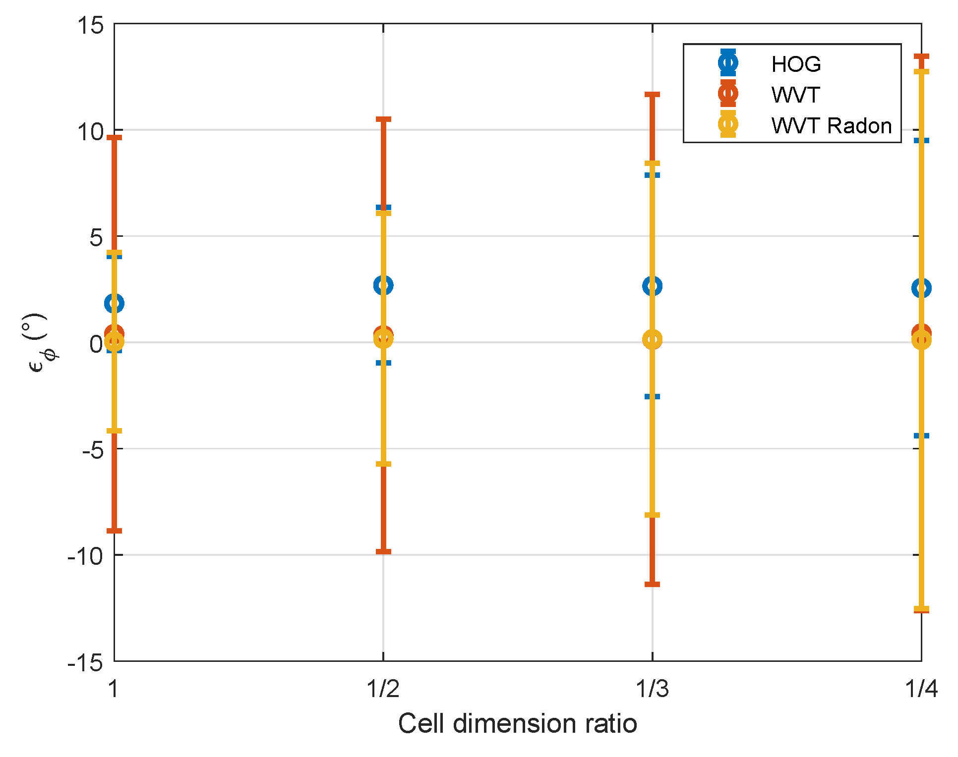
In a second time, we study the behavior of the methods when the dimensions of the local area are decreased by taking sub-images on simulated sea surfaces. These cell dimensions are $\frac{1}{2}$, $\frac{1}{3}$ and $\frac{1}{4}$ times the original dimensions. The results are given on Figure 12 where the error is represented in function of these dimension ratios. First of all, the reliability of the methods declines with the reduction of dimensions, which is logical since the amount of information decreases.

Then, it can be pointed out that the WVT and WVT Radon methods are more accurate for all the dimensions of the cell. However, they are more sensitive to dimension reduction because their error standard deviations are twice as high as the HOG one for the smallest cell. The HOG method appears to be more reliable for a high-resolution grid.

Finally, by comparing Figure 11 with Figure 12, we can assume that the dependence of the error on wind speed, for speeds between 5 and 20 m/s, is negligible compared to the effects of cell dimensions. Indeed, the error standard deviation varies little with the wind speed and almost triples as a function of the cell dimensions. Thus, the influence of cell dimensions can be studied independently of wind speed.

5. Assessment of Direction Estimation Method Fidelity with RADARSAT-2 Data

5.1. RADARSAT-2 Data

In this section, we work on a RADARSAT-2 product taken towards the Ouessant Island and Molene archipelago on 29 December 2019 with a resolution of 6.5 m. We apply the three methods on this SAR image with cell dimensions of 2 × 2 km and the results are shown on Figure 13.

5.2. Quality Metric

It is difficult to assess the accuracy since wind in situ data from buoys, ships or weather stations are limited. So, we focus on the methods fidelity: a quality indicator that can be compared to the error ${ϵ}_{\mathsf{\Phi }}$ variance saw in the simulation part. To get access to this quantity, we have to estimate wave direction on several regions of an homogeneous sea area.

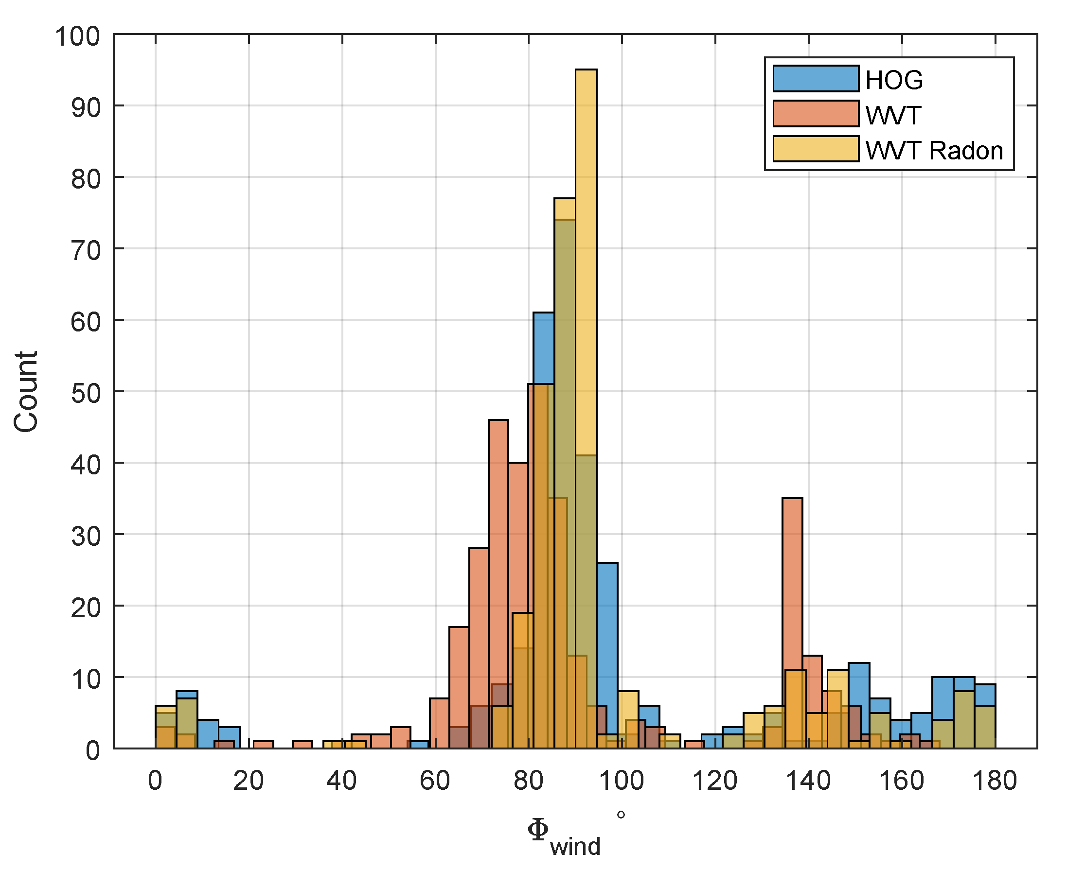
As it can be seen on Figure 13, there are two main area, delimited by the red border, where the estimated wave directions are almost constant. To highlight the presence of these two area, the histogram of estimated directions is represented on Figure 14. The area can be divided into a class $C_1$ containing estimated wind directions from west to east (i.e., angles of ${90}^{°}\pm {30}^{°}$) and another class $C_2$ for directions from northwest to southeast (i.e., angles of ${150}^{°}\pm {30}^{°}$). The class $C_1$ can be considered as an offshore area and the class $C_2$ is an ocean part protected by the archipelago from the open sea waves.

5.3. Results and Discussion

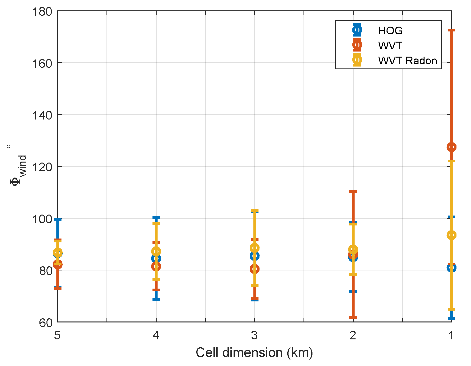
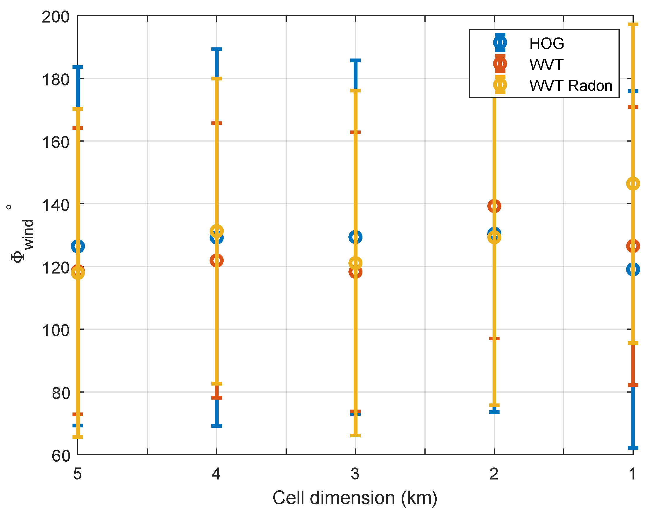
We apply the methods on cells belonging to classes $C_1$ and $C_2$ separately by reducing their dimensions. To select a class, we choose to take the union of the three methods estimations belonging to the desired class. For the class $C_1$, the direction estimations mean and standard deviation are given in function of the cell dimensions on Figure 15.

First, the general behavior is logical because the larger the cell dimensions, the more reliable the methods are, i.e., The smaller the standard deviation of the estimates; and consistent, i.e., The means are approximately constant with respect to the cell dimensions, except for the dimensions of 1 km × 1 km.

Then, we retrieve the observations of the simulation part: the Radon projection inclusion in the WVT method induces a gain in fidelity because the standard deviation of WVT Radon estimations is lower than the WVT method ones. Moreover, for 1 km cells, the WVT Radon method has a better coherency than the WVT method since this last method estimations mean does not match with results for other cell dimensions. However, the incoherence of the WVT method calls into question its accuracy for small cells obtained in the simulation part.

Finally, the HOG method provides almost constant estimates regardless of cell size and has the best performance (fidelity and consistency) for small cells. These comments reinforce those reported in the simulation section.

Now, we focus on the class $C_2$. The results on Figure 16 are not as easy to exploit as the previous ones since it represents estimations on a sea surface disturbed by bathymetry and coasts. Moreover, it can be seen on Figure 13 that the angles in the range 30${}^{°}$ ± 30${}^{°}$ are part of coastal area and corresponds to the estimation errors. Moreover, the area selection is not perfect. That can justify the high standard deviation, which is so important that we cannot make any conclusion in that case.

6. Assessment of Direction Estimation Method Uncertainty with Sentinel-1 Data

6.1. Sentinel-1 Data

In this section, we work on some offshore SAR images from Sentinel-1. We take 20 SAR images from the European Space Agency (ESA) database (https://scihub.copernicus.eu) and we extract 10 subimages of 5 × 5 km from each of them. So, we study 200 SAR samples from different date and under different weather conditions with a resolution of 12.5 m.

6.2. Quality Metric

We define the dynamic D of a function f in Equation (10) as the distance between the function maximum and its other values.

$$D=\frac{1}{N}\sum _{i=1}^N(max\left\{f\left(x_i\right)\right\}-f\left(x_i\right))$$

(10)

This quantity provides information on how a peak is distinguishable from its neighbouring values. Thus, if the dynamic tends towards 1, the function f tends to a Dirac function and there is no ambiguity to find the maximum position. On the contrary, if it is near to 0, the function is almost constant and there is a high uncertainty for the maximum position. So the higher dynamic, the lower uncertainty.

6.3. Results and Discussion

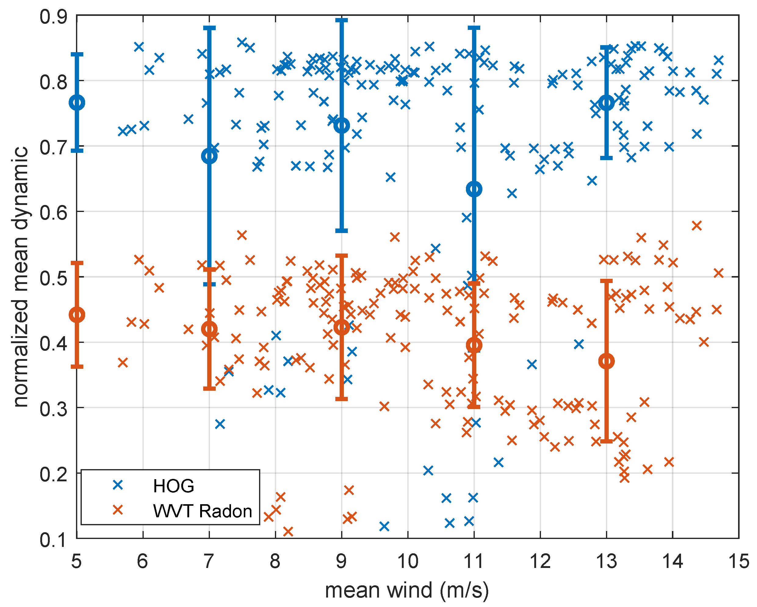
As the dynamic cannot be computed for the WVT method, we only compare the HOG and WVT Radon normalized dynamics. We begin to study this metric in function of wind speed on Figure 17. To estimate the wind speed on a cell, we apply the CMOD5N model [7] on the NRCS values and we retain the mean wind speed.

Necessarily, for all wind speed, HOG has better dynamic since the WVT Radon projects undesired values, what we could have predicted by looking at Figure 5 and Figure 7. But what is interesting to see is that the influence of wind speed on dynamic is negligible because the metric mean for both methods are almost constants according to the wind speed. Thus, the earlier hypothesis of wind speed independency is reinforced, for wind speeds between 5 and 15 m/s.

Finally, we study the dynamic for the 200 SAR samples in function of cell dimensions on Figure 18. The dynamic decreases as expected with the dimensions, so the uncertainty is higher for small cells. It can also be seen that for all dimensions, the HOG dynamic remains greater than the WVT Radon one. Thus, the HOG estimations have less uncertainty for all cell dimensions.

7. Conclusions

The aim of this study is to evaluate the performance of different wave direction estimation methods on SAR images. We focus specifically on their behavior when we search to refine the spatial resolution of the estimation grid.

We propose to enhance the wavelet method thanks to the Radon transform and we compare this improvement with classical methods such as HOG or wavelet through different quality metrics depending on the spatial resolution of the estimations.

The first metric is the accuracy obtained from simulated sea surfaces. We first notice that the implementation of Radon projection in the wavelet method improves the results by reducing the error standard deviation. Secondly, the wavelet method with Radon has mean errors closest to 0, while HOG has the smallest standard deviations of errors. Thus, the WTV Radon method is the most accurate and the HOG method is more stable for simulated sea surfaces.

In a second time, we introduce new metrics to have information on the estimation quality from real SAR images: the fidelity, related to the estimation standard deviation, and the dynamic, representing the uncertainty for an estimate. For the fidelity, we work in a homogeneous area and we find that the HOG method has the best fidelity when we work on cells with dimensions from 5 km to 1 km. We also observe that for these dimensions, the Radon projection greatly improves the fidelity of the wavelet method. For the dynamic, we observe that the HOG method presents less uncertainties than the wavelet method improved with the Radon projection.

Using these indicators, we conclude that the HOG method has better fidelity and lower uncertainty than wavelet methods for small cells in an offshore area. However, wavelet methods seem to have a better accuracy through simulation study but this observation is questioned by the coherence analysis on the RADARSAT-2 image.

8. Perspectives

The results given for the accuracy in the simulation part are not entirely valid. Indeed, we only simulate a sea surface and not a SAR image where visible sea waves depends on the interaction of electromagnetic wave and the sea surface: the NRCS is maximal when the electromagnetic waves frequency is approximately equal to the sea waves frequency. This phenomenon is called the Bragg resonance [18,28]. Thus, the SAR image does not represent all the sea surface details and it would be a further work to simulate SAR images with a low calculus time to assess the wind direction extraction methods accuracy.

Moreover, we manage to compare the methods in offshore area images. The cases of coastal area is more complexe and would deserve to be further studied. We tried to weight the estimations with the dynamic to have more significant statistical information than those on Figure 16 but the results were not easier to exploit. A solution would be to enhance the area classification e.g., with a deep learning algorithm.