Abstract
Object detection and recognition in aerial and remote sensing images has become a hot topic in the field of computer vision in recent years. As these images are usually taken from a bird’s-eye view, the targets often have different shapes and are densely arranged. Therefore, using an oriented bounding box to mark the target is a mainstream choice. However, this general method is designed based on horizontal box annotation, while the improved method for detecting an oriented bounding box has a high computational complexity. In this paper, we propose a method called ellipse field network (EFN) to organically integrate semantic segmentation and object detection. It predicts the probability distribution of the target and obtains accurate oriented bounding boxes through a post-processing step. We tested our method on the HRSC2016 and DOTA data sets, achieving mAP values of 0.863 and 0.701, respectively. At the same time, we also tested the performance of EFN on natural images and obtained a mAP of 84.7 in the VOC2012 data set. These extensive experiments demonstrate that EFN can achieve state-of-the-art results in aerial image tests and can obtain a good score when considering natural images.
1. Introduction
Remote sensing imaging techniques have opened doors for people to understand the earth better. In recent years, as the resolution of remote sensing images has increased, remote sensing target detection (e.g., the detection of aeroplanes, ships, oil-pots, and so on) has become a research hotspot [1,2,3,4,5]. Remote sensing target detection has a broad range of applications, such as military investigation, disaster rescue, and urban traffic management. Differing from natural images taken from low-altitude perspectives, aerial images are taken from a bird’s-eye view, which implies that the objects in aerial images are arbitrarily oriented. Moreover, in many circumstances, the background is complex and the targets are densely arranged, often varying in shape and orientation. These problems make target detection using aerial images very challenging. Most advanced object detection methods rely on rectangular-shaped horizontal/vertical bounding boxes drawn on the object to accurately locate its position. In the most common cases, this approach works; however, when it comes to aerial images, its use is limited, as shown in Figure 1a. Such orthogonal bounding boxes ignore the object pose and shape, resulting in reduced object localization and limiting downstream tasks (e.g., object understanding and tracking). In this case, an oriented bounding box is needed to mark the image area more accurately, as shown in Figure 1b.
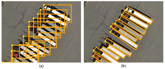
Figure 1.
A group of large vehicles with different annotation methods: (a) shows a failure case of horizontal rectangle annotation, which leads to high overlap, compared to (b).
Benefitting from R-CNN frameworks [2,4,6,7,8,9,10,11], many recent works on object detection in aerial images have reported promising detection performances. They have used the region proposal network (RPN) to generate regions of interest (RoIs) from horizontal bounding boxes, followed by identifying their category through region-based features. However, [5,12] showed that these horizontal RoIs (HRoIs) typically lead to misalignments between the bounding boxes and objects. As a result, it is usually difficult to train a detector to extract object features and identify the object’s localization accurately. Instead of using horizontal bounding boxes, many methods regress the oriented bounding boxes by using rotated RoIs (RRoIs). In [5,12,13,14,15], rotated anchors are added on the basis of the original. In order to achieve a higher recall rate in the regional proposal stage, they use anchors with different angles, scales, and aspect ratios. The rapid increase in the number of anchors makes the algorithm very time-consuming, however. [16,17] designed a converter to transform HRoIs into RRoIs. Although this method reduces the time consumption due to anchors, it also has a more complex network structure.
FCN [18] brought semantic segmentation into the deep learning era, being the first pixels-to-pixels semantic segmentation method which was end-to-end trained. Compared with patch-wise classification for object detection, semantic segmentation can better carry out spatial context modeling and avoid redundant computation on overlapping areas between patches. Many applications using semantic segmentation techniques have been proposed in the remote sensing literature, such as building extraction [19,20,21,22], road extraction [23,24,25,26,27], vehicle detection [28], land-use and land-cover (LULC) classification [29,30,31], and so on. The main methodologies in these works follow general semantic segmentation but, for some special application scenarios (e.g., vehicles or buildings), many improved techniques [20,25,27] have been proposed for the application scenario. However, semantic segmentation requires pixel-wise annotation, which greatly increases the cost of data annotation. At the same time, due to its inability to distinguish intra-class instances, it is not suitable for scenes with densely arranged targets.
We start with the structure of the network. Features encoded in the deeper layers of a CNN are beneficial for category recognition, but not conducive to localizing objects. The pooling layers in a CNN preserve strength information and broaden the receptive field, while losing location information to a great extent. Relative works [9,32,33,34] have shown that the descriptors have a feeble ability to locate the objects, relative to the center of the filter. On the other hand, many related works [35,36,37] have shown that learning with segmentation can lead to great results. Edges and boundaries are the essential elements that constitute human visual cognition [38,39]. As the feature of semantic segmentation tasks captures the boundary of an object well, segmentation may be helpful for category recognition. Secondly, the ground-truth bounding box of an object is determined by its (well-defined) boundary. For some objects with non-rectangular shapes (e.g., a slender ship), it is challenging to predict high IoU locations. As object boundaries can be well-encoded in semantic segmentation features, learning with segmentation can be helpful in achieving accurate object localization.
To this end, we propose the ellipse field network (EFN), a detector with a more efficient network structure and a training method that preserves location information. EFN can be regarded as the supplement and upgrade of general semantic segmentation, which has a strong ability for pixel-by-pixel classification and can achieve fine-grained region division. The main problem is that pixels of the same kind are connected, while the sort of each pixel is isolated, such that we cannot obtain the comprehensive information of an object, nor the number of objects, which is difficult to carry out without adequate semantic understanding. EFN proposes the concept of an object field (OF), which is defined as a probability density function describing the distribution of objects in image space; it is composed of a center field (CF) and an edge field (EF). Luo et al. [40] showed that an effective receptive field follows a Gaussian distribution. In combination with practical results, we consider that the 2D Gaussian distribution is an appropriate choice for the object field [41]. The intensity distribution of the Gaussian distribution is related to the elliptic equation (as shown in Figure 2b), which is why we call this method the ellipse field network. Besides, we designed a special post-processing step for the object field—ellipse region fitting (ERF)—which combines the center field and the edge field, in order to finally obtain the ellipse region set of objects. In summary, our work provides several advantages:
- The unique field-based framework design, combined with the feature map concatenation operation, enables the network to learn features and location information better.
- It combines the advantages of object detection and semantic segmentation and, so, can finely locate and classify each instance.
- Ellipse region fitting: the corresponding post-processing process makes the results more robust and reliable.
- An effective image mosaic method called spray painting is proposed, in order to process high-resolution images.
The rest of the paper is organized as follows: After the introductory Section 1, detailing object detection in aerial images, we enter Section 2, which is dedicated to the details of the proposed EFN. Section 3 then introduces the spray painting and post-processing step we designed for EFN, while Section 4 provides data set information, implementation details, experimental results, and discussion. Finally, Section 5 concludes the paper.

Figure 2.
Overall pipeline: (a) input; (b) Center Field (top) and Edge Field (bottom); (c) post-processing by ellipse region fitting (ERF); and (d) the detection result.
2. Ellipse Field Network
Figure 3 illustrates our network architecture. EFN is orthogonal to special network design and, so, any FCN backbone architecture can adapt to it. Here, we use U-net [42] as an example. EFN takes images with proper resolution as input and processes them through several convolutional, max pool, and concatenate layers. Then, the output is branched into two sibling output layers: one is the object field, while the other is the edge field. Each output layer has several channels corresponding to the number of categories. After that, the ERF algorithm processes the output to obtain the center and edge points of each object and finally outputs an ellipse. As shown in Equation (1), we use five parameters: , , a, b, and to define an ellipse, where are the co-ordinates of the center point of the ellipse, are the semi-major axis and the semi-minor axis, respectively, and is the angle of rotation. The function describes the relationship between a point and an ellipse.
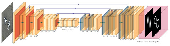
Figure 3.
Visualization of the network architecture. In the input image, the target to be detected is two airplanes. The output of the network is two fields describing the distribution probability of the center and edge of the target. The input passes through some convolutional and pooling layers to extract features. Then, through several concatenations, convolutions, and bilinear interpolations, the output results are obtained.
2.1. Center Field
The center field represents the distribution of intensity, which describes the distance between the pixels and center point of objects. According to Equation (1), if a pixel is inside an object or on its edge, . Based on this, we define , the center field intensity of a pixel, in Equation (2). In the equation, is a coefficient which we call the center field decay index (with default value of 2.5), which determines the decay rate. When objects are densely packed, some points may belong to more than one ellipse; in this case, we choose the ellipse which has minimum distance to the point. One pixel corresponds to one target, which solves the problem that semantic segmentation can not distinguish intra-class instances. The intensity decays from 1 at the center of an object to at the edge, with a specific rate. In areas containing no objects, the intensity is 0. Figure 4a shows an intensity distribution.
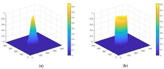
Figure 4.
(a) Visualization of center intensity in image space; and (b) visualization of edge intensity in image space.
2.2. Edge Field
Similarly, the edge field represents the distribution of edge intensity, which describes the distance between pixels and the edges of objects. According to Equation (1), the sufficient and necessary condition of a pixel being on an edge is . Based on this, we define the center field intensity of a pixel in Equation (3). Theoretically, the edge of an object is an elliptic boundary formed by a sequence of connected pixels. In other words, the edge is very slim, which makes it difficult to recognize. To reduce the impact of this, we define a parameter, , called the edge width, in order to adjust the width of the edges. We set the default value as 0.1. Visualization of an edge field is shown in Figure 4b.
2.3. Training Process
When calculating the loss function, the influence of targets with different sizes should be similar. As there are more pixels in a large object and less in a small one, the calculation of loss by pixel accumulation should give a higher weight to the small target. We obtain the area of the rectangle to which the pixel belongs and, then, set the weight according to the reciprocal of the area size, as in Equation (4), where is a bias and the default setting is 0.1:
Finally, the output layer scans the whole output array to determine the distance between each pixel and each ellipse. Then, we obtain the loss, as given in Equation (5), where p represents the pixel of the images, and are the center intensity and edge intensity predicted by the network, respectively, and and are the respective ground truths. In this way, the impact of object size can be reduced, to some extent.
3. Post-Processing
3.1. Spray Painting
Limited by the storage capacity, the input images should not be too large. Thus, high-resolution aerial photos must be cropped into pieces. There may be a large number of objects split at the intersection, which can lead to the errors in the image mosaic. To this end, we propose a novel method which takes advantage of the fields detailed above. The process of common large size image detection methods can be described as , which divides the large image into small images, detects the targets in the small images, uses NMS [43] to remove the redundant bounding box, splices the small image into the large image, and uses NMS again to remove the redundant bounding box caused by splicing. This process has high computational complexity and incomplete objects may be missing or repeat in the margin of patches. The process of our method can be described as , which we call spray painting. Figure 5 demonstrates this process. Concretely, we first generate blocks with overlapped edges, set to 0.2 times the width of the large image by default. Each junction may be composed of 2–4 cropped images; we use a linear weighted algorithm, given in Equation (6), to fuse them. This can lead to a near-seamless large image. In this way, the overhead of image cropping and mosaicking can be greatly reduced. Even on some devices with insufficient computing power (e.g., embedded NPU devices), EFN can process large size images conveniently.
where is the field intensity value and is the shortest distance from the edge of the point mapped to the cropped image at of the large image.
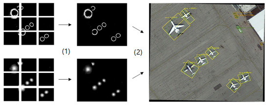
Figure 5.
Spray painting can splice small field images into large ones and, then, obtain a bounding box through ERF.
3.2. Ellipse Region Fitting
The ERF algorithm attempts to figure out the parameters of all ellipses according to the center field and edge field, describing the output information of the network in a mathematical manner to obtain oriented bounding boxes (see Figure 2d; it is the minimum enclosing rectangle of the ellipse). There are three main steps in this algorithm: acquiring the initial center points, acquiring points on the edges, and figuring out reliable parameters.
The first step is to acquire the initial co-ordinates of the center points, according to the center field (which represents the object intensity distribution). For each channel, we scan the elements sequentially. As shown in Figure 6a, if the intensity is , we search for the maximum intensity in the eight pixels around the current one. If the maximum intensity is greater than , we keep searching from the new pixel until there is no pixel greater and record its co-ordinates . After processing a channel, we obtain a group of local maximum co-ordinates of pixels, which are the initial co-ordinates of the center points of a category object.
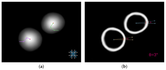
Figure 6.
Solution procedure: (a) Approximately demonstrate the way to find the center point of fields; (b) two points found by our method, which the rest can be deduced from.
The second step is to acquire the points on the edges. The edge field represents the edge intensity distribution. We start from the initial center points acquired from the first step, producing a beam every three degrees from 0° to 360°. As shown in Figure 6b, along with the beam, jumps somewhere and decays away from the center point. If the of a pixel is less than or if is more than 0.4 greater than that of the former pixel, we consider it to be one of the points on the edge. After the processing of each ray, we get 120 points on the edge and use parametric equations to record these points, as shown in Equation (7).
where is the length from the center point to the edge point, .
The final step is to figure out the parameters. The elliptic equation is non-linear and contains five parameters, as shown in Equation (1); thus, it requires at least five points to solve. In the former steps, we get 120 edge points for each object. Accordingly, we pick five points and employ the Levenberg–Marquardt (LM) method [44] to figure out the parameters. As the initial value of the central point is selected by the local maximum of the central field, the deviation will not be large and, so, we set a center constraint condition: ( is a coefficient, with a default value of 2000. Considering the constraint condition and the elliptic function, we find the partial derivative for each variable and, then, we can obtain the Jacobian matrix. Generally, the equation established by the edge point with higher strength is more reliable and should be given greater weight; so, we use the (the value of edge field) of each edge point to compose a diagonal weight matrix, as in Equation (8). Based on the above, we can obtain the formula, as in Equation (9). This formula can calculate the correction of the five parameters. We can obtain reliable results by iterative correction, within a certain threshold.
To improve the fault tolerance, we use the Algorithm 1 for optimization. The values a and b are within a certain range in a specific data set; for example, in DOTA, it is . Beyond this range, it is considered a false positive and should be eliminated.
| Algorithm 1: The optimization process. |
 |
4. Experiments
We mainly tested our method using aerial images from the DOTA [5] and HRSC2016 [12] data sets as a supplement. To verify the generality of EFN, we also tested it on natural images from the VOC2012 [45] data set. Note that the experiments on the VOC2012 data set were regressed with horizontal boxes and no image cropping, due to the small size and common perspective. The EFN is orthogonal to a specific network backbone; we used U-Net [42] and FCN [18] as backbones in this section.
4.1. Data Sets
DOTA [5] is the largest data set for object detection in aerial images with oriented bounding box annotations. It contains 2806 images of different sizes. There are objects in 15 categories (including Plane, Bridge, Ship, Harbor, Baseball diamond, Ground track field, Small vehicle, Large vehicle, Tennis court, Basketball court, Storage tank, Soccer-ball field, Roundabout, Swimming pool, and Helicopter) containing 188,282 annotated instances. The data set provides the evaluation server. DOTA provides annotation labels in the manner of pixel co-ordinates of oriented bounding boxes. In order to make it fit with our method, we converted the original labels to elliptic equation parameters. DOTA has divided all images into a training set (1411 images), a validation set (485 images), and a testing set (937 images). We cropped a series of 448 × 448 patches from the training set and carried out limited data augmentation for categories with a small number of samples. Specifically, we used stochastic translation and rotation. Besides, we resized objects according to their sizes: Large objects were randomly scaled down, while small objects were randomly scaled up. With all these processes, we obtained 81,917 patches for training, which was much less than in the official baseline implementation (150,342 patches). For validation, we also cropped the original images into 448 × 448 patches.
High-resolution ship collections 2016 (HRSC2016) [12] is a data set used for scientific research; all of the images in HRSC2016 were collected from Google Earth. The ships were annotated with rotated bounding box on three levels, including object class, class category, and class type. It contains 1061 images and more than 20 categories of ships with various appearances. The image size ranges from 300 × 300 to 1500 × 900. The training, validation, and test sets include 436 images, 181 images, and 444 images, respectively.
4.2. Implementation Details
Tests were implemented using Darknet [46] on a PC with an Nvidia GeForce RTX 2080Ti GPU and 16 GB of memory. Visualization of the detection results on DOTA and HRSC2016 are shown in Figure 7 and Figure 8, respectively. Apart from detecting patches, our detector could also obtain accurate detection results for whole images using the spray painting method, as is shown in Figure 9. This indicates that our detector can precisely locate and identify instances in scenes with ellipses and oriented bounding boxes.
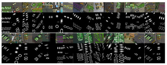
Figure 7.
Visualization of detection results in patches of the DOTA testing set. From top to bottom are two groups of detection results, center fields, and edge fields. For the images with multiple categories which correspond to several object fields, we only demonstrate one of them. The green line in the figure represents the elliptic field calculated by ERF. It is surrounded by a circumscribed rectangular box; namely, the oriented bounding box. Rectangular boxes of different colors represent different categories of targets.
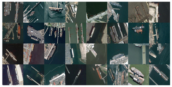
Figure 8.
Visualization of detection results from EFN in HRSC2016. The green line in the figure represents the elliptic field calculated by ERF. The red line denotes the circumscribed rectangle of the elliptical field.
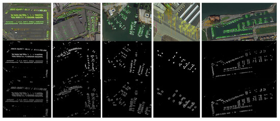
Figure 9.
Detection results in whole images of DOTA testing set. All of them have high resolution and cover a large area.
4.3. Comparison with the State-of-the-Art Methods
Table 1 shows a comparison of accuracy in DOTA. EFN outperformed the official baseline, FR-O [5], by 21.14 points and surpassed all of the state-of-the-art methods, demonstrating that our approach performs well in oriented object detection in aerial images. We argue that there are two reasons for this: (1) traditional frameworks first generate proposal boxes, then analyze boxes one by one, in order to discriminate whether a box is correct. It is easy to wrongly discriminate in this step. Meanwhile, EFN predicts fields, where the intensity of object regions is high while that of no-object regions is low, which is more similar to how the human visual system works. (2) Traditional frameworks regress bounding boxes. However, objects usually only occupy small parts of images, which makes these models more non-uniform. In comparison, EFN can better model the distributions of objects in aerial images by regressing fields. Although our method was originally designed for aerial image object detection, our experiments demonstrate that it also works well for conventional images and can be used in a variety of scenes with great potential. We also carried out a comparison in terms of memory, shown in Table 2. Traditional frameworks use deep backbones, such as ResNet [47], to extract features and rely on pre-trained models. As a consequence, such models are memory-consuming. EFN used U-Net as a backbone, which does not rely on a pre-trained model and is a relatively shallow backbone. Therefore, the model was much more memory efficient.

Table 1.
Comparison with the state-of-the-art methods on DOTA1.0. The short names for categories are defined as: PL, Plane; BD, Baseball diamond; BR, Bridge; GTF, Ground field track; SV, Small vehicle; LV, Large vehicle; SH, Ship; TC, Tennis court; BC, Basketball court; ST, Storage tank; SBF, Soccer-ball field; RA, Roundabout; HB, Harbor; SP, Swimming pool; and HC, Helicopter.
Table 2.
Comparison of memory use.
Table 3 shows the comparison of accuracy in HRSC2016. HRSC2016 contains many thin and long ship instances with arbitrary orientation. Based on our proposed method, the mAP reached 86.6, which was in line with the current state-of-the-art methods. As the visualization of the detection results shows, there were many ships arranged closely, which were long and narrow, making the horizontal rectangles hard to distinguish. In comparison, the proposed EFN method could effectively deal with this situation, thus proving the robust stability of our method.
Table 3.
Comparisons with the state-of-the-art methods on HRSC2016.
4.4. Ablation Study
In our research, we found that many factors had an impact on the performance of EFN. Therefore, we carried out an ablation study, considering various aspects, on DOTA. Specifically, we examined the cases of: (1) training the models with different input sizes; (2) using different backbones to construct EFN, whether to add batch normalization (BN) [52] after convolutional layers, and setting different batch sizes; and (3) training the models with different center field decay index and edge width .
Table 4 shows the accuracy and average testing speed comparison between different input sizes of EFN. Compared to EFN-112 and EFN-224, EFN-448 outperformed them, in terms of accuracy, to a great extent. EFN-576 achieved a higher mAP value, but the increase was modest and the test speed was much lower. Therefore, we considered that setting the input size to 448 * 448 was the most appropriate.
Table 4.
Accuracy and average testing speed comparison between different input sizes of EFN.
We chose two backbones: FCN [18] and U-Net. Based on the U-Net, we trained eight models using different batch sizes: four with BN and four without BN. The comparison is displayed in Table 5. From the table, it can be seen that U-Net achieved higher mAP. FCN is a sequential architecture, while there is a connection between the encoder and decoder in the U-Net; such a connection ensures that the gradient information can be passed directly to the upper layers, which helps gradient propagation and improves the network performance. Though the performance of the FCN backbone was inferior to that of U-Net, it still outperformed many prior works. This indicates that the EFN is compatible with different backbones and improves the detection performance.
Table 5.
Comparison of models trained with different configurations. All models were trained using an input size of 224 × 224. “√” means adding batch normalization after convolutional layers.
U-Net with BN performed better than that without, as BN can reduce overfitting, avoid the gradient vanishing problem, and accelerate training. To a certain extent, a larger batch size results in better performance but consumes more memory. Further experiments found that training with small batch size in the preliminary phase, then with larger batch size was an effective strategy. The small batch size makes for faster convergence, while the larger batch size makes for finer optimization.
There are two critical parameters in the training phase: the center field decay index and the edge width . These two parameters both have significant impact on the performance. To find the best values, we trained models using a range of values. Table 6 shows a comparison of models trained with different and . Both of them should be set to appropriate values. If the value of is too low, the CF decays suddenly from the center to edge, which may cause the wrong object center to be found in the ERF. A too-high value of causes the CF to decay rapidly, leading to difficulties in detecting the object center. A low value of will make the EF inconspicuous. In this case, the detection of points on the edge will be inaccurate and some points may be left out. A high value of may cause the edge overlap of adjacent objects, which will bring about disturbances for the edge distinction of different objects. In our experiments, we found that setting to 2.5 and to 0.1 achieved high performance, which thus served as the default values.
Table 6.
Comparison of models trained with different and values. All models were trained with an input size of 224 × 224. The batch size was set to 64.
4.5. Experiments on Natural Images
To verify the universality of our model, we further tested the proposed techniques on generic data sets: the PASCAL VOC 2012 challenge [45]. We used the VOC2007 train+val+test sets (9963 images) and VOC2012 train+val sets (11,540 images) to train the network and then used the VOC2012 test sets for testing. Unlike the aerial images, the VOC images are in the low altitude perspective and are of low resolution. Thus, we no longer cropped the images or predicted the angle of the object. In other words, we only predicted four parameters and simply pre-defined , as shown in Equation (10). Table 7 shows the results. We achieved 84.7% mAP. A visualization of detection results is shown in Figure 10. Compared to the state-of-the-art methods, EFN (which specializes in different application scenarios) still obtained good scores.
Table 7.
Comparison with prior works on VOC 2012. All methods were trained on VOC 2007 and VOC 2012 trainval sets plus the VOC 2007 test set, and were tested on the VOC 2012 test set.
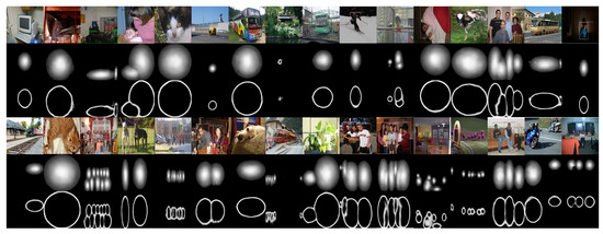
Figure 10.
Visualization of detection results in patches of the PASCAL VOC testing set. From top to bottom are two groups of detection results, center fields, and edge fields. For the images with multiple categories corresponding to several object fields, we only demonstrate one of them.
5. Conclusions
In this paper, we proposed a novel method for detecting objects in aerial images with oriented bounding boxes. Unlike typical region proposal and semantic segmentation methods, we introduced the field concept into our work, using a remoulded FCN network to calculate the center field and edge field. Then, we used the robust ellipse region fitting algorithm to precisely identify objects. This is a pixel-wise framework using patch-wise annotation, which dramatically reduces the difficulty of network training. Experiments on the DOTA and HRSC2016 data sets showed that EFN can outperform many prior methods, in terms of both speed and accuracy. In the DOTA test set, the mAP of our method reached 75.72; 2.66 higher than the second place. In the HRSC2016 test set, our method also achieved 86.6, the best mAP. Although our test on VOC2012 was not the best, it was only 0.7 less than the first place, verifying the generality of our techniques. Furthermore, we carried out an ablation study, discussed how different factors influence the performance of EFN, and found an appropriate way to train it. In the future, we intend to carry out more research on EFN and to continuously improve our method.
Author Contributions
Conceptualization, J.L.; methodology, J.L.; software, J.L.; validation, J.L.; formal analysis, J.L. and H.Z.; writing—original draft preparation, H.Z.; writing—review and editing, J.L. and H.Z.; visualization, H.Z.; supervision, J.L.; project administration, J.L. All authors have read and agreed to the published version of the manuscript.
Funding
This research was funded by National Natural Science Foundation of China under Grant No. 41271454.
Conflicts of Interest
The authors declare no conflict of interest.
References
- Cheng, G.; Zhou, P.; Han, J. Learning Rotation-Invariant Convolutional Neural Networks for Object Detection in VHR Optical Remote Sensing Images. IEEE Trans. Geosci. Remote Sens. 2016, 54, 7405–7415. [Google Scholar] [CrossRef]
- Long, Y.; Gong, Y.; Xiao, Z.; Liu, Q. Accurate object localization in remote sensing images based on convolutional neural networks. IEEE Trans. Geosci. Remote Sens. 2017, 55, 2486–2498. [Google Scholar] [CrossRef]
- Wang, G.; Wang, X.; Fan, B.; Pan, C. Feature extraction by rotation-invariant matrix representation for object detection in aerial image. IEEE Geosci. Remote Sens. Lett. 2017, 14, 851–855. [Google Scholar] [CrossRef]
- Deng, Z.; Sun, H.; Zhou, S.; Zhao, J.; Zou, H. Toward fast and accurate vehicle detection in aerial images using coupled region-based convolutional neural networks. IEEE J. Sel. Top. Appl. Earth Obs. Remote Sens. 2017, 10, 3652–3664. [Google Scholar] [CrossRef]
- Xia, G.S.; Bai, X.; Ding, J.; Zhu, Z.; Belongie, S.; Luo, J.; Datcu, M.; Pelillo, M.; Zhang, L. DOTA: A large-scale dataset for object detection in aerial images. In Proceedings of the IEEE Conference on Computer Vision and Pattern Recognition, Salt Lake City, UT, USA, 18–22 June 2018; pp. 3974–3983. [Google Scholar]
- Hsieh, M.R.; Lin, Y.L.; Hsu, W.H. Drone-based object counting by spatially regularized regional proposal network. In Proceedings of the IEEE International Conference on Computer Vision, Venice, Italy, 22–29 October 2017; pp. 4145–4153. [Google Scholar]
- Girshick, R.; Donahue, J.; Darrell, T.; Malik, J. Rich feature hierarchies for accurate object detection and semantic segmentation. In Proceedings of the IEEE Conference on Computer Vision and Pattern Recognition, Columbus, OH, USA, 23–28 June 2014; pp. 580–587. [Google Scholar]
- Girshick, R. Fast r-cnn. In Proceedings of the IEEE International Conference on Computer Vision, Cambridge, MA, USA, 20–23 June 1995; pp. 1440–1448. [Google Scholar]
- Ren, S.; He, K.; Girshick, R.; Sun, J. Faster r-cnn: Towards real-time object detection with region proposal networks. In Proceedings of the Advances in Neural Information Processing Systems, Montreal, QC, Canada, 7–12 December 2015; pp. 91–99. [Google Scholar]
- Xiao, Z.; Gong, Y.; Long, Y.; Li, D.; Wang, X.; Liu, H. Airport detection based on a multiscale fusion feature for optical remote sensing images. IEEE Geosci. Remote Sens. Lett. 2017, 14, 1469–1473. [Google Scholar] [CrossRef]
- Li, X.; Wang, S. Object detection using convolutional neural networks in a coarse-to-fine manner. IEEE Geosci. Remote Sens. Lett. 2017, 14, 2037–2041. [Google Scholar] [CrossRef]
- Liu, Z.; Wang, H.; Weng, L.; Yang, Y. Ship rotated bounding box space for ship extraction from high-resolution optical satellite images with complex backgrounds. IEEE Geosci. Remote Sens. Lett. 2016, 13, 1074–1078. [Google Scholar] [CrossRef]
- Liu, K.; Mattyus, G. Fast Multiclass Vehicle Detection on Aerial Images. IEEE Geosci. Remote Sens. Lett. 2015, 12, 1938–1942. [Google Scholar] [CrossRef]
- Yang, X.; Sun, H.; Fu, K.; Yang, J.; Sun, X.; Yan, M.; Guo, Z. Automatic ship detection in remote sensing images from google earth of complex scenes based on multiscale rotation dense feature pyramid networks. Remote Sens. 2018, 10, 132. [Google Scholar] [CrossRef]
- Zhang, Z.; Guo, W.; Zhu, S.; Yu, W. Toward arbitrary-oriented ship detection with rotated region proposal and discrimination networks. IEEE Geosci. Remote Sens. Lett. 2018, 15, 1745–1749. [Google Scholar] [CrossRef]
- Ding, J.; Xue, N.; Long, Y.; Xia, G.S.; Lu, Q. Learning roi transformer for oriented object detection in aerial images. In Proceedings of the IEEE Conference on Computer Vision and Pattern Recognition, Long Beach, CA, USA, 15–20 June 2019; pp. 2849–2858. [Google Scholar]
- Yang, X.; Yang, J.; Yan, J.; Zhang, Y.; Zhang, T.; Guo, Z.; Sun, X.; Fu, K. Scrdet: Towards more robust detection for small, cluttered and rotated objects. In Proceedings of the IEEE International Conference on Computer Vision, Seoul, Korea, 27 October–2 November 2019; pp. 8232–8241. [Google Scholar]
- Long, J.; Shelhamer, E.; Darrell, T. Fully convolutional networks for semantic segmentation. In Proceedings of the IEEE conference on computer vision and pattern recognition, Boston, MA, USA, 7–12 June 2015; pp. 3431–3440. [Google Scholar]
- Ji, S.; Wei, S.; Lu, M. Fully Convolutional Networks for Multisource Building Extraction From an Open Aerial and Satellite Imagery Data Set. IEEE Trans. Geosci. Remote Sens. 2019, 57, 574–586. [Google Scholar] [CrossRef]
- Dickenson, M.; Gueguen, L. Rotated Rectangles for Symbolized Building Footprint Extraction. In Proceedings of the 2018 IEEE/CVF Conference on Computer Vision and Pattern Recognition Workshops (CVPRW), Salt Lake City, UT, USA, 18–22 June 2018; pp. 215–2153. [Google Scholar] [CrossRef]
- Xu, Y.; Wu, L.; Xie, Z.; Chen, Z. Building extraction in very high resolution remote sensing imagery using deep learning and guided filters. Remote Sens. 2018, 10, 144. [Google Scholar] [CrossRef]
- Yuan, J. Learning building extraction in aerial scenes with convolutional networks. IEEE Trans. Pattern Anal. Mach. Intell. 2017, 40, 2793–2798. [Google Scholar] [CrossRef] [PubMed]
- Liang, J.; Homayounfar, N.; Ma, W.C.; Wang, S.; Urtasun, R. Convolutional recurrent network for road boundary extraction. In Proceedings of the IEEE Conference on Computer Vision and Pattern Recognition, Long Beach, CA, USA, 15–20 June 2019; pp. 9512–9521. [Google Scholar]
- Cheng, G.; Wang, Y.; Xu, S.; Wang, H.; Xiang, S.; Pan, C. Automatic road detection and centerline extraction via cascaded end-to-end convolutional neural network. IEEE Trans. Geosci. Remote Sens. 2017, 55, 3322–3337. [Google Scholar] [CrossRef]
- Bastani, F.; He, S.; Abbar, S.; Alizadeh, M.; Balakrishnan, H.; Chawla, S.; Madden, S.; DeWitt, D. Roadtracer: Automatic extraction of road networks from aerial images. In Proceedings of the IEEE Conference on Computer Vision and Pattern Recognition, Salt Lake City, UT, USA, 18–22 June 2018; pp. 4720–4728. [Google Scholar]
- Lu, X.; Zhong, Y.; Zheng, Z.; Liu, Y.; Zhao, J.; Ma, A.; Yang, J. Multi-scale and multi-task deep learning framework for automatic road extraction. IEEE Trans. Geosci. Remote Sens. 2019, 57, 9362–9377. [Google Scholar] [CrossRef]
- Batra, A.; Singh, S.; Pang, G.; Basu, S.; Jawahar, C.; Paluri, M. Improved road connectivity by joint learning of orientation and segmentation. In Proceedings of the IEEE Conference on Computer Vision and Pattern Recognition, Long Beach, CA, USA, 15–20 June 2019; pp. 10385–10393. [Google Scholar]
- Mou, L.; Zhu, X.X. Vehicle instance segmentation from aerial image and video using a multitask learning residual fully convolutional network. IEEE Trans. Geosci. Remote Sens. 2018, 56, 6699–6711. [Google Scholar] [CrossRef]
- Zhang, C.; Sargent, I.; Pan, X.; Li, H.; Gardiner, A.; Hare, J.; Atkinson, P.M. An object-based convolutional neural network (OCNN) for urban land use classification. Remote Sens. Environ. 2018, 216, 57–70. [Google Scholar] [CrossRef]
- Huang, B.; Zhao, B.; Song, Y. Urban land-use mapping using a deep convolutional neural network with high spatial resolution multispectral remote sensing imagery. Remote Sens. Environ. 2018, 214, 73–86. [Google Scholar] [CrossRef]
- Zhang, C.; Sargent, I.; Pan, X.; Li, H.; Gardiner, A.; Hare, J.; Atkinson, P.M. Joint Deep Learning for land cover and land use classification. Remote Sens. Environ. 2019, 221, 173–187. [Google Scholar] [CrossRef]
- Cai, Z.; Vasconcelos, N. Cascade r-cnn: Delving into high quality object detection. In Proceedings of the IEEE Conference on Computer Vision and Pattern Recognition, Salt Lake City, UT, USA, 18–22 June 2018; pp. 6154–6162. [Google Scholar]
- Cao, Z.; Hidalgo, G.; Simon, T.; Wei, S.E.; Sheikh, Y. OpenPose: Realtime multi-person 2D pose estimation using Part Affinity Fields. arXiv 2018, arXiv:1812.08008. [Google Scholar] [CrossRef]
- Newell, A.; Yang, K.; Deng, J. Stacked hourglass networks for human pose estimation. In Proceedings of the 14th European Conference on Computer Vision, Amsterdam, The Netherlands, 8–16 October 2016; Springer: Cham, Switzerland, 2016; pp. 483–499. [Google Scholar]
- Brahmbhatt, S.; Christensen, H.I.; Hays, J. StuffNet: Using ‘Stuff’ to improve object detection. In Proceedings of the 2017 IEEE Winter Conference on Applications of Computer Vision (WACV), Santa Rosa, CA, USA, 24–31 March 2017; IEEE: Piscataway, NJ, USA, 2017; pp. 934–943. [Google Scholar]
- Shrivastava, A.; Gupta, A. Contextual priming and feedback for faster r-cnn. In Proceedings of the 14th European Conference on Computer Vision, Amsterdam, The Netherlands, 8–16 October 2016; Springer: Cham, Switzerland, 2016; pp. 330–348. [Google Scholar]
- Gidaris, S.; Komodakis, N. Object detection via a multi-region and semantic segmentation-aware cnn model. In Proceedings of the IEEE International Conference on Computer Vision, Santiago, Chile, 7–13 December 2015; pp. 1134–1142. [Google Scholar]
- Bell, A.J.; Sejnowski, T.J. The “independent components” of natural scenes are edge filters. Vis. Res. 1997, 37, 3327–3338. [Google Scholar] [CrossRef]
- Olshausen, B.A.; Field, D.J. Emergence of simple-cell receptive field properties by learning a sparse code for natural images. Nature 1996, 381, 607–609. [Google Scholar] [CrossRef] [PubMed]
- Luo, W.; Li, Y.; Urtasun, R.; Zemel, R. Understanding the effective receptive field in deep convolutional neural networks. In Proceedings of the Advances in Neural Information Processing Systems, Barcelona, Spain, 5–10 December 2016; pp. 4898–4906. [Google Scholar]
- Soong, T.T. Fundamentals of Probability and Statistics for Engineers; John Wiley & Sons: Hoboken, NJ, USA, 2004. [Google Scholar]
- Ronneberger, O.; Fischer, P.; Brox, T. U-net: Convolutional networks for biomedical image segmentation. In Proceedings of the International Conference on Medical Image Computing and Computer-Assisted Intervention, Munich, Germany, 5–9 October 2015; Springer: Cham, Switzerland, 2015; pp. 234–241. [Google Scholar]
- Neubeck, A.; Van Gool, L. Efficient non-maximum suppression. In Proceedings of the 18th International Conference on Pattern Recognition (ICPR’06), Hong Kong, China, 20–24 August 2006; IEEE: Piscataway, NJ, USA, 2006; Volume 3, pp. 850–855. [Google Scholar]
- Ma, C.; Jiang, L. Some research on Levenberg—Marquardt method for the nonlinear equations. Appl. Math. Comput. 2007, 184, 1032–1040. [Google Scholar] [CrossRef]
- Everingham, M.; Van Gool, L.; Williams, C.K.I.; Winn, J.; Zisserman, A. The PASCAL Visual Object Classes Challenge 2012 (VOC2012) Results. Available online: http://www.pascal-network.org/challenges/VOC/voc2012/workshop/index.html (accessed on 22 January 2019).
- Redmon, J. Darknet: Open Source Neural Networks in C. 2013. Available online: https://pjreddie.com/darknet (accessed on 28 October 2020).
- He, K.; Zhang, X.; Ren, S.; Sun, J. Deep residual learning for image recognition. In Proceedings of the IEEE Conference on Computer Vision and Pattern Recognition, Las Vegas, NV, USA, 27–30 June 2016; pp. 770–778. [Google Scholar]
- Ma, J.; Shao, W.; Ye, H.; Wang, L.; Wang, H.; Zheng, Y.; Xue, X. Arbitrary-oriented scene text detection via rotation proposals. IEEE Trans. Multimed. 2018, 20, 3111–3122. [Google Scholar] [CrossRef]
- Jiang, Y.; Zhu, X.; Wang, X.; Yang, S.; Li, W.; Wang, H.; Fu, P.; Luo, Z. R2cnn: Rotational region cnn for orientation robust scene text detection. arXiv 2017, arXiv:1706.09579. [Google Scholar]
- Yang, X.; Sun, H.; Sun, X.; Yan, M.; Guo, Z.; Fu, K. Position detection and direction prediction for arbitrary-oriented ships via multitask rotation region convolutional neural network. IEEE Access 2018, 6, 50839–50849. [Google Scholar] [CrossRef]
- Liao, M.; Zhu, Z.; Shi, B.; Xia, G.s.; Bai, X. Rotation-sensitive regression for oriented scene text detection. In Proceedings of the IEEE conference on computer vision and pattern recognition, Salt Lake City, UT, USA, 18–22 June 2018; pp. 5909–5918. [Google Scholar]
- Normalization, B. Accelerating deep network training by reducing internal covariate shift. arXiv 2015, arXiv:abs/1502.03167. [Google Scholar]
- Shrivastava, A.; Gupta, A.; Girshick, R. Training region-based object detectors with online hard example mining. In Proceedings of the IEEE Conference on Computer Vision and Pattern Recognition, Las Vegas, NV, USA, 27–30 June 2016; pp. 761–769. [Google Scholar]
- Dai, J.; Li, Y.; He, K.; Sun, J. R-fcn: Object detection via region-based fully convolutional networks. In Proceedings of the Advances in Neural Information Processing Systems, Barcelona, Spain, 5–10 December 2016; pp. 379–387. [Google Scholar]
- Liu, W.; Anguelov, D.; Erhan, D.; Szegedy, C.; Reed, S.; Fu, C.Y.; Berg, A.C. Ssd: Single shot multibox detector. In Proceedings of the European Conference on Computer Vision, Amsterdam, The Netherlands, 8–16 October 2016; Springer: Cham, Switzerland, 2016; pp. 21–37. [Google Scholar]
- Zhang, S.; Wen, L.; Bian, X.; Lei, Z.; Li, S.Z. Single-shot refinement neural network for object detection. In Proceedings of the IEEE Transactions on Circuits and Systems for Video Technology, Salt Lake City, UT, USA, 18–23 June 2018. [Google Scholar]
- Zhao, H.; Shi, J.; Qi, X.; Wang, X.; Jia, J. Pyramid scene parsing network. In Proceedings of the IEEE conference on computer vision and pattern recognition, Honolulu, HI, USA, 21–26 July 2017; pp. 2881–2890. [Google Scholar]
Publisher’s Note: MDPI stays neutral with regard to jurisdictional claims in published maps and institutional affiliations. |
© 2020 by the authors. Licensee MDPI, Basel, Switzerland. This article is an open access article distributed under the terms and conditions of the Creative Commons Attribution (CC BY) license (http://creativecommons.org/licenses/by/4.0/).