Abstract
Number comparison has long been recognized as one of the most fundamental non-modular arithmetic operations to be executed in a non-positional Residue Number System (RNS). In this paper, a new technique for designing comparators of RNS numbers represented in an arbitrary moduli set is presented. It is based on a newly introduced modified diagonal function, whose strictly monotonic properties make it possible to replace the cumbersome operations of finding the remainder of the division by a large and awkward number with significantly simpler computations involving only a power of 2 modulus. Comparators of numbers represented in sample RNSs composed of varying numbers of moduli and offering different dynamic ranges, designed using various methods, were synthesized for the 65 nm technology. The experimental results suggest that the new circuits enjoy a delay reduction ranging from over 11% to over 75% compared to the fastest circuits designed using existing methods. Moreover, it is achieved using less hardware, the reduction of which reaches over 41%, and is accompanied by significantly reduced power-consumption, which in several cases exceeds 100%. Therefore, it seems that the presented method leads to the design of the most efficient current hardware comparators of numbers represented using a general RNS moduli set.
1. Introduction
Parallel data processing is one of the most viable approaches to meet steadily growing needs for high-performance computations. Therefore, algorithms and data representations enjoying parallel structures, which facilitate the processing of a large amount of data efficiently, have been an area of active research for many years. One of the promising directions in this field relies on using the Residue Number System (RNS) to represent integers [1,2]. The RNS is a non-positional number system defined by the set of () pairwise relatively prime positive integers called moduli . Its dynamic range is equal to the product , which allows it to represent all -bit numbers, where . Any non-negative integer such that can be uniquely represented in RNS as , where the ith digit of in RNS is the remainder of the integer division of by the modulus , represented in bits.
Indeed, in recent years, an inherent parallelism between RNS and potentially lower power consumption has motivated researchers to consider its use for implementation in hardware of various classes of computations, like digital filtering [3,4,5,6], multicarrier modulation schemes with error correction [7], and some cryptographic algorithms [8]. An excellent summary of other RNS applications for Digital Signal Processing (DSP) systems and analysis of various design issues can be found in [9]. Coprocessors with limited sets of instructions for high-speed and low power consumption executed in RNS have been proposed [10,11]. Besides these well-established applications, many other emerging RNS applications have been surveyed [12].
The primary benefit of RNS is the possibility of parallel execution of basic arithmetic operations (addition, subtraction, and multiplication). Unlike positional number representation, the RNS is carry-free, which can simplify the processing of large numbers, replacing it with the execution of parallel arithmetic modular operations on numbers of significantly smaller size. Unfortunately, several non-modular operations are also indispensable, the execution of which in RNS requires interaction between different moduli due to the positional nature of these operations: residue-to-binary (reverse) conversion, magnitude comparison, sign detection, overflow detection, scaling, and division. Among them, magnitude comparison is one of the most fundamental operations, and it, besides being used directly, is also the cornerstone of division, sign detection, overflow detection, etc. Unfortunately, it is a difficult operation in RNS, because a non-positional RNS number representation does not reveal any information about the magnitude of a number, so that special methods involving handling all residue digits must be used.
Several techniques for number comparison in RNS have been studied [1,13,14,15,16,17,18,19,20,21,22,23,24,25]. The simplest approach to comparing numbers in RNS relies on first converting them to the positional notation, just to be compared using a simple number comparator [1]. Such a comparator is based on using any reverse (residue-to-binary) converter, which can be built on the basis of the Chinese Remainder Theorem (CRT), the Mixed Radix Conversion (MRC) method, or some variant or a combination of them [1,2,26,27,28]. Because the reverse converter is available anyway in any RNS-based processor, the only extra hardware cost is that of the ordinary -bit comparator of numbers, which can be designed, e.g., according to [29] (pp. 45–47). Obviously, a comparison relying on traditional reverse conversion techniques inherits their major drawbacks: the multi-operand addition modulo is a large number (the dynamic range ) for the CRT or lengthy sequential computations for the MRC, either resulting in excessive delay and unnecessarily high power consumption.
One of the most promising approaches to handle non-positional arithmetic operations in RNS that has been proposed relies on computation of some positional characteristics of RNS numbers, according to which it would be possible to determine the magnitudes of numbers and hence their comparison. This idea relies on a hypothesis that computations involving such a positional characteristic can be implemented more efficiently than reverse conversion, due to using simpler arithmetic operations. One is the core function introduced in 1977 by Akushskii [13] and used for comparison. Its faster version, making it possible to avoid lengthy iterative computations, relied on introducing a redundant modulus and was proposed in [14]. The other approach uses the so-called diagonal function, which is defined as the sum of the quotients of division of the number by all system moduli, introduced in [16] and further developed in [18] and [21]. One of the methods based on the diagonal function, called the Sum of Quotients Technique (SQT), was claimed to be one of the most efficient hardware approaches [18]. Unfortunately, a more accurate performance estimation of the latter, presented recently in [23], revealed that the direct implementation of the comparator using the diagonal function according to [16,18] leads to inefficient circuitry. (Because the design method proposed here is based on some ideas of the diagonal function, while aiming to avoid its drawbacks, it will be detailed in Section 2.) Some other general approaches to RNS number comparison were presented in [15,17,22,26,27]. In [15], a comparison was proposed based on parity checking, provided that the basic moduli set consists of odd moduli only and that the redundant modulus is added. Those proposed in [26,27] make it possible to compute the positional characteristic using CRT without the expensive operation of finding the remainder of a division. The comparison algorithm based on the new CRT-II, suggested in [17], makes it possible to reduce the maximum size of the modulo addition from to approximately , where is the dynamic range. The method of [22] relies on the approximate calculation of positional numbers according to CRT, whereas that of [24] makes it possible to compare signed numbers, but it also requires sign detection for each compared number. Finally, some comparators have been proposed for RNSs using special bases, e.g., the 4-moduli set composed of two pairs of conjugate moduli , as well as the 3-moduli sets [20] and [25].
In summary, the drawbacks of the previous magnitude comparison algorithms are: the need for using a redundant modulus, restricting the moduli set or time-consuming modulo operations involving large numbers (the size of the dynamic range or close). Here we will show how to extend the idea of diagonal function so that a high-speed and efficient comparator in RNS can be implemented in hardware. The new approach proposed here relies on integrating techniques from [16,26], and it is based on modifying the diagonal function of the numbers represented in RNS. The major advantages of this method are that, in addition to not requiring the computation of a remainder of division, it also leads to computations involving numbers of smaller sizes than in [26].
This paper is organized as follows. Section 2 presents the method of comparison using the SQT based on the diagonal function. Section 3 thoroughly details the theoretical background of the modified diagonal function proposed here, leading to significantly improved performance of the comparator. Performance estimations and comparison against existing circuits are provided in Section 4. Finally, some conclusions and suggestions for future research are given in Section 5.
2. Number Comparison Using the Sum of Quotients Technique (SQT)
In this section, we will present all key ideas related to the SQT method of [16], which will facilitate understanding of our method relying on a modification of the SQT method, which will be presented in Section 3. The main idea of the SQT method relies on the observation that in the finite -dimensional space determined by the number of moduli , the integers are ordered along straight lines, which are parallel to the main diagonal of the space. In MRC, each line represents the most significant digit of the number. However, these diagonals can be renumbered in a natural order of integers. In this case, the comparison of two numbers can be done by considering the numbers of the diagonals to which they belong. For fast determination of the diagonal to which a number belongs, a monotonically increasing function called the Sum of Quotients (SQ) was defined:
where . Let us define the following constant:
where is the multiplicative inverse of mod , i.e., such an integer that . (Recall that a multiplicative inverse exists provided that and are co-prime, which is indeed the case here.) It was shown that for the set of constants the following congruence holds:
These notions are essential to defining the diagonal function as
which was shown to be monotonically increasing over a set of integers . This method is called the Sum of Quotients Technique (SQT), because the following important equality holds:
The comparison of RNS numbers using SQT is summarized in the following algorithm, whose hardware implementation is shown in Figure 1.
| Algorithm 1: Comparison of RNS numbers using SQT. |
| Input: , Output: “100” if , “010” if , and “001” if . Step 1. Calculate and . Note: These computations are independent and therefore they can be executed in parallel, provided that two circuits implementing the diagonal function are available. Step 2. Compare the values of and : 1. if then return “100”; 2. if then return “001”; 3. if then: 3.1. if then return “100”; 3.2. if then return “010”; 3.3. if then return “001”. |
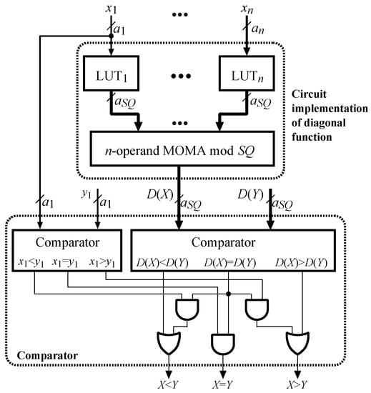
Figure 1.
Hardware implementation of the basic number comparison algorithm using the diagonal function [25,28].
The main disadvantage of Algorithm 1 is that the computation of the remainder of the division over the modulus , executed by the -operand multi-operand modular adder (MOMA) mod , is both hardware and time-consuming. (It will be seen later that for sample moduli sets the difference between the bit sizes of and could be from 3 to 5-bits.) In [16], it was suggested that in the case of the equality (the diagonal function is not strictly monotonic), an extra comparison must be executed. However, in [23], it was shown that this additional comparison can actually be done in parallel, so that the only delay penalty is two gate levels (this observation was taken into account in Figure 1). In the following section, we will show how to modify SQT to replace the MOMA mod with a significantly faster and simpler circuit modulo with a power of 2.
3. Comparison Using the Modified Diagonal Function
Here, we will describe the new method for comparison of RNS numbers based on introducing the modified diagonal function (MDF). It is based on the observation that if all constants are divided by , i.e., similarly as was done for the CRT-based sign detector proposed in [26], then it is possible to move the computations from the residue class to the computations in the interval , so that computations involving integer parts of real numbers are not really needed. In other words, the operation of finding the remainder of the division by is replaced with the more efficient operation of discarding an integer part of a number. However, the major concern with such an approach is its accuracy, because in most cases the fractional numbers cannot be represented exactly using a finite number of bits. Nevertheless, the accurate passing from computations on fraction parts to computations on integers can be done as follows:
- Multiply each real constant by , where is the number of bits of the fraction part, which guarantees sufficient accuracy.
- For each real number, say , calculate , i.e., the smallest integer not less than .
- Execute all computations modulo (it is sufficient to ignore all carries generated from the -th position).
Note: The only limitation for the above conversion could occur when divides (i.e., is a power of two), because in this case, the method suggested reduces to the original one. Nevertheless, because in most cases does not divide , we will therefore henceforth consider only this case. To determine the smallest which guarantees sufficient accuracy, we proceed as follows.
First, notice that the constants can be recalculated as
where and . Because according to Equality (3) the sum is divisible by , it implies that is an integer. Furthermore, because then .
Now we can define the following positional characteristic of a number, which will be called the modified diagonal function (MDF):
Theorem 1.
Letbe the largest modulus of the moduli set. Ifthen the MDFis strictly increasing for any, i.e., for anywe have.
Proof.
First, we find the value of for any . Because for any
therefore, according to Equality (5), we have
where
Consider
where denotes discarding of an integer part of . Obviously, because , can be determined using Equality (10):
Now we will determine the properties of the functions and . By applying the notation introduced earlier, we obtain
which leads to
Now according to Equality (11) and by taking into account that in RNS , we obtain
Because for any
in Equality (14) we have
which hence becomes
From the formulas derived above, it is obvious that is the additional term of the expression equal to
By considering that
we obtain
For the function to be strictly increasing, it is necessary to satisfy the two following conditions.
Condition 1.
This inequality makes it possible to pass from computation of the remainder of the division to the computation for in Equality (13), and hence in Equality (16) as well.
Condition 2.
If this inequality holds and both Condition 1 and Inequality (19) are satisfied, it implies that the value of calculated by Equality (13) is larger than the value of calculated by Equality (16).
Whether any of these two conditions is satisfied, it depends on . Now we will show how to determine the smallest , for which both Conditions 1 and 2 hold. As the function is monotonic, hence . Thus, according to Equality (2)
Additionally, because and , therefore
Because Condition 1 leads to the inequality
therefore
which in turn leads to , and finally to
From Condition 1, and assuming that Inequality (24) holds, we have
Now consider the inequality
If the inequality
holds for , then Inequality (26) is true for with any number of zeros in its RNS representation. Therefore, we can estimate from Inequality (27). Recalling that , , and , therefore
which implies that Inequality (27) holds if
To estimate , we calculate the logarithm of the last inequality
which is identical to Inequality (24). Therefore, if Inequality (24) holds, then both Conditions 1 and 2 are satisfied, which concludes the proof. □
Inequality (24) can be considered as the condition that guarantees strict monotonicity of the MDF : if it holds, to compare two RNS numbers and , it suffices to compare the values of and . The above considerations can be formally summarized as the following algorithm.
| Algorithm 2: Comparison of RNS numbers using MDF. |
| Input:, Output: “100” if , “010” if , and “001” if . Step 1. Calculate and . Note: These computations are independent and therefore they can be executed in parallel, provided that two circuits implementing the MDF are available. Step 2. Compare the values of and . 1. if then return “100” 2. if then return “001” 3. if then return “010” |
In summary, the diagonal function of [16,18] is monotonic for , whereas the MDF proposed here is strictly monotonic over this set (which makes it possible to compare numbers directly).
The differences between and are illustrated for a sample 3-moduli RNS {5, 11, 17}. Figure 2 shows the diagrams of the values of the functions and for the first 15 values of , which clearly reflect their monotonic properties and demonstrate their differences.
Example 1.
Consider a sample set ofmoduli,, nadwhose dynamic range is. Here, we have,,, which implies, so thatand the four constants
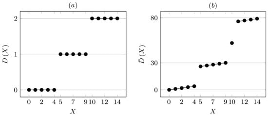
Figure 2.
Values of the functions for : (a) and (b) .
Let us compare three integers
for which we have
Recall that according to Theorem 1, the function is strictly monotonic for any . Indeed, it is seen that: (i) implies and (ii) implies .
Figure 3 shows the general scheme of the new comparator that implements Algorithm 2 (here ). Obviously, it is necessary to add more extra hardware than its simple counterpart using any reverse converter followed by the -bit comparator, because only the latter small circuit must be added to the RNS-based processor. In our circuit, both the circuit computing and the -bit comparator must be added. Nevertheless, the new comparator has two potential major advantages over the latter: (i) higher speed, because of the delay of the -operand MOMA mod is certainly significantly smaller than of the n-operand MOMA mod [30,31] in the CRT-based version of the reverse converter or of its MRC-based version (a slightly larger size of the operands handled by the final -bit comparator ( vs. ) has little impact on the area or delay of the final -bit comparator); and (ii) lower power consumption, because of the significantly smaller circuitry involved in performing the comparison. Either claim will be confirmed by performance estimations obtained for ASIC implementations of various basic general RNS number comparators, presented in the next section.
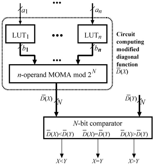
Figure 3.
Hardware implementation of the new comparator built using the MDF.
4. Performance Estimations
In this section, we first present an approximate evaluation of the performance of hardware implementations of the new general RNS comparators and their three best-known counterparts, and then we provide more accurate estimations for ASIC implementations of all circuits considered.
Suppose that all n RNS moduli are l-bit numbers. Then, the basic parameters of operands involved in modulo operations handled by four general RNS number comparators can be summarized as listed in Table 1. First, recall that all these circuits have a number of steps growing logarithmically in the function of the number of moduli , i.e., they all have delay. Second, notice that the following inequalities hold: and . The three circuits based on the CRT, SQT, and MDF have a similar structure, composed of the n-operand modulo adder, with the major difference made by the modulus. Because neither nor is a power of 2 and , then it seems that the SQT-based circuit should involve less hardware and be faster than the CRT-based one. On the other hand, because the MDF-based circuit proposed here uses the n-operand adder modulo a power of 2 (), it enjoys the major advantage of all arithmetic circuits mod : significantly smaller delay and exceptional hardware efficiency compared to all its counterparts modulo any odd modulus involving cumbersome and lengthy operations of finding the remainder of the division by a large and awkward number or . The simplicity and the speed gained by the latter outweighs the minor delay/area differences due to a slightly larger final comparator of -bit vs. a-bit and -bit numbers. As for the comparator based on the CRT-II of [17] it executes iterative steps on operands of growing size and involving computations modulo a size growing up to about . On one hand, is not only the smallest of the moduli involved in computations by all comparators considered, but it is also involved only in the final stage of iterative computations, which suggests that it would result in some advantages. On the other hand, the estimation of delay/area performance of this circuit is difficult, because each iterative step involves modulo computations which, despite being executed on relatively small size moduli are nevertheless time-consuming and executed serially.

Table 1.
Summary of basic parameters of four RNS comparison methods for general moduli sets.
To obtain more accurate complexity estimations, we synthesized all four comparators described above for various RNS moduli sets, which are grouped into two classes, listed in Table 2. Class 1 consists of 4-moduli sets; each set composed of moduli of the same size . Varying the size of moduli makes it possible to observe comparators’ performance in the function of the dynamic range , which grows only with the size of the moduli but not with their number (which remains constant). Class 2 consists of moduli of the same size (we chose bits), whose number varies from 3 to 8, allowing to observe comparators’ performance in the function of the number of moduli. All sets of selected moduli consist of the largest existing pairwise prime moduli for a given .
Table 2.
Sample sets of moduli and their characteristics.
The circuits were described in parametrized structural VHDL following identical coding guidelines and synthesized following the similar layout of module hierarchy and primitive components like adders. The additions and multiplications were implemented with register-transfer level (RTL) operators and selection of their architectures was left to be done by the synthesis tool. We performed logic synthesis of the comparators for a range of target moduli sets using Cadence RTL Compiler v. 8.1 and an industrial 65 nm low-power library (STM CMOS065LP). For each design and moduli set, the minimum delay was found, which we assumed to be the smallest delay target when the synthesis was still able to achieve a non-negative timing slack. The cell area and total power (including dynamic and leakage components) reported by the synthesis tool were given an area and power figures.
The complexity characteristics obtained are detailed in Table 3, Table 4, Table 5, Table 6, Table 7 and Table 8 and visualized in Figure 4 and Figure 5. It can be seen that the delay of the new comparator proposed here grows equally slowly (almost linearly) while increasing the dynamic range or the number of moduli . It seems that it results directly from the possibility of replacing cumbersome operations of finding the remainder of the division by a large and awkward number with significantly simpler multi-operand additions mod . The synthesis results suggest that the new comparator proposed here is faster than all known similar circuits for all sample moduli sets considered, with delay reduction ranging from over 11% to over 75% compared to the fastest circuit designed using existing methods. Only the basic CRT-based implementation introduces delay slightly larger but only in a few cases. The largest delay comes with the introduction of the comparator based on the CRT-II of [17].
Table 3.
Delay [ps] for 4-moduli sets composed of ] for 4-moduli sets composed of -bit moduli, , odd (Class 1).
Table 4.
Area [] for 4-moduli sets composed of -bit moduli, , odd (Class 1).
Table 5.
Power [] for 4-moduli sets composed of -bit moduli, , odd (Class 1).
Table 6.
Delay [ps] for various n-moduli sets, ] for various n-moduli sets, (Class 2).
Table 7.
Area [] for various n-moduli sets, (Class 2).
Table 8.
Power [] for various n-moduli sets, (Class 2).
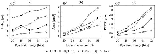
Figure 4.
Complexity characteristics of RNS comparators for Class 1 moduli sets.
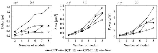
Figure 5.
Complexity characteristics of RNS comparators for Class 2 moduli sets.
Moreover, the speed advantage of the new comparators was achieved using less hardware resources, with only two exceptions. For large dynamic ranges, hardware reduction is significant, as it can exceed 40% compared to the least complex existing designs. For all cases considered, the SQT-based method of [25] consumes more hardware resources than any other method. Hardware complexity of the basic CRT-based comparator deserves some special comments, because most of it is the reverse converter, which is used anyway as a stand-alone circuit. Therefore, it should not be considered a contributor to the overall hardware complexity.
Finally, power-consumption seems the major advantage of the new comparators, as its reduction ranges from over 50% to over 178% for Class 1 moduli sets and from over 10% to over 130% for Class 2 moduli sets. Moreover, it was achieved using circuits which are faster for all cases considered. In this context, using specifically designed comparators instead of the CRT-based comparators (which actually require including the least amount of extra hardware: only the final comparator of a-bit numbers), could be of some practical interest. This is because once the reverse converter is activated just for the purpose of comparing numbers, it could be extremely power-consuming, as can be seen from the data listed in Table 5 and Table 8, as well as shown in Figure 4c and Figure 5c.
5. Conclusions
This paper proposes a new general approach to the comparison of the numbers represented in Residue Number System (RNS). It is based on a newly introduced concept of the modified diagonal function, which serves as a theoretical basis to develop a significantly faster and more efficient comparison algorithm. It made it possible to introduce a new positional characteristic of an RNS number which is strictly monotonic so that it makes it possible to precisely reflect a relative positioning of numbers. Now, unlike in existing algorithms, computations involving cumbersome operations of finding the remainder of the division by a large and awkward number are replaced with significantly simpler computations involving only a power of 2 modulus. The newly proposed comparator and its most efficient known counterparts applicable for arbitrary RNS moduli sets, designed using various methods for several sample moduli sets, were synthesized for the 65 nm technology. Performance estimations obtained suggest that the new circuits enjoy delay reduction ranging from over 11% to over 75%, compared to the fastest circuits designed using existing methods. Moreover, it is achieved using less hardware, the reduction can even reach over 41%, and accompanied by significantly reduced power-consumption which in several cases exceeds 100%. Therefore, it seems that the presented method leads to the design of what is currently the most efficient hardware comparators of numbers represented using a general RNS moduli set. The magnitude comparison of RNS numbers, besides being used directly (like in some implementations of recent cryptographic algorithms using RNS), is also essential for the implementation of other RNS non-modular operations like division, sign detection, and overflow detection. Future research will include extensions of the approach proposed to handle other difficult non-modular RNS operations like sign and overflow detection.
Author Contributions
Formal analysis, M.B., M.D. and S.J.P.; Funding acquisition, M.B. and M.D.; Investigation, M.B., M.D. and S.J.P.; Methodology, S.J.P. and A.T.; Project administration, M.B. and A.A.; Software, M.D. and P.P.; Supervision, N.C. and A.A.; Validation, M.B. and A.T.; Writing—Original draft, M.D., S.J.P. and A.T.; Writing—Review & editing, M.B., S.J.P. and A.T. All authors have read and agreed to the published version of the manuscript.
Funding
The reported study was funded by RFBR, project number 20-37-70023 and project NCFU.
Conflicts of Interest
The authors declare no conflict of interest.
Abbreviations and Symbols
| CRT | Chinese Remainder Theorem |
| DR | Dynamic Range |
| MDF | Modified Diagonal Function |
| MOMA | Multi-Operand Modular Adder |
| MRC | Mixed Radix Conversion |
| RNS | Residue Number System |
| SQ | Sum of Quotients |
| SQT | Sum of Quotients Technique |
| the number of bits to represent M | |
| the number of bits to represent | |
| the number of bits to represent | |
| D(X) | the diagonal function |
| the modified diagonal function | |
| the multiplicative inverse of mod | |
| RNS moduli set | |
| n | the number of moduli |
| the number of bits of the fraction part | |
| the residue modulo (mod) | |
| RNS representation of an integer X |
References
- Szabo, N.; Tanaka, R. Residue Arithmetic and Its Applications to Computer Technology; McGraw Hill: New York, NY, USA, 1967. [Google Scholar]
- Mohan, P.V.A. Residue Number Systems; Birkhauser: Basel, Switzerland, 2016; ISBN 978-3-319-41383-9. [Google Scholar]
- Nannarelli, A.; Cardarilli, G.C.; Re, M. Power-delay tradeoffs in residue number system. In Proceedings of the 2003 International Symposium on Circuits and Systems, 2003, ISCAS ’03, Bangkok, Thailand, 25–28 May 2003; Volume 5, pp. V-413–V-416. [Google Scholar]
- Cardarilli, G.C.; Del Re, A.; Nannarelli, A.; Re, M. Low-power implementation of polyphase filters in Quadratic Residue Number System. In Proceedings of the 2004 IEEE International Symposium on Circuits and Systems (IEEE Cat. No.04CH37512), Vancouver, BC, Canada, 23–26 May 2004; p. II-725. [Google Scholar]
- Patronik, P.; Berezowski, K.; Piestrak, S.J.; Biernat, J.; Shrivastava, A. Fast and energy-efficient constant-coefficient FIR filters using residue number system. In Proceedings of the IEEE/ACM International Symposium on Low Power Electronics and Design, Fukuoka, Japan, 1–3 August 2011; pp. 385–390. [Google Scholar]
- Chervyakov, N.I.; Lyakhov, P.A.; Babenko, M.G. Digital filtering of images in a residue number system using finite-field wavelets. Autom. Control Comput. Sci. 2014, 48, 180–189. [Google Scholar] [CrossRef]
- Keller, T.; Liew, T.H. Lajos Hanzo Adaptive redundant residue number system coded multicarrier modulation. IEEE J. Sel. Areas Commun. 2000, 18, 2292–2301. [Google Scholar] [CrossRef]
- Posch, K.C.; Posch, R. Residue number systems: A key to parallelism in public key cryptography. In Proceedings of the Fourth IEEE Symposium on Parallel and Distributed Processing, Arlington, TX, USA, 1–4 December 1992; pp. 432–435. [Google Scholar]
- Albicocco, P.; Cardarilli, G.C.; Nannarelli, A.; Re, M. Twenty years of research on RNS for DSP: Lessons learned and future perspectives. In Proceedings of the 2014 International Symposium on Integrated Circuits (ISIC), Singapore, 10–12 December 2014; pp. 436–439. [Google Scholar]
- Chokshi, R.; Berezowski, K.S.; Shrivastava, A.; Piestrak, S.J. Exploiting residue number system for power-efficient digital signal processing in embedded processors. In Proceedings of the 2009 International Conference on Compilers, Architecture, and Synthesis for Embedded Systems—CASES ’09; ACM Press: New York, NY, USA, 2009; p. 19. [Google Scholar]
- Patronik, P.; Piestrak, S.J. Hardware/software approach to designing low-power RNS-enhanced arithmetic units. IEEE Trans. Circuits Syst. I Regul. Pap. 2017, 64, 1031–1039. [Google Scholar] [CrossRef]
- Chang, C.-H.; Molahosseini, A.S.; Zarandi, A.A.E.; Tay, T.F. Residue number systems: A paradigm to datapath optimization for low-power and high-performance digital signal processing applications. IEEE Circuits Syst. Mag. 2015, 15, 26–44. [Google Scholar] [CrossRef]
- Akushskii, I.J.; Burcev, V.M.; Pak, I.T. A new positional characteristic of non-positional codes and its application. In Coding Theory and the Optimization of Complex Systems; Nauka: Alma-Ata, Russia, 1977. [Google Scholar]
- Miller, D.D.; Altschul, R.E.; King, J.R.; Polky, J.N. Analysis of the residue class core function of Akushskii, Burcev, and Pak. In Residue Number System Arithmetic: Modern Applications in Digital Signal Processing; IEEE Press: New York, NY, USA, 1986; pp. 390–401. [Google Scholar]
- Lu, M.; Chiang, J.-S. A novel division algorithm for the residue number system. IEEE Trans. Comput. 1992, 41, 1026–1032. [Google Scholar] [CrossRef]
- Dimauro, G.; Impedovo, S.; Pirlo, G. A new technique for fast number comparison in the residue number system. IEEE Trans. Comput. 1993, 42, 608–612. [Google Scholar] [CrossRef]
- Wang, Y.; Song, X.; Aboulhamid, M. A new algorithm for RNS magnitude comparison based on New Chinese Remainder Theorem II. In Proceedings of the Proceedings Ninth Great Lakes Symposium on VLSI, Ypsilanti, MI, USA, 4–6 March 1999; pp. 362–365. [Google Scholar]
- Dimauro, G.; Impedovo, S.; Pirlo, G.; Salzo, A. RNS architectures for the implementation of the ‘diagonal function’. Inf. Process. Lett. 2000, 73, 189–198. [Google Scholar] [CrossRef]
- Sousa, L. Efficient method for magnitude comparison in RNS based on two pairs of conjugate moduli. In Proceedings of the 18th IEEE Symposium on Computer Arithmetic (ARITH’07), Montpellier, France, 25–27 June 2007; pp. 240–250. [Google Scholar]
- Bi, S.; Gross, W.J. The Mixed-Radix Chinese Remainder Theorem and Its Applications to Residue Comparison. IEEE Trans. Comput. 2008, 57, 1624–1632. [Google Scholar] [CrossRef]
- Pirlo, G.; Impedovo, D. A new class of monotone functions of the residue number system. Int. J. Math. Model. Methods Appl. Sci. 2013, 7, 803–809. [Google Scholar]
- Chervyakov, N.I.; Babenko, M.G.; Lyakhov, P.A.; Lavrinenko, I.N. An Approximate Method for Comparing Modular Numbers and its Application to the Division of Numbers in Residue Number Systems. Cybern. Syst. Anal. 2014, 50, 977–984. [Google Scholar] [CrossRef]
- Piestrak, S.J. A note on RNS architectures for the implementation of the diagonal function. Inf. Process. Lett. 2015, 115, 453–457. [Google Scholar] [CrossRef]
- Chervyakov, N.I.; Molahosseini, A.S.; Lyakhov, P.A.; Babenko, M.G.; Lavrinenko, I.N.; Lavrinenko, A.V. Comparison of modular numbers based on the Chinese remainder theorem with fractional values. Autom. Control Comput. Sci. 2015, 49, 354–365. [Google Scholar] [CrossRef]
- Sousa, L.; Martins, P. Sign Detection and Number Comparison on RNS 3-Moduli Sets {2n − 1, 2n + x, 2n + 1}. Circuits Syst. Signal Process. 2017, 36, 1224–1246. [Google Scholar] [CrossRef]
- Vu, T.V. Efficient Implementations of the Chinese Remainder Theorem for Sign Detection and Residue Decoding. IEEE Trans. Comput. 1985, C–34, 646–651. [Google Scholar] [CrossRef]
- Hung, C.Y.; Parhami, B. Error analysis of approximate Chinese-remainder-theorem decoding. IEEE Trans. Comput. 1995, 44, 1344–1348. [Google Scholar] [CrossRef]
- Akkal, M.; Siy, P. A new Mixed Radix Conversion algorithm MRC-II. J. Syst. Archit. 2007, 53, 577–586. [Google Scholar] [CrossRef]
- Hwang, K. Computer Arithmetic Principles, Architecture, and Design; Wiley: New York, NY, USA, 1979. [Google Scholar]
- Piestrak, S.J. Design of residue generators and multioperand modular adders using carry-save adders. IEEE Trans. Comput. 1994, 43, 68–77. [Google Scholar] [CrossRef]
- Piestrak, S.J. Design of high-speed residue-to-binary number system converter based on Chinese Remainder Theorem. In Proceedings of the 1994 IEEE International Conference on Computer Design: VLSI in Computers and Processors, Cambridge, MA, USA, 10–12 October 1994; pp. 508–511. [Google Scholar]
Publisher’s Note: MDPI stays neutral with regard to jurisdictional claims in published maps and institutional affiliations. |
© 2020 by the authors. Licensee MDPI, Basel, Switzerland. This article is an open access article distributed under the terms and conditions of the Creative Commons Attribution (CC BY) license (http://creativecommons.org/licenses/by/4.0/).