QRS Differentiation to Improve ECG Biometrics under Different Physical Scenarios Using Multilayer Perceptron

Abstract

Currently, machine learning techniques are successfully applied in biometrics and Electrocardiogram (ECG) biometrics specifically. However, not many works deal with different physiological states in the user, which can provide significant heart rate variations, being these a key matter when working with ECG biometrics. Techniques in machine learning simplify the feature extraction process, where sometimes it can be reduced to a fixed segmentation. The applied database includes visits taken in two different days and three different conditions (sitting down, standing up after exercise), which is not common in current public databases. These characteristics allow studying differences among users under different scenarios, which may affect the pattern in the acquired data. Multilayer Perceptron (MLP) is used as a classifier to form a baseline, as it has a simple structure that has provided good results in the state-of-the-art. This work studies its behavior in ECG verification by using QRS complexes, finding its best hyperparameter configuration through tuning. The final performance is calculated considering different visits for enrolling and verification. Differentiation in the QRS complexes is also tested, as it is already required for detection, proving that applying a simple first differentiation gives a good result in comparison to state-of-the-art similar works. Moreover, it also improves the computational cost by avoiding complex transformations and using only one type of signal. When applying different numbers of complexes, the best results are obtained when 100 and 187 complexes in enrolment, obtaining Equal Error Rates (EER) that range between 2.79–4.95% and 2.69–4.71%, respectively.

1. Introduction

In the last years, improvements in sensors have produced more affordable and faster biometric acquisition systems, with higher processing capabilities. Besides, evolution in mathematics has led to faster and more accurate pattern recognition algorithms, such as those covered in machine learning.

Electrocardiogram (ECG) biometrics is one of the biometric modalities that has been noticeably improved thanks to machine learning algorithms. This modality is based on the electrical activity in the heart related to time represented by ECGs. ECGs are measured with electrocardiographs through different parts and angles of the body, allowing them to obtain the signal from several perspectives. Its standard acquisition results in 12 different types of signals or leads that provide different information about the heart’s performance [1]. These signals get frequently classified in two types [2]:

• Limb leads: require four sensors, placed on the right arm, left arm, left leg, and right leg. The latter functions as a ground. Limb leads are also divided into two categories:

  –

  Standard bipolar leads (I, II, and III): measure the voltages between left arm-right arm, left leg-right arm, and left arm-left leg, respectively.

  –

  Augmented unipolar leads (aVR, aVL, and aVF): measure the relative voltages concerning the extremities, instead of using ground references. They allow us to observe the previous signals from different angles.

• Chest (precordial) leads (V1, V2, V3, V4, V5, and V6): are calculated considering ground as a reference and require of six sensors placed carefully on different parts of the chest.

Figure 1 represents the general sinus rhythm signal, formed by the P waveform followed by the QRS complex and the T waveform. The different waveforms provide information about how the different areas of the heart perform. P represents the depolarization of the atria. The QRS complex is a consequence of the depolarization of the ventricles, and the T wave shows their repolarization [3].

ECGs can be used as a biometric signal because they are universal, unique, invariant enough with respect to its template and quantitative [5]. Every alive person can provide an ECG and it can be measured with commercial electrocardiographs. This biological signal also depends heavily on the morphology of the heart, which is unique even among healthy individuals. The addition of variations due to physiological conditions related to skin properties, gender, or age, makes ECGs unique for every person [6]. They are also considered stable in the long term and provide good data separation between genuine users and imposters [7]. To our knowledge, the first approaches using ECG signals for human identification were released in 2001 [8,9].

These types of signals are interesting for biometrics because of their nature. They are difficult to access without the user’s cooperation and susceptible to the specific scenario the user is in, due to variations such as those caused by heart rate o amplitude changes. These characteristics make them difficult to counterfeit while providing them with a lot of potential in biometrics.

The present work provides a study of the potential of Multilayer Perceptron (MLP) Neural Network structure for ECG biometric verification, extending the achieved results in Reference [10]. Achieving good performances with a classifier such as MLP results in relevant information, due to the challenging properties of the applied database. In addition, the feature extraction process is simplified by re-using the calculated data in segmentation, reducing it to a simple window selection. This simplification allows us to reduce computational processing time and cost. Finally, we provide the optimal configuration for the classifier, including the type of features and data size, as well as a discussion about the information these results provide about the dataset.

Related Work

Many different steps take part in a biometric system: the sensor should be comfortable to use and provide a good quality signal. The pre-processing needs to improve the signal quality to facilitate further feature extraction and requires to be done wisely, to avoid dealing with non-relevant data. Pre-processing aims to avoid slowdowns and lower performances in the final stage, where the classification takes place. The chosen algorithm must generalize properly with new data while only using limited available data. If one of these steps is performed poorly, it can affect noticeably to the system’s performance.

Out of the different steps, signal acquisition is probably one of the most problematic in ECG biometrics. Commercial sensors are developed for medical use, that is, electrocardiographs, providing good quality signals but they are not realistic to use in a biometric environment. Biometrics require easy-to-use sensors, as they contribute to a faster recognition process as users usually do not have previous knowledge. Besides, medical sensors are inconvenient due to sensor placing, which is time-consuming. Moreover, depending on the required lead, the sensors have more uncomfortable and complicated placing, such as those in the chest. Some portable ECG acquisition devices are available for the public, such as AliveCor’s KardiaMobile [11] and Nymi’s band [12]. They are focused on the type I lead as they only require the arms to be involved. The first is focused on health; the latter is the only one, to our knowledge, that uses ECG for recognition purposes. However, neither of them allows us to obtain raw samples. This fact limits the development of biometric systems with reliable and user-friendly sensors. However, working with medical sensors is common to set a baseline. It allows us to start from the most ideal case, due to the precision these devices provide and work towards more complex scenarios. As an alternative, other researchers develop their prototypes, adding more challenges in the system’s implementation [13,14,15].

Even if sensors collect signals with high signal to noise ratio (SNR), data needs to be prepared accordingly to facilitate the feature extraction process. The noise in ECGs usually comes from three main sources: baseline wanders and drift, power-line interference and muscle artifacts [16]. Baseline wander is usually in the 0.2–0.5 Hz range and power-line interferences are found from 50–60 Hz, so both can be removed with a band-pass filter [17]. The simultaneous removal of both types of noise is also achieved with alternatives such as Discrete Cosine Transform (DCT) [18] and Discrete Wavelet Transform (DWT), which allows decomposing the signal, however, it is not as frequent as band-pass filters [19]. In recent years, deep learning techniques such as Convolutional Neural Networks (CNN) have also been applied to this problem [20]. Muscle artifacts also provide high-frequency noise around 100 Hz and can get removed with a low-pass filter, but techniques such as Moving Average (MA) filters are also applied [21].

Fiducial point detection is usually the next step to filtering. These points are those such as the ones that take part in the sinus rhythm wave in Figure 1, but not limited to the ones represented. They behave as reference points to help in the following feature extraction process. The fiducial points to detect depending on the selected feature extraction approach. Some works only need to spot the QRS complex, and most of them apply the Pan-Tompkins algorithm [22] or modify it slightly [13]. Once the reference points are calculated, signals can be segmented accordingly if needed. It is common to select fixed ranges using the detected points as a reference [23].

The signal conditioning usually leads to the feature detection process. Literature divides this process into two main approaches—fiducial features, which are based on time and amplitude related metrics; and non-fiducial features, based on the shape of the whole signal or selected segments. The use of fiducial features is not a trivial task to achieve, because their accuracy relies on the performance of the fiducial point detection algorithm [24]. Non-fiducial features usually apply Fourier or Wavelet transforms [25,26]. Fiducial features tend to work better in databases with lower variability (i.e., databases with a low number of subjects), because it avoids the use of unnecessary data, deleting noise as the selected signal characteristics belong to specific, narrower regions. However, in databases with higher variability, non-fiducial features work better. They deal more efficiently with the higher chances of noise in a greater number of samples [27].

One of the most common techniques for ECG classification used to be Support Vector Machines (SVMs) [28] and the k-Nearest Neighbour classifier (k-NN) [7]. Although they are still applied techniques, Artificial Neural Networks (ANNs) have increased their popularity since they starting being used at the beginning of the last decade [29]. Concerning this, future approaches are expected to use ANNs and Deep Neural Networks, due to their potential to solve SVM and k-NN problems, while even improving the results of more conventional classifiers [19].

2. Materials and Methods

2.1. System’s Description

The system in this work follows a common approach in biometrics. The raw signal, in this case, ECG, goes through a pre-processing stage that improves the quality of the information. The data can go through transformations or detection algorithms for relevant reference points. After preparing the data, the feature extraction segments the most important information to go through the final classification.

2.1.1. Pre-Processing and Feature Extraction

The acquired ECG data follows the scheme in Figure 2. As referenced in Reference [10], to delete noise, the ECG signals pass through a fifth-grade Butterworth bandpass filter from 1 to 35 Hz. Once the signal is filtered; the goal is detecting the R peaks to help in further signal segmentation. The filtered signal gets differentiated, obtaining first and second differentiations, called Non-Differentiation (ND), First Differentiation (FD), and Second Differentiation (SD) respectively. FD and SD help in the R peak detection because they provide information about changes in ND. R peaks are the local maxima in ND and translate into local minima in FD. These local minima are easier to detect than the original R peaks because they are more prominent. In the case there are outliers, two adjacent segments get compared by correlation. SD finally helps to check that the final segments have the corresponding shape.

After the R peak references are calculated, the feature extraction consists of segmenting the QRS complex in ND, FD, and SD independently, obtaining 3 different types of signals, as seen in Figure 2. The segmentation is given by two variables: rng1 determines the number of signal points to the left of the reference point and rng2 the samples to the right including the reference point itself. This implies that the segments have a length of $rng1+rng2$ points, which are the selected feature points. N peaks specifies the number of peaks selected to form the matrix, selected by appearing order, which is the samples.

2.1.2. Classification

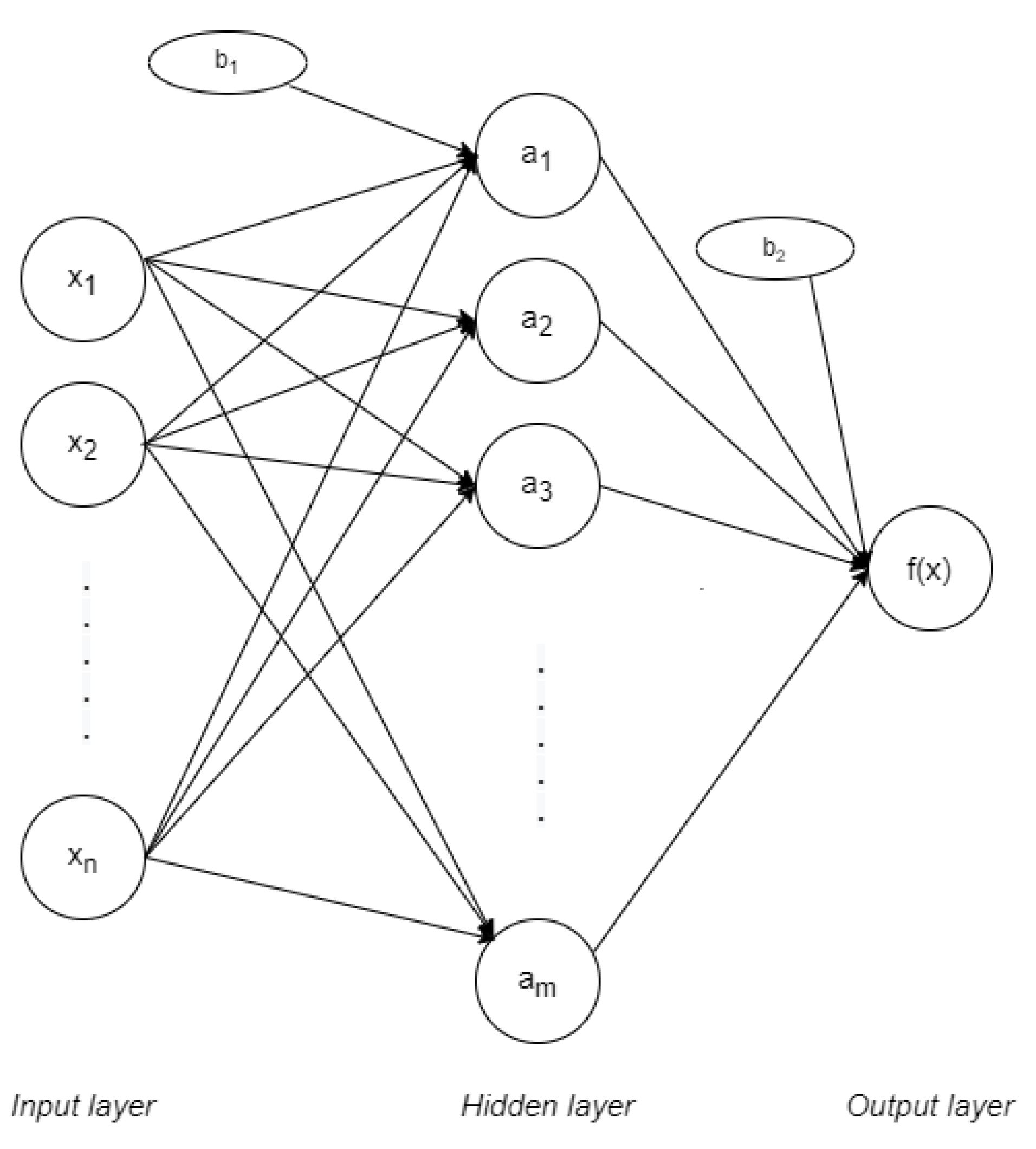
The chosen algorithm for classification is the MLP neural network. These structures have already been used as a classifier in ECG biometrics, achieving good performances [29,30]. Despite of the simplicity of this artificial neural network, it is considered a promising algorithm in the context of ECG biometrics [31]. MLP networks are applied in supervised learning and they have three main parts: input, output, and hidden layers, as represented in Figure 3. The input layer is formed by nodes or neurons that represent the different input features $\left\{x_i\right|x_1,x_2,\dots ,x_n\}$. Every feature is labelled with its correspondent class, $\left\{y_i\right|y_1,y_2,\dots ,y_n\}$. In the case of only having one hidden layer, the output layer gives the function in Equation (1) [32]:

$$f\left(x\right)=W_{2}g(W_1^{T}x+b_1)+b_2.$$

(1)

Where $W_1$ represents the sets of weights applied to every feature in the input layer. These weights vary between them, in the way that every feature $x_i$ has m different weights: one per node in the following hidden layer. On the same way, $W_2$ represents the weights applied in the hidden layer, at nodes $\left\{a_j\right|a_1,a_2,\dots ,a_m\}$. Value $b_1$ is the bias in the hidden layer while $b_2$ is the bias on the output layer. The activation function is represented by $g(·)$. The most common functions are identity (or no activation function), logistic, hyperbolic tangent (tanh) and rectified linear unit function (ReLU). All the corresponding functions are represented in

Table 1. Most common activation functions.

Name	Identity	Logistic	Tanh	ReLU
Formula	$g\left(x\right)=x$	$g\left(x\right)=\frac{1}{1+e^{-x}}$	$g\left(x\right)=tanhx$	$g\left(x\right)=max(0,x)$

.

As this structure works for supervised learning, the weights need to change in every connection after the data is processed to decrease the processed error. In this case, it is done by backpropagation, which comes from the Least Mean Squares (LMS) algorithm. These weights can be updated differently, depending on the approach for their optimization. The most common solver is of Stochastic Gradient Descent (SGD). Its formula depends on a factor called learning rate, which ensures the weights converge quickly.

2.2. Algorithm Modelling

As referred to in the previous section, the feature extraction depends on several values that need to be fixed for segmentation. The amount of data to introduce to the MLP classifier is determined based on these parameters, which rely on the database characteristics. At the same time, the MLP classifier depends on other parameters, called model hyperparameters, which vary depending on the implementation. Their values are set through a process called tuning, whose goal is achieving the most suitable values for correct classification.

2.2.1. Database

As ECG signals provide sensible information, releasing databases to the public is complicated due to privacy policies, leaving only a few databases to work with. Several databases are public in Physionet [33] being MIT-BIH Normal Sinus Rhythm (MIT-BIH NSR) and PTB [34] the most common ones in the literature. However, none of them are thought for human recognition but for helping in pathology classification, thus the acquisitions are done with commercial electrocardiographs. These databases provide long signals that are minutes or even hours long, while having the user in limited physiological conditions, usually resting. The ECG-ID database [35] is the only public one that aims for human recognition, providing 20-s signals. They are acquired by wrist electrodes and under two different conditions: sitting and free movement, making ECG-ID the closest to a biometric scenario.

According to ISO 19795 [36], data collection needs to be representative of the target application. This is the reason why in this case we need to consider that heart rates fluctuate constantly under different situations like stress and exercise. This parameter can be controlled in enrolment by helping the subject to relax. However, that is not something doable in recognition, where the subject must be independent. Adding this extra step would make the system less user-friendly and inconvenient. With these considerations, the previous databases focused on medical purposes do not provide the required data for biometrics. These databases tend to have long acquisitions and/or do not usually provide visits under different scenarios and/or days. In the case of ECG-ID, the free movement scenario is not specific enough about the activity, so the heart rate increase is not pursued, not making it useful for the study under more specific physiological conditions.

In terms of the capture device, working with professional medical sensors provides higher signal quality. This approach is chosen to remove as much noise as possible, maximizing the isolation of the signal behavior, even if it does not have the required usability for biometrics. The database acquisition is done using a Biopac MP150 system with a 1000 Hz sample frequency, as described in Reference [10]. The sensors obtain Type I lead, which is convenient in biometrics because it only involves the arms, measuring the voltage difference between left and right. Moreover, the placement of the limb sensors requires little expertise so their placement is similar between the different visits, in the pursuit of reducing this type of noise. The present work uses the second part of the extended database, as it is the only one that provides different physiological states. The collection is done with 55 healthy subjects in 2 different days, with two visits per day distributed as shown in

Table 2. Selected database visit distribution. The four visits are re-named as shown, based on the type of scenario: R1 and R2 for resting while sitting down, S for resting while standing up, and Ex for exercise.

Day 1		Day 2
Visit 1 (R1)	Visit 2 (S)	Visit 1 (R2)	Visit 2 (Ex)
Resting, sitting down	Resting, standing	Resting, sitting down	After exercise (average 130 bpm)

. Each visit records 5 signals of 70 s duration per signal with a 15 s posture adjustment between every recoding.

The applied database remains private, due to the General Data Protection Regulation (GDPR) by the European Government. The law started its implementation in 2018 and considers that biometric data is sensitive. The GDPR takes into consideration the potential need to use this data in research but demanding some specific conditions. As this database was collected before the GDPR implementation, it does not fulfill the legal criteria to get published.

2.2.2. Implementation

Classification

The classifier implementation is done using Python 3 and using scikit-learn [37]. Every user provides 5 signals per visit, from which ND, FD, and SD are calculated. The first and last 5 s are discarded from every signal, obtaining a 60 s signal. From every one of them, 50 R peaks are detected and segmented accordingly to extract the QRS complex. The complex has the R peak on the 101th position and is formed by 200 points. All complexes get concatenated, summarizing the database into three types of matrixes for every visit: one per type of signal differentiation. Train and test sets are extracted from this data, selecting the differentiation and visit differently based on the type of experiment to carry out. The training matrix, $X_{train}$, has dimensions $[r_{train}\times c]$ where c is the number of columns or points in the QRS complex and $r_{t}rain$ is the number of rows, which corresponds to the number selected complexes. Similarly, testing data, $X_{test}$, has $[r_{test}\times c]$ dimensions.

Some of the required hyperparameters for the MLP classifier need to be set to a specific value due to previous knowledge and considerations. Fixing some of the hyperparameters make the hyperparameter tuning easier. The number of hidden layers is set to one because it usually achieves proper results and avoids extra slowdown [38]. Regarding the type of solvers, not only SGD is an option, but also another SGD-based optimizer, adam [39], and L-BFGS, which is a quasi-Newton optimizer. However, among these three solvers, only adam is used due to our preliminary results where SGD and L-BFGS provide very low-performance results. This decision discards the option of applying a specific learning rate formula because it is only applied to SGD solvers. In this case, we only need the size of the step that updates the weights, which is fixed to the default value, 0.0001. Convergence is assumed when the result does not improve significantly in a specific number of iterations, and this hyperparameter is also given by its default value which is 10.

Table 3. Summarization of the fixed MLP hyperparameters.

Hyperparameter	Description	Value
Hidden layers	Number of hidden layers.	1
Solver	Function used for weight updating.	adam
Learning rate	Function used to update the learning rate that takes part in the solver.	Not applicable with adam solver.
Learning rate step	Step size for the learning rate updates.	0.0001
No change iterations	Number of iterations with no relevant change to consider convergence.	10

summarizes the given values to the discussed parameters and their functionality.

After fixing the previous values, the remaining hyperparameters need to be fixed to reach an optimal system’s performance. Even though there is one hidden layer, the number of nodes in the hidden layer needs to be assessed. The same happens with the activation function which can be any of those in Table 1. This implementation solver optimizes the loss function in Equation (2). This formula has two components: the first summation corresponds to Cross-Entropy, where t indicates whether a class is positive or not, $p\left(s\right)$ is the softmax output implemented by the library in a multiclass case and C is the number of classes; the latter belongs to L2-regularization, where $\alpha$ or alpha is the penalty term and ${\left|\right|W\left|\right|}_2$ represent the Euclidean norm of the weight hyperparameters. The value alpha avoids underfitting when it gets a positive value lower than 1 and it needs to be specified.

$$Loss(W;t,p\left(s\right))=-\sum _i^C{t}_{i}log(p{(s)}_i)+{\alpha \left|\right|W\left|\right|}_2^2.$$

(2)

Finally, closely related to the convergence assumption, is the tolerance hyperparameter. The tolerance provides the quantity the loss function needs to be improved to keep iterating.

Performance Measurement

To evaluate the performance of a verification system, the ISO 19795 [36] does not encourage the use of single values such as percentages, because they miss relevant information. The Detection Error Trade-off (DET) graphs are the main tool instead, as they show the False Non-Match Rate (FNMR) and False Match Rate (FMR) evolution with respect to different thresholds. The point where both are equal represents the lower possible error rate and is called the Equal Error Rate (EER) [5].

The decision on whether the user is whom he/she says is based on the scores retrieved by the classifier. This implies that depending on the applied criteria, the system could not verify genuine users (FNMR) when doing otherwise with impostors (FMR). Some biometric applications, such as the entrance of a gym, would rather have higher FMR as a trade-off for a fast authentication process. On the other hand, if the authentication is for a bank account, the system would rather have high FNMR. This could increase the probability of asking the user for their data more than once, making the process more inconvenient. The trade-off between convenience and security must be determined in design, depending on the system’s target application.

In the case of the selected database, classes for the test samples are known. With this information, the model’s performance can be assessed from the probabilities retrieved by the MLP classifier. Typically, scorers or loss functions are applied for this purpose. However, in this case, we implement a different approach and apply a custom function that implements the EER calculation.

To do so, when several samples from the same class are used in the test set, all the probabilities are unified applying the mean. This provides only one probability vector for that given class in the test, containing the mean probability for every comparison combination. By paying attention to the reference class in every comparison, we can divide these results into two types: mated that is, when reference and comparison classes are the same; and non-mated if otherwise. From them, we can obtain the False FNMR and FMR. As they represent both possible types of error, the crossing point of both lines gives the EER, acting as the score for further optimization.

Despite ISO guidelines, performance metrics are still heterogeneous in the state-of-the-art. To be able to compare this work’s results with similar ones in the literature, accuracy calculation was also implemented. In this case, a threshold is applied to the scores retrieved by the classifier, giving values 0 (if discarded) or 1 (if verified). The accuracy is calculated by doing a simple division of total correct classifications by the total number of samples.

2.2.3. Hyperparameter Tuning

The tuning process is done independently for ND, FD, and SD signals, to observe which one provides better performance results. The type of signal is not specified through this section, but it is repeated similarly for the three of them. The only difference is on the model hyperparameters and their performance results.

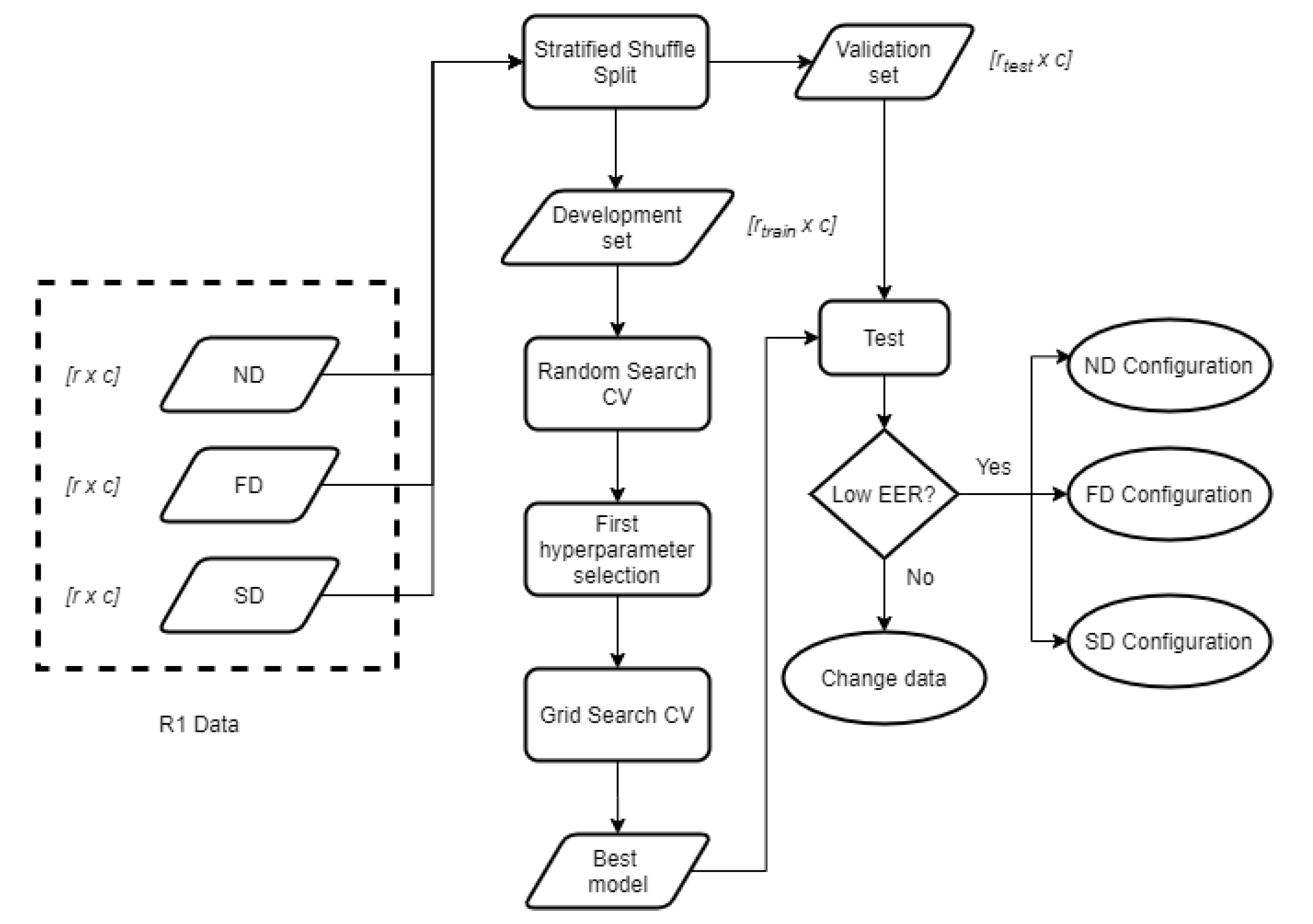
The goal of tuning is determining the most optimal set of values to model our data. This work achieves these results by first applying a Random Search, as it has been proven a suitable technique that requires less computational time [40]. The exhaustive Grid Search is performed afterward, as represented in Figure 4. The whole tuning process is done based on the data in one of the visits, which behaves as the enrolment. In this case, it is the data in R1, which is expected to be the most stable set because the user’s relaxed and sitting down. This process is repeated individually for ND, FD, and SD, obtaining 3 different configurations, one per signal.

As for testing the model after the tuning process, the test data needs to be new, we need to split R1 into two parts: one is used for training (development matrix), and the other one for validating (validation matrix) the trained models. We decided to set the train size to 50% to obtain the same sizes for training and validating, which results in 125 QRS complexes per user in both matrixes.

The division is done using a method called Stratified Shuffle Split, which selects the samples randomly but keeping the class proportion to avoid having an unbalanced model. The random shuffling is replicable, so results are not biased by different shuffling orders.

Random Search

The Random Search method sets a number of random hyperparameter combinations, training a new model for each one of them. The activation function can be all four types in Table 1. The rest of the hyperparameters are numerical, and the selected range of values tries to represent extreme values, with equidistant middle values to observe if performances are correlated to little changes in any of them, as seen in

Table 4. Possible values for the remaining hyperparameters.

Hyperparameter	Possible Values
Hidden layer size	1, 25, 50, 75, 100, 125, 150, 175, 200, 225, 250
Activation	Identity, logistic, tanh, ReLU
Alpha	0.0001, 0.0005, 0.001, 0.005, 0.01, 0.05, 0.1, 0.5
Tolerance	0.01, 0.05, 0.1, 0.5

. Tolerance is still relatively low to try to achieve more accurate results.

In this case, we obtain 50 random value combinations by training with the development set. The MLP training is done using cross-validation to observe how well the model performs under different train and test sets. In this case, the cross-validation process is done 5 times, dividing the development set into 80% training and 20% test. This division is also done by using Stratified Shuffle Split. The final performance results for every combination contains the mean EER through all the splits.

Table 5. Best hyperparameter values in Random Search and their Equal Error Rates (EERs) for Non-Differentiation (ND), First Differentiation (FD), and Second Differentiation (SD).

Signal	Hidden Layer Size	Activation	Alpha	Tolerance	Mean EER (%)
ND	200	logistic	0.01	0.05	0.13
	100	logistic	0.01	0.05	0.23
	125	logistic	0.1	0.01	0.50
FD	200	identity	0.001	0.05	0.16
	200	relu	0.0005	0.05	1.27
	75	logistic	0.0001	0.01	1.54
SD	150	tanh	0.0001	0.01	0.95
	125	identity	0.0001	0.01	1.28
	175	tanh	0.005	0.01	4.59

shows the best 3 results for ND, FD, and SD in descending order.

Grid Search

Selecting only the present values in Table 5, Grid Search performs training similarly to Random Search, but doing it exhaustively that is, doing it for every possible combination of hyperparameter values instead of for a limited number. This can be done due to the value reduction Random Grid has provided, because it allows us to discard a huge range of potentially bad combinations, decreasing the processing time significantly. The results are summarized in

Table 6. Best hyperparameter values in Grid Search and their EERs for ND, FD and SD.

Signal	Hidden Layer Size	Activation	Alpha	Tolerance	Mean EER (%)
ND	200	logistic	0.01	0.05	0.13
FD	200	identity	0.001	0.05	0.16
SD	150	tanh	0.0001	0.01	0.95

. This combination gets tested with the validation data, to confirm it performs properly under new data.

3. Results

By only using half of the R1 data for training, we observe that best verification performances are obtained through ND signals, followed by FD and SD. However, this does not imply that is going to happen when applying different train and test sets. The tuning has allowed us to fix those hyperparameters, ensuring the result will be as good as it can get when using data in R1 as training and testing. However, we need to check if the selected structures for ND, FD, and SD behave correctly in other cases.

The different combinations of the train and test sets provide different information. Good performances using the same visit for training and testing means that the applied data has low intra-class variability and high inter-class variability. This translates into the same user signals being similar enough among them, but also significantly different from the rest of the users. When using different visits in training and testing, we can observe how intra-class and inter-class variabilities are affected. Once the most suitable training set and type of signal are determined, we vary the amount of training data to observe changes in the final performance.

3.1. Results within the Same Visit

For every type of signal and visit, 50% of the data is used for training and testing is carried out with the remaining information in the visit. The random sample selection is the same in ND, FD, and SD. This process gives an idea of how the system configuration works within different user visits. In

Table 7. EER (%) results for every type of signal under the same visit.

	R1	S	R2	Ex
ND	0.10	0.13	0	0.17
FD	0	0	0	0.07
SD	0.20	0	0.20	0.77

we can see that results are 0 or close enough to 0. As expected, the highest values are calculated under Ex, due to its higher variability. FD is the one with the lowest EER values. SD provides good results under S but performs poorly in the remaining visits.

Figure 5 represents DET graphs for ND, FD, and SD when using Ex in training as an example. As seen in the previous results, FD has the best performance, followed by ND and SD. In the three types of signal, the FNMR reaches higher percentages than the FMR, meaning that false negatives are more common than false positives. In a biometric environment, this could lead to the need of repeating the recognition process even if the user is whom they say to be.

3.2. Results within Different Visits

In the previous experiment, both enrolment and recognition data were acquired under the same scenario. Nonetheless, to represent the potential signal variation in a biometric environment, we need to study the results when using different visits for enrolment and recognition. The scheme in Figure 6 represents the steps followed to obtain the different results when using R1 as a train set or enrolment and the remaining visits as a test set or recognition data. It considers a variable training size that refers to the data proportion that is going to be used for training. In the case it is lower than 1, that is, not all the samples are used, we use Stratified Shuffle Split for the division. The variable xD represents the different types of signals, where x can be changed to refer to ND, FD, or SD. This scheme is followed also by using the remaining visits S, R2, and Ex. Results for all 4 different train sets are represented and discussed in the following paragraphs. For comparison purposes among different graphs, the y-axis is fixed to be common in all of them.

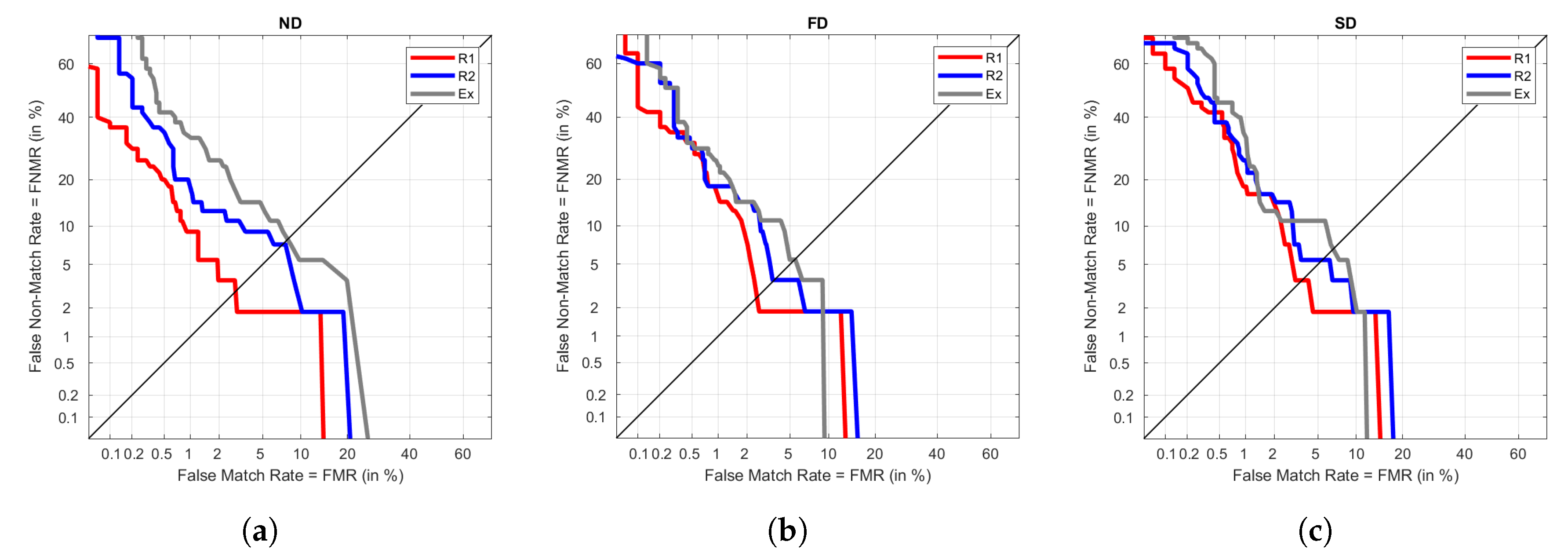
Figure 7 represents all the DET performance curves when R1 is used as the enrolment or train set. The best performance for S is achieved under ND. However, it also provides the worst results of Ex. We can also observe that the results of the three visits are more spread in ND, obtaining very different results depending on the visit. In the cases of FD and SD, the results are more similar among visits, being better in the case of FD as it provides lower FNMR and FMR throughout the graph than SD.

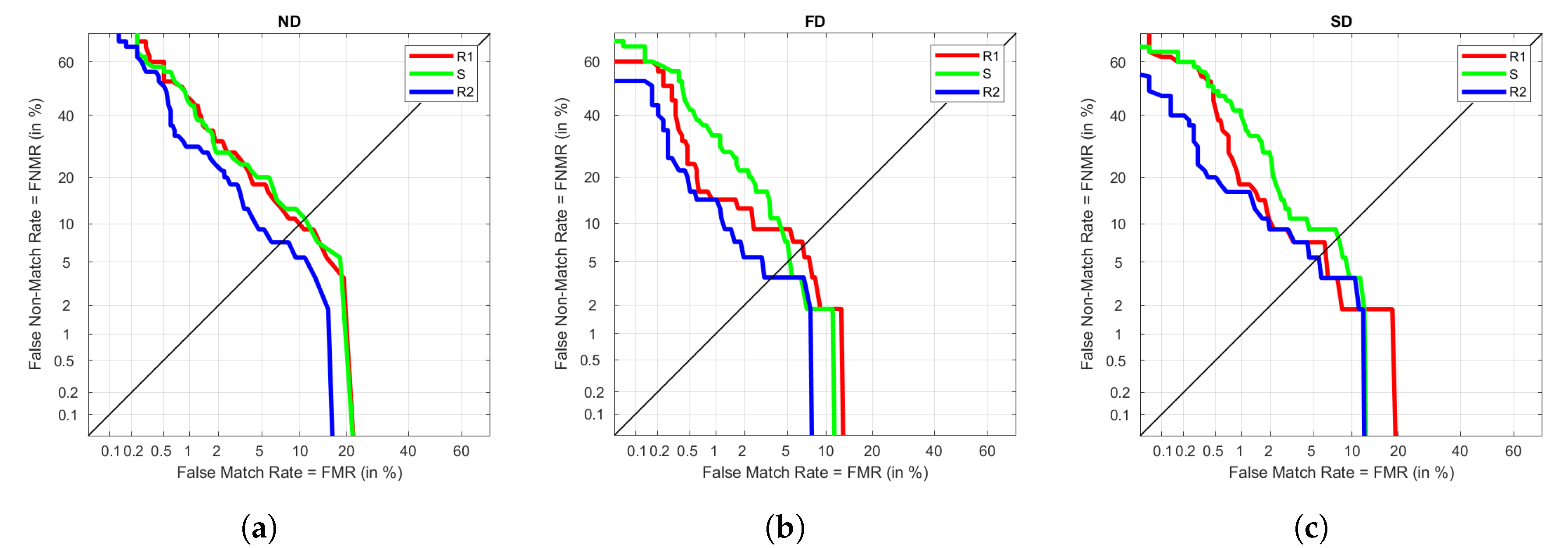
Similarly, Figure 8 represents DETs for S as training. We observe the same pattern as before, where ND provides more differentiated results among visits, whereas FD and SD have similar trends. The best result is always achieved under R1, which tells that the train and test visits are not highly differentiated. It could be due to the influence of being taken on the same day, or a not relevant variation in the data between sitting and standing. The results for Ex and R2 are not significantly different either because they keep a low EER.

In the case of R2 in training, ND keeps performing worse than FD and SD, as seen in Figure 9. However, generally, the three signals have similar performances but reach the best ones under FD, although the improvement is not very noticeable. In these graphs we observe Ex reaching values like those in R1 and S as training, which would not happen in the previous cases. This shows that even R2 and Ex are were taken under different heart rates in the users, the fact that they were close in time results in good performances, obtaining EER around 5%.

Finally, Ex is used as training, collecting its results in Figure 10. As expected, due to the higher heart rate in this visit, results do not improve the ones seen so far. However, it is consistent with FD being the best signal in performance. In addition, results for R2 are the lowest ones, reinforcing the theory that the signal taken in the same day behaves well, despite the different heart rate. Again, R1 and S have similar trends.

When using the same data set in training and testing, we observed that FD achieved better results, and it has been consistent when testing with different visits. Even though best results are obtained with R1 as train set, keeping the EER around 5% or lower when using FD, we have observed that similar results have also been obtained using FD when R2 is the train set. This provides two important pieces of information: resting is the most suitable condition for the user to be enrolled with, and the system still provides good results when identifying with information taken on different days.

Final Configuration and Its Results

Considering all the previous processes and results, the final MLP configuration is summarized in

Table 8. Final MLP configuration.

Number of hidden layers	1
Hidden layer size	200
Activation	Identity
Alpha	0.001
Tolerance	0.05
Solver	Adam
Learning rate step	0.0001
No change iterations	10

, considering the previously fixed hyperparameters in Table 3. The enrolment data must be acquired in a relaxed state while relaxing, providing 125 QRS complexes. To reduce the computational cost, the only type of signal fed into the classifier is FD, as it has shown to result in a good performance on its own. Under this configuration, the EER is calculated when using 125 complexes of FD data in R1 to enrol. It results in 3.64%, 3%, and 5.54% for S, R2, and Ex visits, respectively.

3.3. Results for Different Enrolment Sizes

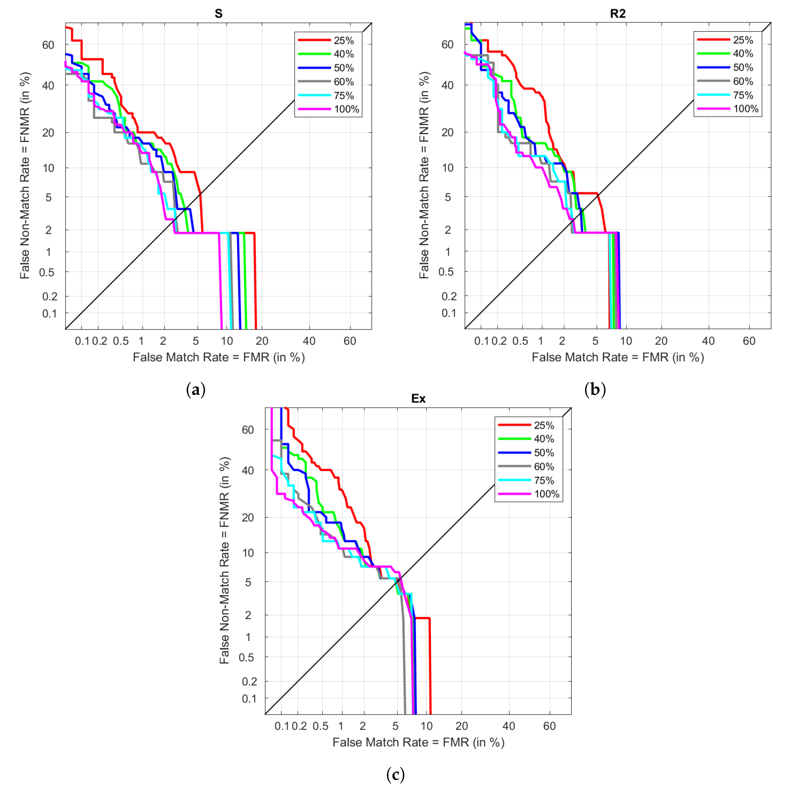
The determination of the most optimal MLP configuration was done using only one of the visits. It was required to split the data between training and validation, using only half of the available data for modeling. Using the highest amount of possible data could lead to better results. However, providing too much information could cause overfitting, resulting in a model that is not capable of generalizing properly with new samples. The previous section already set the most suitable configuration when using 50% of R1 data with FD. The goal of this experiment is to vary the training proportion to observe how the initial results get affected. The training is done using 25%, 40%, 50%, 75%, and 100% of the available R1 FD data, while the testing is the same as the one in the results between different visits. This data is plot in Figure 11. The different performances under S are plot in Figure 11a. The lowest EER is obtained when using 100% of the available data in training, increasing as the proportion decreases. However, we can see that there are not huge differences between using 60% or 75% of the data, as it also happens with 40% and 50%. However, when data is reduced to only 25%, the EER almost doubles the previous result. Similarly, Figure 11b represents these results in the case of R2. In this visit, using 100% provides closer results to those in 80 and 75%. As seen in the case of S, 40% and 50% do not provide significant differences, and decreasing the enrol data to 25% provides the same impact as before. In the case of Ex, represented in Figure 11c, results do not change significantly between sizes. Even though we observe 100% as the higher in EER, given that all results are close to each other, this subtle difference could have nothing to do with the training size.

All the EER results are collected in

Table 9. EER (%) for different enrolment proportions when using R1 FD for enrolment.

	Visit	S	R2	Ex
Enrol Proportion
25%		5.42	3.64	5.05
40%		3.64	2.79	4.95
50%		3.64	3.00	5.45
60%		2.73	2.46	5.42
75%		2.69	2.09	4.71
100%		2.02	1.88	5.52

. As seen graphically, using only 40% of the available data for enrolment provides similar results to those in 50%, being even slightly improved. This change could mean going from 125 necessary cycles to 100, decreasing the enrolment data acquisition in a few seconds. Increasing to 60% also makes a slight improvement, although not in the case of Ex. Using 75% of the data results in the lowest EER for Ex and one of the lowest for S and R2, being under those obtained in 100%. However, the different EER results when increasing the proportion from 75% to 100% is noticeable, as S and R2 perform better by causing a poorer performance in Ex. This is one of the reasons to avoid using such a long enrolment if there are chances of having very different heart rates in recognition.

After analysing these results, we can say that our system can reach results between 2.79% to 4.95% EER, using 100 QRS complexes. If the purpose of the system requires higher performances with the expense of longer enrolments, increasing the size of the data set is a good approach. Providing 187 QRS complexes for enrolment provides an EER between 2.69% and 4.71%. Finally, results in terms of accuracy are represented in

Table 10. Accuracy (%) for different enrolment proportions when using R1 FD for enrolment.

	Visit	S	R2	Ex
Enrol Proportion
25%		97.48	97.55	97.48
40%		97.82	97.89	97.78
50%		97.98	98.05	97.78
60%		98.11	98.17	98.04
75%		98.26	98.35	98.15
100%		98.40	98.49	98.26

applying a threshold of 0.5. The achieved accuracy under every condition is higher than 97% considering single heartbeats. We can also observe that the accuracy increases slightly up to 1% when increasing the training data.

3.4. Results Comparison

There are heterogeneous techniques throughout literature along with all different steps in the process. Not only results but also tools need to be taken into consideration. The selected works to compare our results to, are chosen due to similarities with the present work, as well as being relatively recent, going from 2017 to 2019. The techniques and some of their results are summarized in

Table 11. Summary of results and tools from state-of-the-art with similar characteristics.

Reference	Database	Users	Features	Classifier	Result
[15]	Private	18	Heartbeats	MLP	Accuracy: 89%
[31]	ECG-ID	90	Heartbeats	MLP LDA	Accuracy: 84–89.3% Accuracy: 93.28%
[10]	Proposed database (extended)	104	SWT for heartbeats	LDA	EER: 1.74–5.47%
Proposed work	Proposed database (only users with exercise)	55	QRS complex	MLP	Short enrol: EER: 2.79–4.95% Accuracy: 97.78–97.89% Long enrol: EER: 2.69–4.71% Accuracy: 98.15–98.35%

.

The criteria to select these works were based on several facts: getting databases whose characteristics were the closest to the proposed one, while having similar segmentation processes and/or same classification algorithm. However, fulfilling all conditions at the same time of providing similar procedures in testing and metric calculations is very complicated. We have found that similar works usually implement the classification accuracy as performance measurement, instead of calculating DET graphs. In addition, due to different procedures and tools, having higher accuracies or lower EERs does not imply better performances, as conditions vary among all of them. There are even discrepancies when working with the proposed database, as the verification performance is obtained considering its extended version.

These drawbacks are also the reason to not test the proposed algorithm in public databases. This work deals with the problem of verification using ECG with significant heart rate variations, but there are no public databases with these characteristics. As most databases are focused on pathology detection, they include non-healthy subjects, colliding with the assumption of healthy sinus rhythm for the QRS segmentation. Moreover, the databases that collect information on healthy users do not provide heart rate changes to test our approach.

Nonetheless, our work provides good results in comparison to the work with the extended version of the database [10]. We need to emphasize that in the extended version, 49 out of 104 subjects provide the Day 1 scenario in both days, making the EERs not comparable. Obtained accuracies for the best solutions (40% and 75% of training data) are also good reaching up to 98.35%. The proposed classifier structure is a very simple ANN that only requires using differentiation in the segmented QRS, avoiding more complex transformations, and decreasing the computational cost, which is important to export algorithms to mobile devices. It also deals with a good number of users and considers different more physiological conditions that are not considered in the ECG-ID database.

4. Discussion

This work proposes a machine learning algorithm for ECG verification by avoiding extra calculations in the feature extraction process. This is achieved by re-using already calculated data in the segmentation process to train the model. Skipping these extra calculations reduces the complexity and time consumed by the system while using simple differentiated QRS complexes. The selected classification algorithm is the MLP neural network, which gets its optimal hyperparameter configuration after a tuning process. To reach this goal, we applied a database which considers specific physical states and different acquisition days to obtain more information about the recognition. The tuning process and the following performance evaluation have provided a deep study in the behaviour of the different types of scenarios.

In addition, the optimal configuration provided an interesting result—the final activation function is identity, which corresponds to a linear function. This feature leads the system to be simplified to a linear system, which implies the possibility of being solved as linear regression. Even though more activations such as ReLU also achieved good results in tuning, finding out the results of this approach could lead to relevant information. Doing further research in this matter can provide information about how these data behave and if the selected features are representative enough, simplifying the classification.

Regarding the final MLP model, we have observed that the first differentiation in the QRS complex provides the best results. From these results, we can infer that how fast the waveform varies is a way to enhance the differences among users. In addition, we have seen how using different sizes of enrolment data affects the performance. The selection of this feature depends on the purposes of the biometric system, as some environments require shorter enrolment processes but do not mind lower performances, while others could choose otherwise. In conclusion, we have shown that using around 100 QRS complexes is good enough for the system, and it is not recommended to exceed 190 in enrolment unless it is known that the recognition data is controlled and heart rates are low enough. These configurations reach the best EER of 2.69% to 4.71% when applying the longest type of enrolment. Nonetheless, looking for more combinations of the signal differentiation could be a new way to improve performances.

The present work also focuses on the differences between three types of physiological situations for the user, due to a lack of public databases with these characteristics. The chosen database collects different visits in different scenarios, proving that MLP is capable of working properly under these conditions. The system also reduces the computational complexity and time with its simplicity. This matter is key for potential algorithm adaptation in mobile devices, setting a good precedent for further research on this issue.

Moreover, we have proven that as it can be expected, different heart rates between the enrolment and recognition data provide lower performance. In addition, even if the scenarios are different, the performance does not decrease as much if the data is taken on the same day. Having huge time differences between data acquisition in enrolment and recognition is unavoidable, so it is very important to have a controlled environment when acquiring enrolment data, being preferable to get it when the user is sitting down and relaxed.

Achieving these results allows us to do further research related to the different stages of a biometric system. Changing the sensor into a more usable one, such as a wearable, would likely provide a signal with lower quality, adding challenges in software. Doing an extension for the original database could also be an interesting approach: adding more types of scenarios such as stress; different physical conditions such as those given by age or exercise frequency or including acquisitions in hot or humid environments. Making ECG biometrics more inclusive with users with pathologies is also a pending task. This could be potentially achieved by avoiding the segmentation process with deep learning techniques.