Article

Comparison of Different Missing-Imputation Methods for MAIAC (Multiangle Implementation of Atmospheric Correction) AOD in Estimating Daily PM2.5 Levels

1
Department of Epidemiology and Preventive Medicine, School of Public Health and Preventive Medicine, Melbourne, VIC 3004, Australia
2
State Key Laboratory of Organ Failure Research, Department of Biostatistics, Guangdong Provincial Key Laboratory of Tropical Disease Research, School of Public Health, Southern Medical University, Guangzhou 510515, China
3
Department of Urban Planning and Design, The University of Hong Kong, Pokfulam, Hong Kong
4
State Key Laboratory of Information Engineering in Surveying, Mapping and Remote Sensing, Wuhan University, Wuhan 430079, China
5
Institute for Environmental and Climate Research, Jinan University, Guangzhou 511443, China
*
Author to whom correspondence should be addressed.
Remote Sens. 2020, 12(18), 3008; https://doi.org/10.3390/rs12183008
Submission received: 25 July 2020 / Revised: 3 September 2020 / Accepted: 14 September 2020 / Published: 15 September 2020

Abstract

:
The immense problem of missing satellite aerosol retrievals (Aerosol Optical Depth, (AOD)) detrimentally affects the prediction ability of ground-level PM2.5 concentrations and may lead to unavoidable biases. An appropriate missing-imputation method has not been well developed to date. This study developed a two-stage approach (AOD-imputation stage and PM2.5-prediction stage) to predict short-term PM2.5 exposure in mainland China from 2013–2018. At the AOD-imputation stage, geostatistical methods and machine learning (ML) algorithms were examined to interpolate 1 km satellite aerosol retrievals. At the PM2.5-prediction stage, the daily levels of PM2.5 were predicted at a resolution of 1 km, based on interpolated AOD and meteorological data. The statistical performances of the different interpolation methods were comprehensively compared at each stage. The original coverage of retrieved AOD was 15.46% on average. For the AOD-imputation stage, ML methods produced a higher coverage (98.64%) of AOD than geostatistical methods (21.43–87.31%). Among ML algorithms, random forest (RF) or extreme gradient boosted (XG-interpolated) AOD produced better interpolated quality (CV R2 = 0.89 and 0.85) than other algorithms (0.49–0.78), but XGBoost required only 15% of the computing time of RF. For the PM2.5 predicted stage, neither RF-AOD nor XG-AOD could guarantee higher accuracy in PM2.5 estimations (CV R2 = 0.88 (RF or XG-AOD) compared to 0.85 (original)), or more stable spatial and temporal extrapolation (spatial, (temporal) CV R2 = 0.83 (0.83), 0.82 (0.82), and 0.65 (0.61) for RF, XG, and original). For the AOD-imputation stage, the missing-filled efficiency depended more on external information, while the missing-filled accuracy relied more on model structure. For the PM2.5 predicted stage, efficient AOD interpolation (or the ability to eliminate the missing data) was a precondition for the stable spatial and temporal extrapolation, while the quality of interpolated AOD showed less significant improvements. It was found that XG-AOD is a better choice to estimate daily PM2.5 exposure in health assessments.

Graphical Abstract

1. Introduction

Since 1998, in China and India, industrialization, economic development, and a substantially increasing energy demand has led to over five times and triple growth in China’s and India’s coal-fired power, respectively [1]. Although accounting for 36% of the world’s population, they have accounted for 59% of global disease burden attributable to fine-particulate pollution [2]. Many previous epidemiological studies around the world have linked short-term PM2.5 exposure to emergency hospital admissions and even deaths from acute or chronic illnesses such as asthma and stoke [3,4,5,6,7]. Despite such severe air pollution conditions and widely publicized concerns, there are sparse PM monitoring stations, and this is a significant hurdle for assessing pollution exposure. Among the 7.5 billion people worldwide, only approximately 5.9 billion (approximately 80%) people live in regions that are covered by available PM readings [8]. This is because of the high cost of building and maintaining monitoring sites.
In recent years, there has been an increasing trend to use satellite aerosol optical depth (AOD) for estimating ground-level PM2.5 concentrations. Compared with conventional monitoring, the lower cost, higher coverage, and higher spatial resolution are advantageous, but the inherent drawbacks of AOD are obvious and difficult to solve. The most critical issue is the high missing rate of satellite-retrieved AOD, potentially related to orbit patterns, cloudiness, polar night, and surface reflectivity [9,10]. Kahn et al. [10] reported that the fairly low likelihood (approximately 15%) of successfully extracting aerosol retrievals from satellite instruments is a global problem, and the high missing rate of aerosol retrievals makes it impossible to estimate short-term PM2.5 exposure in continuous time series or most time in the research period [11,12,13]. Furthermore, some reported daily PM2.5 measurements have presented different distributions between AOD-missing days and other days [14]. Compared with long-term pollution exposure, short-term health assessments rely more on integral temporal variations in exposure. A drawback of satellite-based estimates is that they cannot represent the real distribution of PM2.5.
For addressing this issue, AOD retrievals need to be imputed before estimating PM2.5 levels where AOD is an important input variable. Multiple geostatistical approaches have attempted to impute AOD. Some examples are inverse distance weighting, nearest neighbors, kriging, generalized additive models or multiple imputation [15,16,17], but have achieved relatively low efficiency (missing rate after interpolation approximately 30–50%) and quality (cross-validation R-square approximately 0.34–0.64). We previously proposed [8] a two-step (TS) interpolation (first using data from Terra to estimate Aqua missing values, then inverse distance weighted interpolation (IDW) for second step) to reduce the AOD-missing rates from 87.91% to 13.83%, and maintain a relatively satisfactory performance (CV R-square = 0.76). However, the coverage needs to be increased further, and higher efficiency of interpolations were also required, especially when the sample size increased with a higher resolution in (Multiangle Implementation of Atmospheric Correction) MAIAC AOD (32 times with resolution from 3 km to 1 km). Moreover, our previous method [9] was over-dependent on geostatistical interpolation and ignored some influences of other external information such as meteorological data and cloud fraction on the temporal dimension, which inevitably weakened the efficiency and accuracy of imputation. This study endeavors to improve upon some weaknesses in the previous study. Machine learning methods can assist with solving these problems due to their strengths in capturing complex non-linear relationships and high dimension interactions [9,18]. We attempted to select an optimal method by comprehensively comparing a variety of machine learning algorithms and geostatistical approaches in imputing missing data of AOD.
After imputing missing data of AOD, we previously confirmed that the combined method of non-linear exposure-lag-response model (NELRM) and XGBoost is superior to other nine ML models at a large spatial scale (CV R2 = 0.86 vs. 0.54~0.83) [9], but it is still unknown how different AOD-imputation methods will affect the accuracy of PM2.5 predictions.
Using a 6-year MAIAC AOD with a resolution of 1 km, this study aimed to compare the statistical performance of different geostatistical and machine learning (ML) algorithms at the AOD-imputation stage and also assess the influence of different imputation methods on the PM2.5-prediction stage.

2. Materials and Methods

2.1. Materials

2.1.1. Satellite-Retrieved Product

A 1 km aerosol product covering China from 2013–2018 was acquired from the NASA Multiangle Implementation of Atmospheric Correction (MAIAC) AOD (https://ladsweb.modaps.eosdis.nasa.gov/) [19,20]. Compared with traditional retrieving algorithms, MAIAC can retrieve finer resolution aerosol data from the Moderate Resolution Imaging Spectro radiometer (MODIS) Collection 6 (C6) [20,21,22], and can improve AOD correction during cloud and snow, which is the vulnerable detection moment of a remote sensor [20]. Only the extracted AOD with a quality assurance flag will be used [21,22,23]. In addition, a 16-day 1 km Enhanced Vegetation Index (EVI) product and MODIS daily 5-km cloud fraction data (MOD06_L2) were obtained from the NASA website.

2.1.2. Daily Monitoring Data

Daily site-level PM2.5 measurements, collected by the tapered-element oscillating microbalance method (China MEE, 2016) in mainland China during 2014–2018 were obtained from the China National Environmental Monitoring Center. The start time of the study period was 2014 because the national PM2.5 monitoring system was built in 2014 [9,24,25]. A total of 1605 monitoring sites in 385 cities are shown in Figure S1A.

2.1.3. Meteorological Data and Land-Cover Data
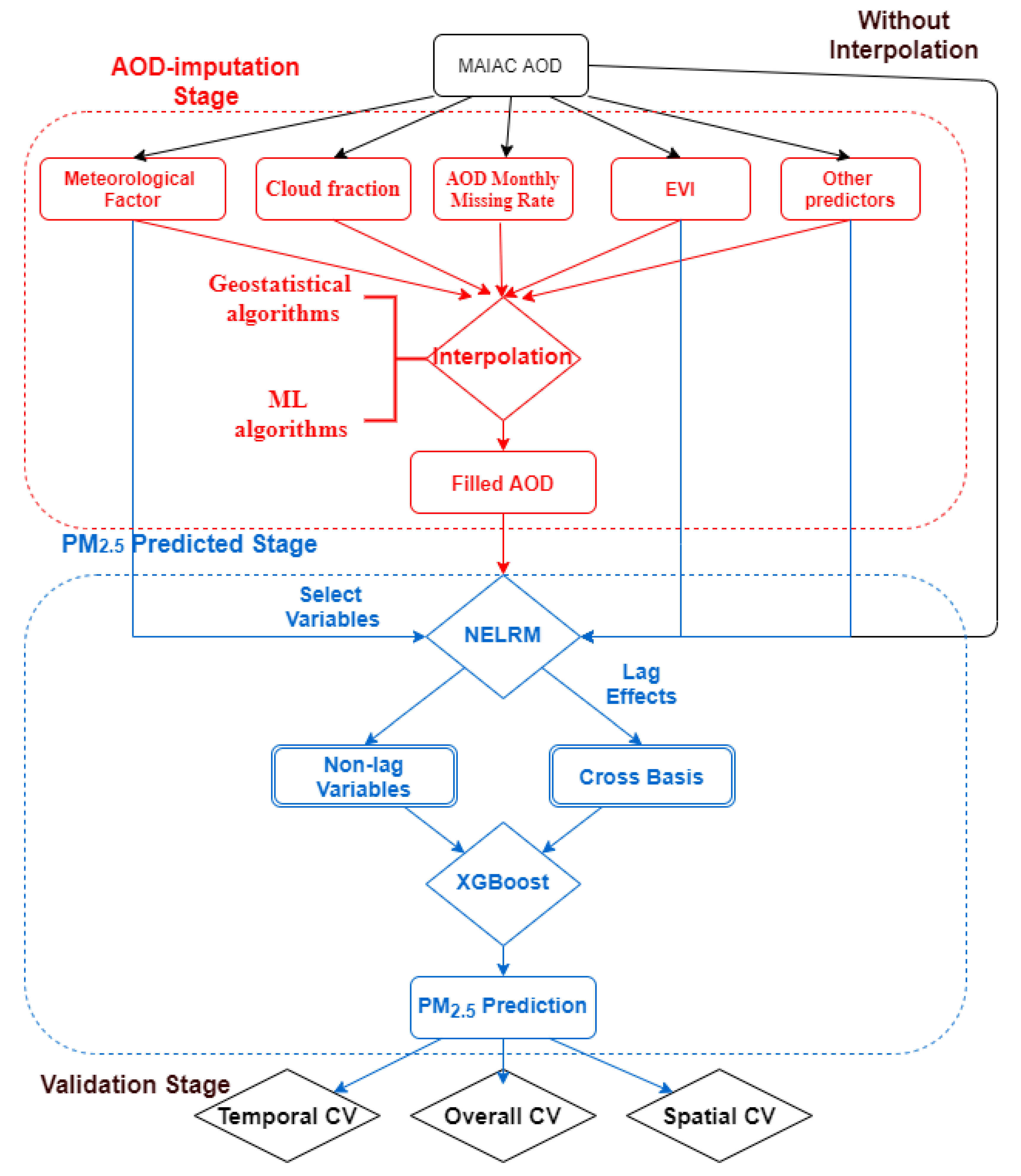
Meteorological data, including the daily mean temperature, pressure, sunshine hours, water vapor pressure, precipitation, relative humidity, wind speed, and wind direction, were obtained from 839 meteorological stations (Figure S1B) during 2013–2018. For further integration, the Universal Kriging (UK) technique was employed to interpolate the daily site-level meteorological data into grid cells with a resolution of 1 km. The 6-hour planetary boundary layer height (PBLH) from the National Centers for Environmental Prediction (NECP) was daily averaged and resampled from 1 degree to 1 km grid cells [9].

2.2. Methodology

The general workflow for estimating daily PM2.5 exposure (including AOD-imputation stage and PM2.5-prediction stage) is demonstrated in Figure 1.

2.2.1. AOD-Imputation Stage for MAIAC AOD

To select the optimal missing-filled methods for MAIAC AOD, we compared all potential methods, if the data required were available. These included different geostatistical interpolations [26,27,28], two-step imputation previously proposed [9] and other ML interpolating methods, including random forest (RF) [29], XGBoost (extreme gradient boosting) [30], support vector machine (SVM) [31], gradient boost model (GBM) [32], generalized additive model (GAM) [33], Bayesian regularized neural network (BRNN) [34], and least absolute shrinkage and selection operator (LASSO) [35]. The interpolation methods are summarized in Table 1. In general, geostatistical algorithms mainly depend on using spatial and temporal information in existing AOD data, while ML algorithms mainly use the complex relationship between AOD and other external information.
Geostatistical algorithms require less information and can suit the situation without requiring external information. In most cases, ML algorithms can provide a model for an entire study period, but geostatistical algorithms need to be conducted separately for each day or at specified intervals because they cannot provide a fixed model for the entire period. The parameter setting used in this study (Table S1) was tuning by 10-fold cross-validation.
For the ML algorithms, the selected predictors among different ML methods remained consistent to compare their performances objectively. All external information was selected by linear models with statistical significance (P < 0.05) and low variance inflation (VIF < 5, checks for multi-collinearity). The external information included PBLH, maximum ground surface temperature (Maxgst), precipitation (rain), maximum atmospheric pressure (Maxpres), mean relative humidity (MeanRH), sunshine duration (sunshine), mean ambient temperature (Meantemp), max/maximum wind speed (WS/MWS), cloud fraction (representing the levels of cloud coverage) from MOD06_L2, AOD monthly missing rate, EVI, and indicator variables such as longitude and latitude, altitude, day of the year, month, year, and day of the week. It should be noted that the sample size of MAIAC AOD covering China from 2013–2018 was too large (approximately 96,534,23 (numbers of grids) × 365 (days) × 6 (years)) to train the missing-filled model, and therefore, 5000 grids were randomly selected for each day as the modeling data (total sample size = 5000 (numbers of grids) × 365 (days) × 6 (years)). The external information for each grid was extracted from the corresponding grid cell.

2.2.2. PM2.5-Prediction Stage

Due to natural geographical differences among the seven geographical regions in China such as climate, terrain, and vegetation [9], a satellite-PM2.5 model was constructed separately for each region. To alleviate the discontinued and less-certainty problem between the regions’ boundaries, the sites in the neighboring province (Figure S2) were also included in the corresponding modeling region.
Our previous PM2.5 prediction model (a combined method of NELRM and XGBoost) [9] worked well at a large spatial scale (CV R2 = 0.86) compared with other ML models (including random forest), and therefore, this study retained a similar PM2.5 model structure. Here, the impacts of different interpolations at the AOD-imputation stage on PM2.5 predictive accuracy are mainly explored, rather than improving PM2.5 model structure. The steps of the NELRM-XGBoost model have been previously described [9] and will be introduced briefly. First, non-lagged variables X 1 such as land-related data, and potential lagged variables X 2 such as original AOD, and meteorological variables were selected in the NELRM [14], with statistical significance (P < 0.05) and low variance inflation (VIF<5, checks for multi-collinearity). The optimal predictor combinations in different regions are shown in Table S2). Additionally, a cross-basis C b . X 2 was constructed, explaining the lag effects, with degree of freedom (df = 3) for natural cubic smooth function and maximum 0–1 lagged days according to the 10-fold CV results. Finally, the weak learner f k X 1 , C b . X 2 in XGBoost learning process was built, which was optimized by the loss function L k θ k , adjusted by a previous iteration, and the regularizing term Ω k θ k , and hence, reducing model complexity for avoiding over fit. This is presented as the following equation:
y ^ i t = k = 1 t ε γ k f k X 1 , C b . X 2
where Y ^ i t denotes PM2.5 estimation in iteration t; γ k and ε are the weight vector and the learning rate. The setting in the satellite-PM2.5 model (Table S1) was optimized by maximizing the 10-fold CV R2 of the XGBoost approach for estimating PM2.5.

2.2.3. Validation Stage

To better validate the performance of two stages, three kinds of 10-fold CV [14], were deployed, including overall CV, spatial CV, and temporal CV. All 10-fold CV were repeated 20 times. The main difference among them was randomly separating the dataset by observations, the location of sites, and date.
The overall CV is a common measurement that represents the performance stability in modeling dataset [13,23,36,37,38].
Spatial CV or spatial extrapolation is a more important indicator of prediction model of PM2.5, because most predicted locations for exposure assessment do not have any observation due to the limited numbers of sites (1605). For a better description of the spatial performance distribution, we also conducted a Leave-One-Out-Cross-Validation (LOOCVsite), which leaves one site for validation each time. The LOOCVsite results were further interpolated by UK into 1 km grids in China (interpolating quality: CV R2 = 0.86), which simply represents spatial extrapolation in different predicted locations.
The temporal CV, or temporal extrapolation means the performance stability in different time points, as the training and validating datasets randomly split by dates in each fold. Furthermore, the validation analysis was performed in different months or years to examine the performance stability (Figure S3).

3. Results

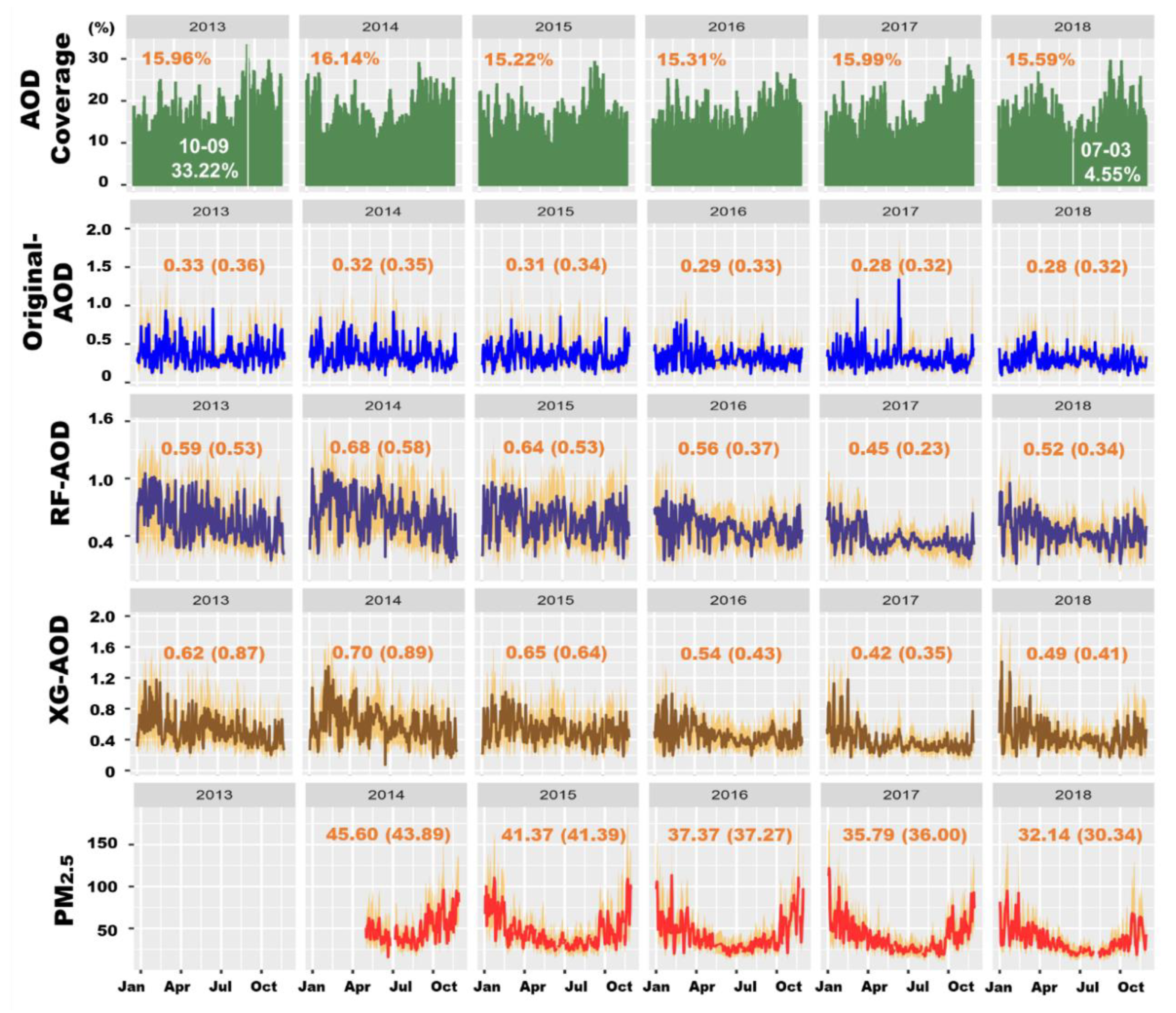
3.1. Descriptive Statistics of MAIAC AOD and PM2.5 Concentration

From 2013 to 2018, the daily coverage of MAIAC AOD in China generally remained at an average of approximately 15–16% (Figure 2). The highest coverage day was on 9 October 2013, reaching 33.22%, and the lowest coverage day was 4.55% on 3 July 2018. June–July and January–February accounted for 42.24% and 28.87% of the lower-coverage (≤10%) days, respectively, and more than 62.31% of the higher-coverage (≥20%) days were from September–December. The median value of the observed MAIAC AOD during the study period was approximately 0.31(interquartile range (IQR): 0.34).
From 2014 to 2018, the median PM2.5 concentrations reported by the monitoring sites gradually decreased from 45.60 μ g / m 3 (IQR = 43.89) to 32.14 μ g / m 3 (IQR = 30.34). The PM2.5 concentrations in China were always higher in the cold season (October–March).

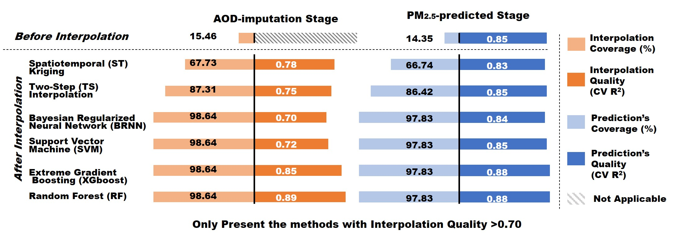
3.2. AOD-Imputation Stage

Compared with the geostatistical interpolation methods (coverage after interpolation approximately 21.43–87.31% for NN, Kriging, IDW, ST Kriging, and TS) (Table 2), the ML methods, using the same external information, were more efficient in filling the gaps, with almost full coverage (approximately 98.64%). The remaining missing data could not be fully eliminated due to the missing rates of external information. Among these algorithms, the RF and XG methods outperformed other algorithms (CV R2 = 0.89, 0.85, and 0.49–0.78 for RF, XG, and other algorithms, respectively). Although the RF method was the most accurate, its computation time was longer than other ML algorithms and most geostatistical algorithms. The XG method was less time-consuming, had better performance, and higher coverage than our previous TS methods, although the accuracy was slightly lower than RF. Similar results were obtained for spatial CV and temporal CV (Table S3). Among the interpolations with higher accuracy (CV R2 ≥ 0.7), we found the median AOD level always tended to increase (from 0.31 to 0.44–0.65) after geostatistical or ML interpolation. Owing to the same coverage in ML-interpolated AOD product (same external information for all ML algorithms), they had a more similar interpolated AOD distribution than the geostatistical interpolation. In addition, the linear correlation between interpolated AOD and PM2.5 weakened after the interpolation (Table S4).

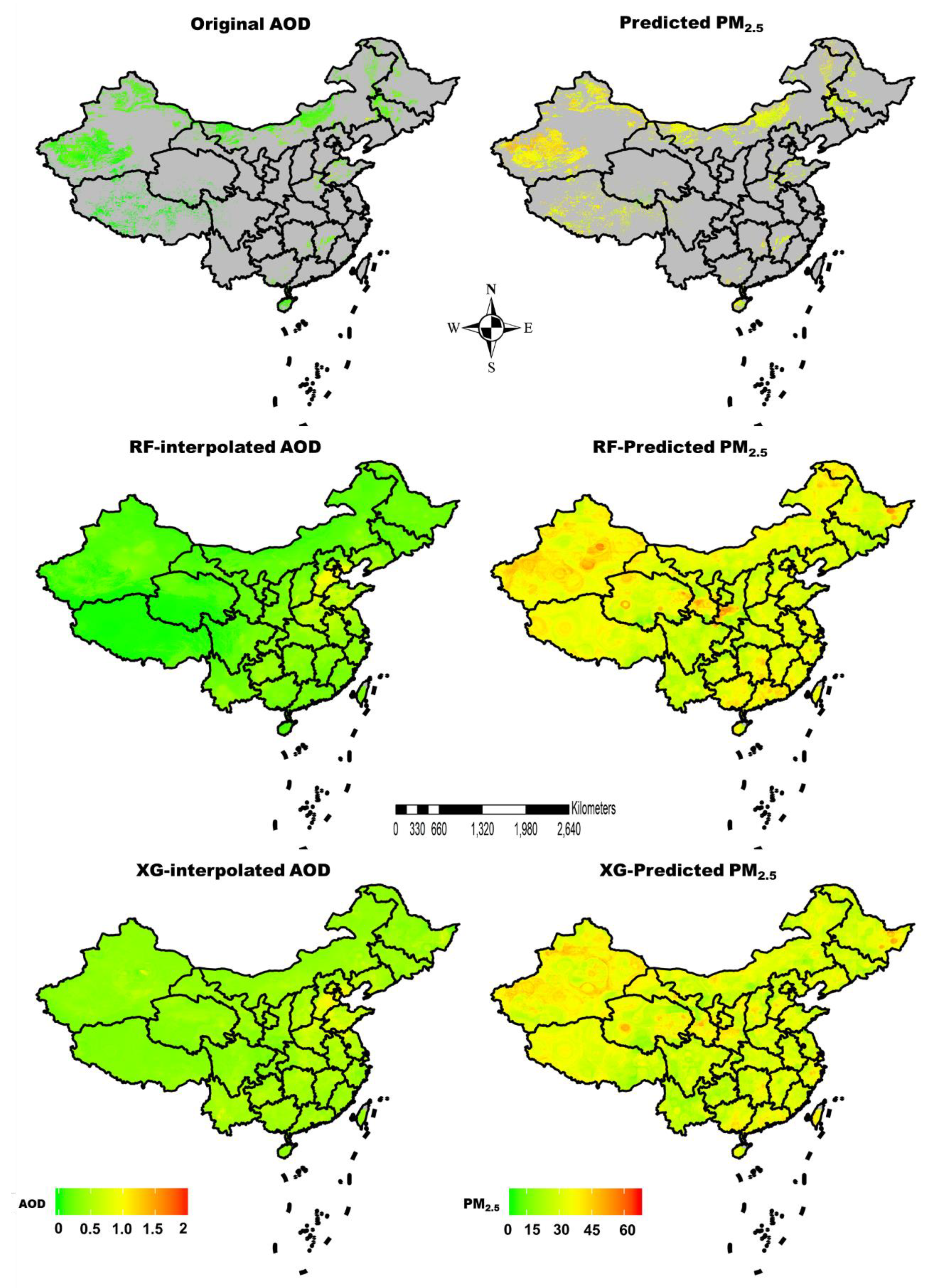
3.3. PM2.5 Predicted Stage

Six AOD-interpolation methods allowed relatively higher performances (with CV R2 after over 0.7), and therefore, their interpolated AOD product was used to build the daily PM2.5 prediction model at the second stage (CV R2: 0.83–0.88) (Table S5). It was found that using AOD products interpolated by XG or RF (XG-AOD or RF-AOD) was beneficial to short-term PM2.5 prediction accuracy (CV R2: both 0.88), and more accurate than when using original AOD data (CV R2: 0.85). We, therefore, further compared XG-AOD and RF-AOD in different regions (Figure 3). Generally, PM2.5 prediction models using either AOD product performed similarly and obtained CV R2 higher than 0.88 in most regions of China, except for the northwest (approximately 0.77–0.78). Using XG-AOD was more stable (lower SD or narrower 95% CI for CV R2) in the northwest. This was similar to spatial CV and temporal CV (spatial (temporal) CV R2 = 0.83(0.83) for RF vs. 0.82(0.82) for XG), while the PM2.5 prediction model using the original AOD had a less stable performance, with a spatial CV R2 of 0.65 and a temporal CV R2 of 0.61 (Table S6).

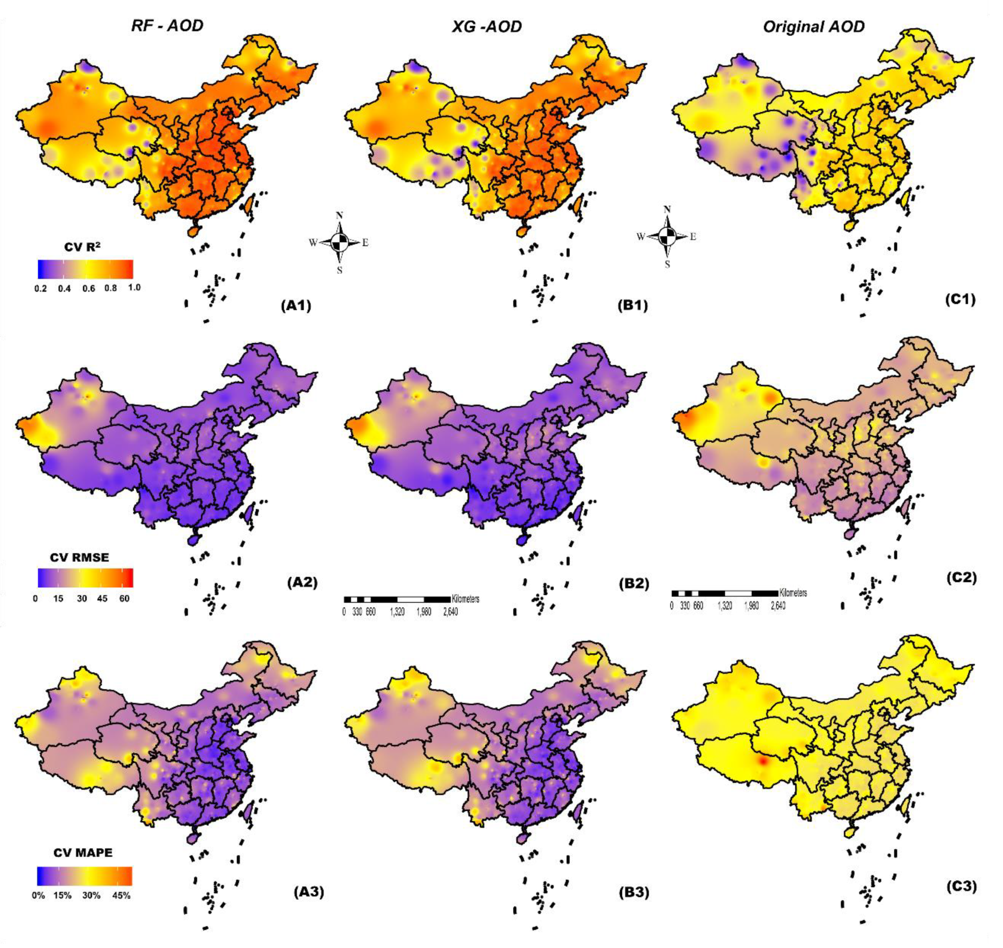
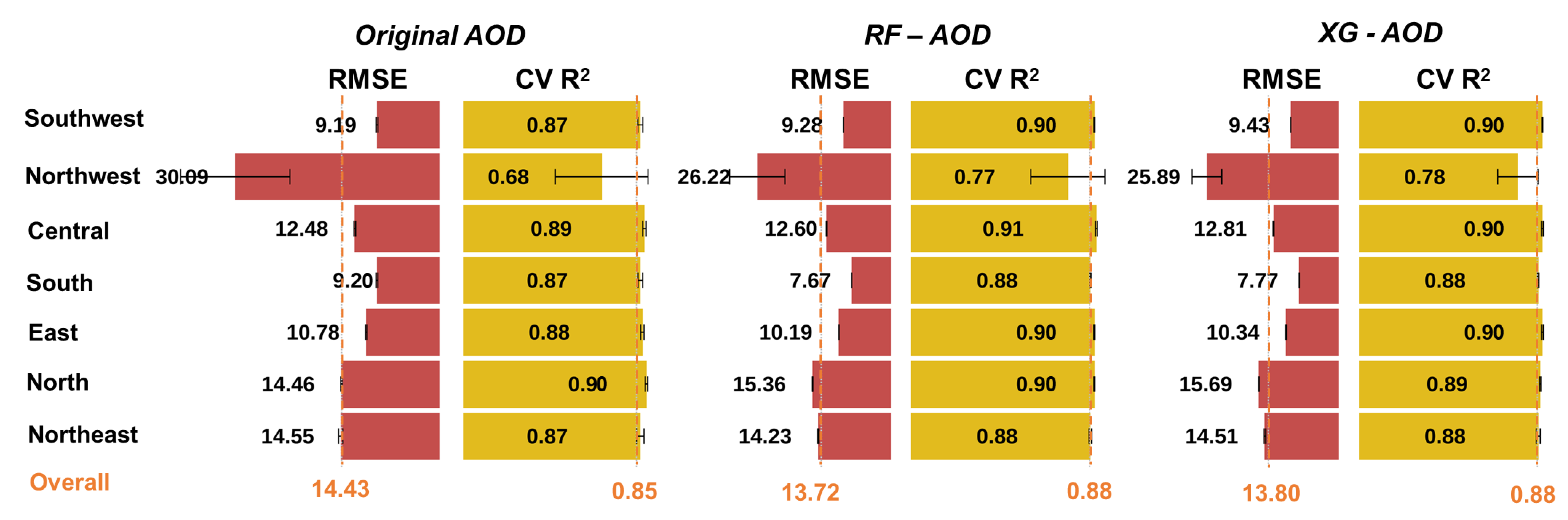
3.4. Spatial and Temporal Cross-Validation

Due to the high demand of spatial extrapolation, a LOOCVsite analysis was conducted (Figure 4). The results were similar while using two different interpolated AOD products at the PM2.5-prediction stage. The model using RF-AOD performed slightly better than XG-AOD (median LOOCV R2 (RMSE): 0.81(14.68 μg/m3) vs. 0.78(15.07 μg/m3), respectively). Both were significantly better than using original AOD (median LOOCV R2 = 0.56, RMSE = 24.48 μg/m3). The grids with higher accuracy (coverage rate and LOOCV R2 > median level) were mainly located in the east of China, including Central, South, East, North, and Northeast China. For temporal CV, the RF or XG interpolation strategy performed significantly better than the original AOD, and they had similar temporal CV among different months or years (Figure S3). The warm season (April–September) generally performed more poorly than the cold season (November–March). The CV result was stable in different years.
To better clarify the performance of the interpolation methods, we specifically illustrated the result under the worst condition during the study period, i.e., when the coverage of MAIAC AOD was the lowest (4.55% on 3 July 2018) (Figure 5). The coverage of AOD could reach 96.25% for both RF- and XG-interpolation (determined by the missing of external information), and median levels of interpolated AOD changed from 0.18 to 0.53 (RF) and to 0.57 (XG). In the meantime, the coverage of predicted PM2.5 increased from 4.12% to 95.46% (determined by the additional missing while considering lag effect), and LOOCVsite R2 of predicted PM2.5 was 0.70 (original), 0.86 (RF), and 0.85 (XG). The median (IQR) levels of PM2.5 ( μ g / m 3 ), estimated by MAIAC AOD, RF-AOD, and XG-AOD, were 36.34 (22.26), 27.52 (25.68), and 26.32 (27.42), respectively.

4. Discussion

This study developed a series of strategies for estimating daily PM2.5 exposure. This included two stages; the AOD-imputation stage and the PM2.5 predicted stage. For the AOD-imputation stage, and to resolve the difficult aspects of our previous two-step interpolation such as relatively tedious steps and ignoring influences of external information [9], this study compared 12 different algorithms and found ML algorithms (with external information) generally achieved higher coverage than geostatistical algorithms (98.64% vs. 21.43–87.31%). The RF or XG interpolation among ML algorithms also guaranteed a higher interpolated quality (CV R2 = 0.89 and 0.85) than other ML algorithms (CV R2 = 0.49–0.72) or geostatistical algorithms (CV R2 = 0.49–0.78). However, XG interpolation can better balance the computation time and performance. Compared with the model using original AOD, the PM2.5 prediction model using XG-AOD not only guaranteed higher coverage (97.83% vs. 14.35%), but also a better prediction performance (CV R2: 0.88 vs. 0.85) for the PM2.5-prediction stage.
The AOD model has provided optimism for high-coverage estimations of PM2.5 exposure to compensate for the very low coverage of existing ground air quality monitoring sites. It was found, however, that the AOD-missing rate was above 84% among the day-grid units in China during 2013–2018, and similar problems have been reported in different regions [14,39,40,41]. This raises debate regarding whether the short-term estimation of PM2.5, based on retrieved AOD data, is more practical for further research rather than data from the sites. For example, in China, PM2.5 predicted by MAIAC AOD still maintains a higher resolution (1 km) and a higher coverage (approximately 96,534,23 grids) than data from the sites (approximately 1605 sites), and the sites are more likely to be concentrated in eastern China, which is densely populated due to economic and social reasons [40]. A similar situation also exists in many developing countries and in high-income countries [42,43]. Missing observations of MAIAC AOD also tend to be concentrated in specific areas due to uncontrollable factors such as orbit patterns and cloudiness [9,10]. For example, in the lowest coverage day (3 July 2018) during the study period, severe convective weather and heavy rainfall in coastal and central areas of China may have led to such an absence. Furthermore, previous studies have suggested that a monsoon climate is associated with more frequently missed observations. The large seasonal variations in the observed aerosol data [17,44] due to more rainy or cloudy weather in the summer [45], means that regions with a monsoon climate, which are concentrated in densely populated areas, are more susceptible to the missing observation problem and therefore, appropriate AOD interpolation is a prerequisite before using the AOD model for higher-coverage assessments of PM2.5 exposure.
Many attempts have previously been made to impute AOD-missing observations, but it remains unclear which is the most optimal. We compared the performances of 12 approaches, including those proposed here, and found ML algorithms using external information can fill more missing data than geostatistical interpolation (approximately 98.64% vs. 21.43–87.31%). This was consistent with previous assumptions [46,47,48], but the interpolation quality (CV R2: 0.49–0.89) varied widely in different algorithms, with a similar range (CV R2 approximately 0.34–0.85) reported in previous different studies [14,15,16,17,43,46,47,48,49,50,51]. The higher missing-filled efficiency of ML algorithms indicates that external information can provide more information at the AOD-imputation stage, because the geostatistical interpolation is over-dependent on spatial autocorrelation but ignores other influencing factors on the temporal dimension [21]. Not all ML algorithms, however, can obtain higher interpolation quality than geostatistical interpolation, and the varied interpolation quality suggests that the model structure, or the ability to capture complex spatio-temporal relationships rather than external information, plays a more important role in the accuracy of the AOD-filled process. Therefore, suitable ML algorithms were selected by 10-fold cross-validation. Most geostatistical interpolations could not provide a fixed model for the entire period, that is, they needed to be developed separately for each map slice at different time points, and so tended to take a longer running time. Among different interpolations, the RF and XG methods were the best two groups, with the highest CV R2 (0.89 and 0.85, respectively), but the time consumption of the RF method was much longer due to parallel operation and different calculation methods. Furthermore, the RF method consumed more memory during computation. It is necessary to tradeoff time consumption and interpolation quality if robust computing power is not available.
It was also found that the average AOD levels always rose after interpolation, irrespective of the interpolating method used. This is consistent with the phenomenon that missing more frequently occurs at high MODIS-AOD levels [52,53]. The aerosol hygroscopic growth during missing days results from increased humidity from cloud or humid airflows [54,55]. Another potential reason is that the surface reflectivity, cloudiness, or snow is always associated with over-exposure values [9,10], so it tends to be eliminated during the preprocess of satellite sensors or systems. It was also found that PM2.5 levels on AOD-missing days were lower than those on non-missing days (36.0   μ g / m 3 vs. 39.0   μ g / m 3 ), and this was partially due to shorter particle suspension time with heavy rainfall, convective weather or snow [56], and higher missing rates in the warm season (April–September), with relatively lower PM2.5 levels (Figure 2). This suggests that the relationship between AOD and PM2.5 after AOD interpolation, becomes more complicated than a simple linear relationship [9]. This could explain why AOD interpolation can lead to weaker linear correlations (0.43 to 0.31) (Table S4) but higher accuracy in our PM2.5 prediction model, which can capture the complicated spatio-temporal variations (0.85 to 0.88) (Figure 3).
At the PM2.5 predicted stage, further discussion is required regarding how many benefits can be obtained from different interpolated AOD products. Compared with non-AOD model, the imputed AOD always improves the accuracy of PM2.5 estimation (CV R2 PM2.5 estimation = 0.77 vs. 0.83~0.88) (Table S5), especially for XG and RF interpolations which had higher interpolating quality (CV R2 AOD imputation > 0.8). Furthermore, compared with RF-AOD and XG-AOD, the satellite PM2.5 model using original AOD performed relatively poorly in spatial and temporal CVs (spatial (temporal) CV R2 = 0.83(0.83) vs. 0.82(0.82) vs. 0.65(0.61)). The lower LOOCV R2 (=0.56) when only using original AOD further proved its poorer spatial application to all mainland China because different missing rates in different grids can increase the heterogeneity (or uncertainty) of predictions, and further weaken spatial extrapolation to other grids. Furthermore, incomplete time series of AOD produced for each grid also makes it more difficult to obtain an accurate prediction in any out-of-sample time. Compared with the XG method, however, the higher accuracy of RF methods at the AOD-imputation stage did not bring more benefits to the PM2.5-prediction stage. It indicated that the missing rate of the AOD product, compared with the accuracy of the interpolated AOD product, is the key to spatial and temporal extrapolation of the PM2.5-prediction stage.
Some limitations were present in this study. First, the complex relationships between AOD-missing effect and PM2.5 may cause annual and regional differences, which need to be further analyzed in more countries for a longer research period. Second, the AOD miss-filling approaches taken here are based on using known predictors which are easily accessed and are frequently recorded in most areas and therefore, some other chemical or physical features such as chemical composition in aerosol and sun radiation were not considered in this study. Finally, the LOOCV result for all of China was interpolated by UK, and therefore, some unavoidable bias due to the UK technique may be present. This result provides an approximate assessment only for spatial dimensions.

5. Conclusions

This study proposed a XGBoost method to impute missing data of AOD based on some external predictors. By comparing a variety of different imputation methods, XGBoost is confirmed to be a less consuming-time choice, with almost full coverage, good missing-imputation quality, and consequently, accurate prediction of PM2.5. In terms of practicality, our study provides some guidance, strategies, and a tempo-spatially continuous PM2.5 dataset for future short-term health impact assessments in epidemiological studies of air pollution.

Supplementary Materials

The following are available online at https://www.mdpi.com/2072-4292/12/18/3008/s1, Figure S1. Geographical distribution of PM2.5 monitoring sites (A) and meteorological stations (B) in mainland China in 2015. Figure S2. Geographical locations of regions and provinces in China. Figure S3. The temporal CV performance (Proportion of sites with different CV R2) of daily Satellite-PM2.5 model in China with RF-AOD, XG-AOD and Original AOD. Table S1. The optimal parameters selected in AOD-filled Stage and PM2.5 Predicted Stage. Table S2. Optimal combination of variables selected in different regions of China. Table S3. The spatial and temporal CV of Geostatistical and ML interpolation for MAIAC AOD product. The comparison of daily Satellite-PM2.5 model with AOD products interpolated by using interpolating methods (with CV R2 for interpolation > = 0.7). Table S6. The spatial and temporal CV of using different interpolated-AOD product in PM2.5 Predicted Stage.

Author Contributions

Conceptualization, Z.-Y.C., J.-Q.J., R.Z., T.-H.Z., J.-J.C., J.Y., C.-Q.O. and Y.G.; Data curation, Z.-Y.C., J.-Q.J., J.-J.C. and J.Y.; Formal analysis, Z.-Y.C.; Funding acquisition, C.-Q.O. and Y.G.; Methodology, Z.-Y.C., R.Z. and C.-Q.O.; Project administration, Z.-Y.C., C.-Q.O. and Y.G.; Software, Z.-Y.C.; Supervision, C.-Q.O. and Y.G.; Validation, Z.-Y.C., J.-Q.J., R.Z. and T.-H.Z.; Writing—original draft, Z.-Y.C.; Writing—review and editing, Z.-Y.C., C.-Q.O. and Y.G. All authors have read and agreed to the published version of the manuscript.

Funding

This research was funded by National Nature Science Foundation of China [81573249], Nature Science Foundation of Guangdong Province [2016A030313530] and Australian National Health and Medical Research Council [APP1107107]. And The APC was funded by National Nature Science Foundation of China [81573249] and Nature Science Foundation of Guangdong Province [2016A030313530].

Acknowledgments

This study was supported by National Nature Science Foundation of China [81573249], Nature Science Foundation of Guangdong Province [2016A030313530]. YG was supported by Career Development Fellowship of Australian National Health and Medical Research Council [APP1107107].

Conflicts of Interest

The authors declare no conflict of interest.

References

  1. International Energy Agency. Key World Energy Statistics 2018; OECD Publishing: Paris, France, 2018. [Google Scholar]
  2. Cohen, A.J.; Brauer, M.; Burnett, R.; Anderson, H.R.; Frostad, J.; Estep, K.; Balakrishnan, K.; Brunekreef, B.; Dandona, L.; Dandona, R.; et al. Estimates and 25-year trends of the global burden of disease attributable to ambient air pollution: An analysis of data from the Global Burden of Diseases Study 2015. Lancet 2017, 389, 1907–1918. [Google Scholar] [CrossRef] [Green Version]
  3. Lee, S.; Lee, W.; Kim, D.; Kim, E.; Myung, W.; Kim, S.-Y.; Kim, H. Short-term PM2.5 exposure and emergency hospital admissions for mental disease. Environ. Res. 2019, 171, 313–320. [Google Scholar] [CrossRef]
  4. Shah, A.S.V.; Lee, K.K.; McAllister, D.A.; Hunter, A.; Nair, H.; Whiteley, W.; Langrish, J.P.; Newby, D.E.; Mills, N.L. Short term exposure to air pollution and stroke: Systematic review and meta-analysis. BMJ 2015, 350, h1295. [Google Scholar] [CrossRef] [PubMed] [Green Version]
  5. Guaita, R.; Pichiule, M.; Maté, T.; Linares, C.; Díaz, J. Short-term impact of particulate matter (PM2.5) on respiratory mortality in Madrid. Int. J. Environ. Health Res. 2011, 21, 260–274. [Google Scholar] [CrossRef] [PubMed]
  6. Kloog, I.; Ridgway, B.; Koutrakis, P.; Coull, B.A.; Schwartz, J.D. Long-and short-term exposure to PM2.5 and mortality: Using novel exposure models. Epidemiology 2013, 24, 555. [Google Scholar] [CrossRef] [PubMed]
  7. Mar, T.F.; Jansen, K.; Shepherd, K.; Lumley, T.; Larson, T.V.; Koenig, J.Q. Exhaled nitric oxide in children with asthma and short-term PM2.5 exposure in Seattle. Environ. Health Perspect. 2005, 113, 1791–1794. [Google Scholar] [CrossRef] [Green Version]
  8. WHO. Air Quality Deteriorating in Many of the World’s Cities; WHO: Geneva, Switzerland, 2014. [Google Scholar]
  9. Chen, Z.-Y.; Zhang, T.-H.; Zhang, R.; Zhu, Z.-M.; Yang, J.; Chen, P.-Y.; Ou, C.-Q.; Guo, Y. Extreme gradient boosting model to estimate PM2.5 concentrations with missing-filled satellite data in China. Atmos. Environ. 2019, 202, 180–189. [Google Scholar] [CrossRef]
  10. Kahn, R.A.; Nelson, D.L.; Garay, M.J.; Levy, R.C.; Bull, M.A.; Diner, D.J.; Martonchik, J.V.; Paradise, S.R.; Hansen, E.G.; Remer, L.A. MISR aerosol product attributes and statistical comparisons with MODIS. IEEE Trans. Geosci. Remote Sens. 2009, 47, 4095–4114. [Google Scholar] [CrossRef]
  11. Paciorek, C.J.; Liu, Y. Limitations of remotely sensed aerosol as a spatial proxy for fine particulate matter. Environ. Health Perspect. 2009, 117, 904–909. [Google Scholar] [CrossRef] [Green Version]
  12. Zhang, T.; Gong, W.; Zhu, Z.; Sun, K.; Huang, Y.; Ji, Y. Semi-physical estimates of national-scale PM10 concentrations in China using a satellite-based geographically weighted regression model. Atmosphere 2016, 7, 88. [Google Scholar] [CrossRef] [Green Version]
  13. Liu, Y.; Paciorek, C.J.; Koutrakis, P. Estimating regional spatial and temporal variability of PM2.5 concentrations using satellite data, meteorology, and land use information. Environ. Health Perspect. 2009, 117, 886. [Google Scholar] [CrossRef] [PubMed] [Green Version]
  14. Chen, Z.; Zhang, T.; Zhang, R.; Zhu, Z.; Ou, C.; Guo, Y. Estimating PM2.5 concentrations based on non-linear exposure-lag-response associations with aerosol optical depth and meteorological measures. Atmos. Environ. 2018, 173, 30–37. [Google Scholar] [CrossRef]
  15. Kloog, I.; Koutrakis, P.; Coull, B.A.; Lee, H.J.; Schwartz, J. Assessing temporally and spatially resolved PM 2.5 exposures for epidemiological studies using satellite aerosol optical depth measurements. Atmos. Environ. 2011, 45, 6267–6275. [Google Scholar] [CrossRef]
  16. Lv, B.; Hu, Y.; Chang, H.H.; Russell, A.G.; Bai, Y. Improving the accuracy of daily PM2.5 distributions derived from the fusion of ground-level measurements with aerosol optical depth observations, a case study in North China. Environ. Sci. Technol. 2016, 50, 4752. [Google Scholar] [CrossRef]
  17. Xiao, Q.Y.; Wang, Y.; Howard, H.C.; Xia, M.; Geng, G. Full-coverage high-resolution daily PM2.5 estimation using MAIAC AOD in the Yangtze River Delta of China. Remote Sens. Environ. 2017, 199, 437–446. [Google Scholar] [CrossRef]
  18. Di, Q.; Kloog, I.; Koutrakis, P.; Lyapustin, A.; Wang, Y.; Schwartz, J. Assessing PM2.5 exposures with high spatiotemporal resolution across the continental United States. Environ. Sci. Technol. 2016, 50, 4712–4721. [Google Scholar] [CrossRef] [Green Version]
  19. Lyapustin, A.; Wang, Y.; Laszlo, I.; Kahn, R.; Korkin, S.; Remer, L.; Levy, R.; Reid, J. Multiangle implementation of atmospheric correction (MAIAC): 2. Aerosol algorithm. J. Geophys. Res. 2011, 116. [Google Scholar] [CrossRef]
  20. Lyapustin, A.; Wang, Y.; Korkin, S.; Huang, D. MODIS Collection 6 MAIAC algorithm. Atmos. Meas. Tech. 2018, 11, 5741–5765. [Google Scholar] [CrossRef] [Green Version]
  21. Li, L.; Franklin, M.; Girguis, M.; Lurmann, F.; Wu, J.; Pavlovic, N.; Breton, C.; Gilliland, F.; Habre, R. Spatiotemporal imputation of MAIAC AOD using deep learning with downscaling. Remote Sens. Environ. 2020, 237, 111584. [Google Scholar] [CrossRef]
  22. Zhang, Z.; Wu, W.; Fan, M.; Wei, J.; Tan, Y.; Wang, Q. Evaluation of MAIAC aerosol retrievals over China. Atmos. Environ. 2019, 202, 8–16. [Google Scholar] [CrossRef]
  23. Hu, X.; Waller, L.A.; Lyapustin, A.; Wang, Y.; Al-Hamdan, M.Z.; Crosson, W.L.; Estes, M.G., Jr.; Estes, S.M.; Quattrochi, D.A.; Puttaswamy, S.J. Estimating ground-level PM2.5 concentrations in the Southeastern United States using MAIAC AOD retrievals and a two-stage model. Remote Sens. Environ. 2014, 140, 220–232. [Google Scholar] [CrossRef]
  24. CHINA MEE. Ambient Air Quality Standardss.GB 3095-2012; China Environmental: Beijing, China, 2016. [Google Scholar]
  25. San Martini, F.M.; Hasenkopf, C.A.; Roberts, D.C. Statistical analysis of PM2.5 observations from diplomatic facilities in China. Atmos. Environ. 2015, 110, 174–185. [Google Scholar] [CrossRef]
  26. Lv, B.; Hu, Y.; Chang, H.H.; Russell, A.G.; Cai, J.; Xu, B.; Bai, Y. Daily estimation of ground-level PM2.5 concentrations at 4 km resolution over Beijing-Tianjin-Hebei by fusing MODIS AOD and ground observations. Sci. Total Environ. 2017, 580, 235–244. [Google Scholar] [CrossRef] [PubMed]
  27. Zhu, X.; Liu, D.; Chen, J. A new geostatistical approach for filling gaps in Landsat ETM+ SLC-off images. Remote Sens. Environ. 2012, 124, 49–60. [Google Scholar] [CrossRef]
  28. Wikle, C.; Zammit-Mangion, A.; Cressie, N. Spatio-Temporal Statistics with R; CRC Press: Boca Raton, FL, USA, 2019; ISBN 9781351769723. [Google Scholar]
  29. Liaw, A.; Wiener, M. Classification and regression by RandomForest. R News 2002, 2, 18–22. [Google Scholar]
  30. Chen, T.; Guestrin, C. XGBoost: A scalable tree boosting system. Knowl. Discov. Data Min. 2016, 785–794. [Google Scholar] [CrossRef] [Green Version]
  31. Wang, L. Support Vector Machines: Theory and Applications; Springer Science & Business Media: Berlin/Heidelberg, Germany, 2005; Volume 177, p. 3887. [Google Scholar]
  32. Ridgeway, G. Generalized Boosted Models: A guide to the gbm package. Update 2007, 1, 2007. [Google Scholar]
  33. Brenning, A. Statistical geocomputing combining R and SAGA: The example of landslide susceptibility analysis with generalized additive models. Hamburg. Beiträge zur Phys. Geogr. und Landschaftsökologie 2008, 19, 410. [Google Scholar]
  34. Pérez-Rodríguez, P.; Gianola, D.; Weigel, K.A.; Rosa, G.J.M.; Crossa, J. An R package for fitting Bayesian regularized neural networks with applications in animal breeding. J. Anim. Sci. 2013, 91, 3522–3531. [Google Scholar] [CrossRef] [Green Version]
  35. Kuhn, M. Building predictive models in R using the caret package. J. Stat. Softw. 2008, 28, 1–26. [Google Scholar] [CrossRef] [Green Version]
  36. Just, A.C.; De Carli, M.M.; Shtein, A.; Dorman, M.; Lyapustin, A.; Kloog, I. Correcting measurement error in satellite aerosol optical depth with machine learning for modeling PM2.5 in the Northeastern USA. Remote Sens. 2018, 10, 803. [Google Scholar] [CrossRef] [PubMed] [Green Version]
  37. He, Q.; Huang, B. Satellite-based mapping of daily high-resolution ground PM2.5 in China via space-time regression modeling. Remote Sens. Environ. 2018, 206, 72–83. [Google Scholar] [CrossRef]
  38. Xue, T.; Zheng, Y.; Geng, G.; Zheng, B.; Jiang, X.; Zhang, Q.; He, K. Fusing observational, satellite remote sensing and air quality model simulated data to estimate spatiotemporal variations of PM2.5 exposure in China. Remote Sens. 2017, 9, 221. [Google Scholar] [CrossRef] [Green Version]
  39. Belle, J.; Liu, Y. Evaluation of Aqua MODIS Collection 6 AOD parameters for air quality research over the Continental United States. Remote Sens. 2016, 8, 815. [Google Scholar] [CrossRef] [Green Version]
  40. You, W.; Zang, Z.; Zhang, L.; Li, Y.; Pan, X.; Wang, W. National-scale estimates of ground-level PM2.5 concentration in China using geographically weighted regression based on 3 km resolution MODIS AOD. Remote Sens. 2016, 8, 184. [Google Scholar] [CrossRef] [Green Version]
  41. Zhang, T.; Gong, W.; Wang, W.; Ji, Y.; Zhu, Z.; Huang, Y. Ground Level PM2.5 Estimates over China Using Satellite-Based Geographically Weighted Regression (GWR) Models Are Improved by Including NO2 and Enhanced Vegetation Index (EVI). Int. J. Environ. Res. Public Health 2016, 13, 1215. [Google Scholar] [CrossRef]
  42. Kim, M.; Zhang, X.; Holt, J.B.; Liu, Y. Spatio-Temporal Variations in the Associations between Hourly PM2.5 and Aerosol Optical Depth (AOD) from MODIS Sensors on Terra and Aqua. Health 2013, 5, 8–13. [Google Scholar] [CrossRef]
  43. McGuinn, L.; Schneider, A.E.; Ward-Caviness, C.; Di, Q.; Schwartz, J.D.; Russell, A.; Hauser, E.; Kraus, W.; Neas, L.; Cascio, W. Comparison of Long-Term PM2.5 Concentrations from Ground-Based Monitoring, CMAQ Models and Satellite-Derived AOD to Characterize Adverse Cardiovascular Outcomes. In ISEE Conference Abstracts; Environmental Health Perspectives: Ottawa, Canada, 2018; Volume 2018. [Google Scholar]
  44. Liu, X.; Yan, L.; Yang, P.; Yin, Z.-Y.; North, G.R. Influence of Indian summer monsoon on aerosol loading in East Asia. J. Appl. Meteorol. Climatol. 2011, 50, 523–533. [Google Scholar] [CrossRef] [Green Version]
  45. Li, Z.; Lau, W.; Ramanathan, V.; Wu, G.; Ding, Y.; Manoj, M.G.; Liu, J.; Qian, Y.; Li, J.; Zhou, T. Aerosol and monsoon climate interactions over Asia. Rev. Geophys. 2016, 54, 866–929. [Google Scholar] [CrossRef]
  46. Zhang, R.; Di, B.; Luo, Y.; Deng, X.; Grieneisen, M.L.; Wang, Z.; Yao, G.; Zhan, Y. A nonparametric approach to filling gaps in satellite-retrieved aerosol optical depth for estimating ambient PM2.5 levels. Environ. Pollut. 2018, 243, 998–1007. [Google Scholar] [CrossRef]
  47. Yang, J.; Hu, M. Filling the missing data gaps of daily MODIS AOD using spatiotemporal interpolation. Sci. Total Environ. 2018, 633, 677. [Google Scholar] [CrossRef] [PubMed]
  48. Goldberg, D.L.; Gupta, P.; Wang, K.; Jena, C.; Zhang, Y.; Lu, Z.; Streets, D.G. Using gap-filled MAIAC AOD and WRF-Chem to estimate daily PM2.5 concentrations at 1 km resolution in the Eastern United States. Atmos. Environ. 2019, 199, 443–452. [Google Scholar] [CrossRef]
  49. Sorek-Hamer, M.; Strawa, A.W.; Chatfield, R.B.; Esswein, R.; Cohen, A.; Broday, D.M. Improved retrieval of PM2.5 from satellite data products using non-linear methods. Environ. Pollut. 2013, 182, 417–423. [Google Scholar] [CrossRef] [PubMed]
  50. Geng, G.; Zhang, Q.; Martin, R.V.; van Donkelaar, A.; Huo, H.; Che, H.; Lin, J.; He, K. Estimating long-term PM2.5 concentrations in China using satellite-based aerosol optical depth and a chemical transport model. Remote Sens. Environ. 2015, 166, 262–270. [Google Scholar] [CrossRef]
  51. Liu, Y.; He, K.; Li, S.; Wang, Z.; Christiani, D.C.; Koutrakis, P. A statistical model to evaluate the effectiveness of PM2.5 emissions control during the Beijing 2008 Olympic Games. Environ. Int. 2012, 44, 100–105. [Google Scholar] [CrossRef]
  52. He, Q.; Li, C.; Tang, X.; Li, H.; Geng, F.; Wu, Y. Validation of MODIS derived aerosol optical depth over the Yangtze River Delta in China. Remote Sens. Environ. 2010, 114, 1649–1661. [Google Scholar] [CrossRef]
  53. Zhang, T.; Zhu, Z.; Gong, W.; Zhu, Z.; Sun, K.; Wang, L.; Huang, Y.; Mao, F.; Shen, H.; Li, Z. Estimation of ultrahigh resolution PM2.5 concentrations in urban areas using 160 m Gaofen-1 AOD retrievals. Remote Sens. Environ. 2018, 216, 91–104. [Google Scholar] [CrossRef]
  54. Na, K.; Kumar, K.R.; Yan, Y.; Diao, Y.; Yu, X. Correlation Analysis between AOD and Cloud Parameters to Study Their Relationship over China Using MODIS Data (2003–2013): Impact on Cloud Formation and Climate Change. Aerosol Air Qual. Res. 2014, 15, 958–973. [Google Scholar]
  55. Bi, J.; Belle, J.H.; Wang, Y.; Lyapustin, A.I.; Wildani, A.; Liu, Y. Impacts of snow and cloud covers on satellite-derived PM2.5 levels. Remote Sens. Environ. 2019, 221, 665–674. [Google Scholar] [CrossRef]
  56. Feng, X.; Wang, S. Influence of different weather events on concentrations of particulate matter with different sizes in Lanzhou, China. J. Environ. Sci. 2012, 24, 665–674. [Google Scholar] [CrossRef]
Figure 1. Framework for short-term PM2.5 exposure estimation.
Remotesensing 12 03008 g001
Figure 2. Descriptive statistics (coverage (%) and median (IQR)) of MAIAC AOD product, interpolated AOD, and observed ground-level PM2.5 concentrations.
Remotesensing 12 03008 g002
Figure 3. Cross-validation performance of PM2.5 prediction model with AOD products interpolated by using random forest (RF) and extreme gradient boosting (XG). Orange dashed line: the overall performance; error bar: 95% CI.
Remotesensing 12 03008 g003
Figure 4. Leave-One-Out-Cross-Validation (LOOCV) performance (CV R2, RMSE and MAPE) of daily PM2.5-prediction models in China using RF-AOD (A1A3), XG-AOD (B1B3), and original AOD (C1C3).
Remotesensing 12 03008 g004
Figure 5. Levels of the observed and interpolated MAIAC AOD, and predicted PM2.5 on 3 July 2018, with the lowest coverage of observed AOD.
Remotesensing 12 03008 g005
Table 1. Summary table of different interpolation methods at the AOD-imputation stage.
MethodsMain FeaturesMeritsDemerits
Geostatistical Algorithms
TS [9]step I: mixed effect model
Step II: IDW
using different satellite productsmore steps
ST Kriging [28]regionalize spatio-temporal variable to obtain semi-variance for krigingmaximize use
spatio-temporal neighborhood information
extensive computation for large spatial and temporal scale
IDW [28]inversed distance weighted-average within search radiuseasier and quicker to calculatedless accurate for
complex spatial distribution
Kriging [28]using semi-variance to explore spatial distribution within search radiuscommonly usednot considering temporal variation
NN [28]nearest neighbors within search radiuseasiest and quickest to calculateless spatial variation
Machine Learning Algorithms
LASSO [35]L1 regularization term was used to penalize nonessential or correlated features in modelprevent over fitting and ensure generalizationdifficult to capture complex non-linear or interacting relationship
GAM [33]use smooth functions to describe the relationshipfit non-linear relationshipeasier to over fit
GBM [32]an ensemble of weak prediction models, such as decision trees.optimized by negative gradient of loss function.over fitting and more computation time
BRNN [34]Bayesian Inference was used to regularize the Maximum Likelihood in Neural Nets
(similar regularization in Ridge Regression)
more robust than standard back-propagation netshigher computation than L1 regularization
SVM [31]Using kernel to map data into higher dimension, and then to fit the error within a certain thresholdproduces higher accuracy with less computation powerweaker extrapolating ability in data with more noise
RF [29]a meta estimator with numbers of classifying decision trees based on different sub-samplescontrol the overfitting by sub-samplesmore computation time
XG [30]a weighted ensemble of weak prediction models with regularized boosting and parallel processingregularized boosting and parallel processingless stable results in early stopping
TS (two-step interpolation), ST Kriging (spatio-temporal kriging with 50 km buffer), IDW (inverse distance weighting with 50 km buffer), NN (nearest neighbors with 30 km buffer), LASSO (Least absolute shrinkage and selection operator), GAM (generalized additive model), GBM (gradient boost model), BRNN (Bayesian regularized neural network), SVM (support vector machine), RF (conditional inference random forest), and XG (extreme gradient boosting).
Table 2. Comparison of geostatistical and machine learning (ML) interpolation for MAIAC AOD product.
Interpolation MethodCoverage (%)Computation Time aCV RMSECV R2CV MAPE (%)
Before Interpolation15.46\
Geostatistical Algorithms
TS87.3155:38:56.560.170.7520.56
ST Kriging67.73128:56:43.560.170.7820.36
IDW45.2245:35:28.390.180.6521.35
Kriging42.3788:46:37.240.170.6620.89
NN21.4315:39:27.930.190.4925.38
ML Algorithms
RF98.64120:55:28.650.150.8918.00
XG98.6418:00:38.200.150.8519.06
SVM98.6419:04:47.640.170.7219.41
BRNN98.6418:45:36.220.170.7022.39
GBM98.6406:35:47.650.180.6925.17
GAM98.6401:05:38.200.170.6221.88
LASSO98.6401:18:30.230.190.4928.03
TS (two-step interpolation), IDW (inverse distance weighting), ST Kriging (spatio-temporal kriging), NN (nearest neighbors with 30 km buffer), RF (Conditional Inference Random Forest), XG (extreme gradient boosting, XGBoost), SVM (support vector machine), BRNN (Bayesian regularized neural network), GBM (gradient boost model), GAM (generalized additive model), and LASSO (least absolute shrinkage and selection operator); a tested by Windows 10 system in 3.4 GHz computer with 16 GB of RAM.

