Article

Incorporating Deep Features into GEOBIA Paradigm for Remote Sensing Imagery Classification: A Patch-Based Approach

Institute of Remote Sensing and GIS, Peking University, Beijing 100871, China
*
Author to whom correspondence should be addressed.
Remote Sens. 2020, 12(18), 3007; https://doi.org/10.3390/rs12183007
Submission received: 13 August 2020 / Revised: 9 September 2020 / Accepted: 11 September 2020 / Published: 15 September 2020

Abstract

:
The fast and accurate creation of land use/land cover maps from very-high-resolution (VHR) remote sensing imagery is crucial for urban planning and environmental monitoring. Geographic object-based image analysis methods (GEOBIA) provide an effective solution using image objects instead of individual pixels in VHR remote sensing imagery analysis. Simultaneously, convolutional neural networks (CNN) have been widely used in the image processing field because of their powerful feature extraction capabilities. This study presents a patch-based strategy for integrating deep features into GEOBIA for VHR remote sensing imagery classification. To extract deep features from irregular image objects through CNN, a patch-based approach is proposed for representing image objects and learning patch-based deep features, and a deep features aggregation method is proposed for aggregating patch-based deep features into object-based deep features. Finally, both object and deep features are integrated into a GEOBIA paradigm for classifying image objects. We explored the influences of segmentation scales and patch sizes in our method and explored the effectiveness of deep and object features in classification. Moreover, we performed 5-fold stratified cross validations 50 times to explore the uncertainty of our method. Additionally, we explored the importance of deep feature aggregation, and we evaluated our method by comparing it with three state-of-the-art methods in a Beijing dataset and Zurich dataset. The results indicate that smaller segmentation scales were more conducive to VHR remote sensing imagery classification, and it was not appropriate to select too large or too small patches as the patch size should be determined by imagery and its resolution. Moreover, we found that deep features are more effective than object features, while object features still matter for image classification, and deep feature aggregation is a critical step in our method. Finally, our method can achieve the highest overall accuracies compared with the state-of-the-art methods, and the overall accuracies are 91.21% for the Beijing dataset and 99.05% for the Zurich dataset.

Graphical Abstract

1. Introduction

Due to its real-time and low-cost, land use/land cover (LULC) mapping using remote sensing images has received widespread attention in recent decades [1]. With the developments in remote sensing technologies, the spatial resolution of remote sensing images becomes increasingly finer, which not only provides new opportunities for mapping LULC with more detailed resolution [2] but also brings some new challenges. Ground entities in very-high-resolution (VHR) imagery often appear to have complex structures, demonstrating the increased heterogeneities within ground entities, interclass similarities and intraclass differences, thus hindering LULC mapping [3,4]. Therefore, there is a high demand for an effective VHR image classification strategy to resolve these challenges.
With the resolution of remote sensing images becoming increasingly finer, image analysis methods shift from pixel-based images analysis (PBIA) to geographic object-based image analysis (GEOBIA) [5]. PBIA methods directly extract features from pixels and then classify each pixel. Differently, GEOBIA methods first segment remote sensing images into homogeneous image objects, then extract features for image objects, and finally classify image objects. Compared with PBIA, GEOBIA has three advantages: (1) The basic unit of image analysis is not a pixel but an image object, which is more in line with human cognition. (2) Image objects can greatly reduce the internal heterogeneity of ground entities because ground entities are much larger than pixels in size, thus further reducing the “salt and pepper” effects in classification results. (3) Image objects can help to extract high-level object features, which is conducive to image analysis [6]. Spectral, texture, and shape features [7,8] are often used in GEOBIA for VHR images processing. In [9], integrated GEOBIA, machine learning, and volunteered geographic information were used to map vegetation over rooftops. In [10], GEOBIA was used to produce a land cover map of cork oak woodlands from unmanned aerial vehicles imagery. In [11], vegetation physiognomic types were mapped at fine scales in neotropical savannas using GEOBIA. However, besides the complexity of urban ground entities and the large heterogeneity within ground entities, the intraclass heterogeneities and interclass similarities are also very high in VHR images. All these make it difficult to classify image objects through only handcrafted features; thus, more robust features are required for improving VHR imagery classification [12].
The emergence of deep learning, especially the convolutional neural networks (CNN) [13,14], provides an effective strategy for automatically extracting features hierarchically [15], termed deep features hereafter. Deep learning methods have been widely used for object detection [16,17,18,19], scene classification [20,21], semantic segmentation [22,23,24], and image classification [25] in the image processing field. CNN can learn more robust deep features due to its hierarchical feature extraction strategy [26]. Compared with handcrafted and low-level features, the deep features are higher and more abstract; thus, they help to reduce the intraclass heterogeneities and interclass similarities, leading to an improvement in classification performance [27]. However, most methods extracting deep features through CNN are still based on pixels, which also causes “salt and pepper” effects. Additionally, original spectral information is lost in pixel-based CNN, which is essential for VHR imagery classification.
Integrating CNN into the GEOBIA paradigm is a potential strategy for analyzing VHR images. In this way, CNN can extract deep features for image objects; meanwhile, GEOBIA can still explore original spectral and relation information of image objects [28]. However, there are two bottlenecks for the integration: (1) The shapes of image objects are often irregular polygons while the inputs of the CNN are patches; how can deep features be learned for irregular image objects using CNN? (2) Deep features extracted through CNN are patch-based, while object features are related to irregular polygons; thus, how can the patch-based deep features and object-based features be integrated to classify image objects? Currently, there are mainly two methods of solving these two bottlenecks. One is to combine fully convolutional networks (FCN) and GEOBIA. In [29], an object-based FCN for wetland mapping from unmanned aircraft system was proposed, and later this method was compared with other object-based machine learning methods [30]. In [31], FCN and GEOBIA were utilized to classify VHR imagery. They both first used FCN to classify images, then a refinement-based image object was generated by majority voting. Those methods only used the edge information of image objects, but not the spectral, shape, and texture information of image objects. Additionally, though FCN has a lower computational cost than the standard patch-based CNN approach, FCN needs fully labeled samples for training. Those fully labeled samples are hardly obtained in many cases. Therefore, combining patch-based CNN and GEOBIA is the other method to solve these two issues. In [32], CNN and GEOBIA were utilized to classify satellite orthoimagery. They also used the method of first CNN-based classification and then refinement-based image objects. In [28], an object-based CNN for VHR classification was proposed, and later this method was used for semantic segmentation [23]. In their study, a pixel-wise strategy was first presented to extract deep features; then, pixels were classified with these deep features and object-based handcrafted features; finally, the labels of image objects were determined through voting by pixels within image objects. However, it is not appropriate to concatenate pixel-based deep features and object-based handcrafted features together to classify pixels. Ref. [33] adopted two input windows with different sizes for classifying different image objects, with a larger window for a general object while a smaller window for a linearly shaped object. The work used the geometric characteristics to determine the sizes and positions of the input windows in CNN models. Furthermore, image objects were classified using the voting strategy based on these windows; thus, it is hard to integrate deep features into image objects. In [34], a method for identifying irregular segmented objects from VHR imagery was proposed, in which the gravity centers of image objects were directly used as the center of the input window. Although this method has improved the efficiency, it still does not aggregate deep features into image objects. In summary, existing studies classify image objects by windows or pixels voting instead of integrating deep features into the GEOBIA paradigm.
This paper proposes a novel approach integrating deep features into the GEOBIA paradigm for VHR imagery classification. To associate the window input of CNN with irregular image objects, this study proposes a patch-based representation strategy. First, a VHR image was divided into a set of regular patches (i.e., windows with different sizes), and ground entities were represented by these regular patches. Second, deep features were learned by regarding the regular patches as the input of CNN. Third, the patch-based deep features were aggregated to produce the deep features for image objects. Finally, both deep and object features were integrated to classify image objects. In addition, experiments were carried out using different segmentation scales and different patch sizes to explore the influences of these two parameters. To explore whether deep features are better than object features, the experiments considering object and deep features were conducted. The objective of this study can be summarized as: (1) to develop a new strategy for making irregular image objects as the input of CNN; (2) to develop a method integrating deep features extracted from image patches into image objects; (3) to find an ideal segmentation scale for classification; (4) to explore if deep features are always more effective than handcrafted object features to classify VHR images.

2. Methodology

The framework (Figure 1) of the proposed approach includes the following three steps:
  • Object features extracting and patches generating. The VHR image was segmented into image objects using the multiresolution segmentation method [35] with eCognition, and object features were extracted simultaneously. Additionally, image objects are irregular polygons, while the inputs of the CNN are regular image patches. To extract deep features for image objects, a patches representation strategy was presented to represent every image object as a set of regular image patches.
  • CNN training and deep features learning. The reference map of VHR images was obtained by careful visual interpretation, and labelled patches were obtained by random sampling from the reference map. A CNN model was trained through the labelled image patches for obtaining the deep features of patches. Then, a deep feature aggregation approach was performed to obtain the deep features of image objects.
  • Features concatenating and image objects classification. Labelled image objects were selected through the reference map, and a random forest classifier (RFC) was trained. Finally, object and deep features of image objects were concatenated together to obtain classification results by the trained RFC.

2.1. Patches Representations of Image Objects

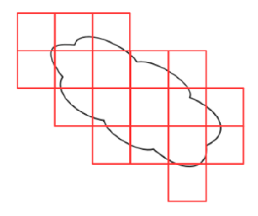
As shown in Figure 2, image objects are irregular polygons, while the inputs of the CNN are regular patches. Thus, patch-based learning must be adapted for analyzing image objects. To resolve this issue, a patch-based strategy was presented for representing an image object as a set of patches, with each patch being a part of the image object. The method of determining the patche representation has great influences on the final classification results. In this study, the center pixel of an image object was considered as the center of the first patch. Then, the patches with fixed sizes were placed to cover the entire image object, and any two patches could not overlap. Therefore, a set of patches were obtained to represent an irregular image object, and then deep features could be extracted from these patches.

2.2. Convolutional Neural Networks

CNN is a multilayer feed-forward neural network commonly composed of convolutional layers, pooling layers, and fully connected layers [14]. The convolutional layers and pooling layers are used to extract deep features from the input image patches, while the fully connected layers are exploited to classify image patches with these deep features. The operations performed in the convolutional layers and the pooling layers can be summarized as:
X l = p o o l p ( f ( X l 1 W l + B l ) )
where the X l 1 denotes the input feature maps of the l t h layer; the W l and the B l denote the weights and biases of convolutional layer, respectively; the f ( · ) represents the nonlinearity function (e.g., sigmoid, tanh, or rectified linear unit (ReLU)); and the p o o l p represents a pooling operation (max pooling or mean pooling) with a kernel size of p . The output feature maps of the l t h layer X l can be obtained through those operations [36].
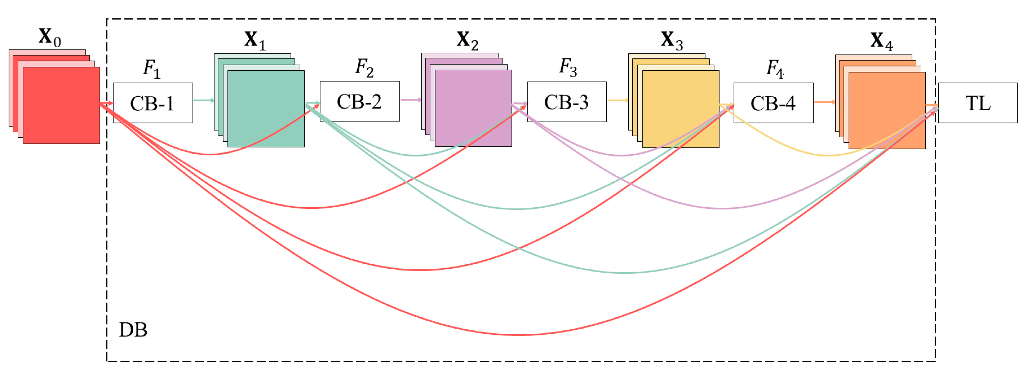
Many CNN models have been proposed in recent years, such as GoogLeNet [37], VGG [38], ResNet [39], and DenseNet [40]. Since DenseNet outperforms the others in deep learning tasks, it was chosen to extract deep features of image objects in this study. DenseNet is mainly composed of dense blocks (DBs) and transition layers (TLs). Each DB further contains several convolutional blocks (CBs). Unlike the other CNN structures, there is a connection between every two CBs in a DB. Consider a DB composed of L CBs. x 0 is the input of the first CB and x l is the output of the l t h CB. F l is a composite function of operations of the l t h CB such as batch normalization (BN), ReLU, pooling, and convolution (Conv.) (Figure 3). The l t h CB receives the feature maps of all preceding CBs, x 0 , , x l 1 , as input (Figure 4):
x l = F l ( [ x 0 , x 1 , , x l 1 ] )
where the operation [ · ] concatenates different feature maps together [40]. Because feature maps with different sizes cannot be concatenated together, a TL (Figure 5) was needed to connect two DBs. The size of feature maps was reduced by the TL due to the pooling operation. Finally, DenseNet (Figure 6) is composed of DBs and TLs alternately connected, whose inputs are image patches and outputs are the classes of center pixels of these image patches, and it was trained through labelled image patches which were obtained from the reference map. Hu et al. [41] demonstrated that the outputs of the last convolutional layer are effective for scene classification. For standardizing deep features, the outputs of BN layer connected after the last convolutional layer were considered as deep features in this paper.

2.3. Deep Feature Aggregation of Image Objects

Through the patches of an image object and the trained CNN model, deep features (the outputs of the last BN layer) of each patch can be learned. The feature map of each patch is composed of m matrices with size s × s . However, these deep features are patch-based, object-based deep features which are needed for classifying image objects. Additionally, the numbers of patches of image objects vary over the sizes and the shapes of image objects. Therefore, different numbers of deep features can be learned for different image objects due to the differences in the number of patches. However, to classify image objects, deep features with identical dimension for all image objects are needed. To resolve this issue, a deep feature aggregation method is proposed in this paper to aggregate the various dimension features of different image objects into identical dimension features for all image objects.
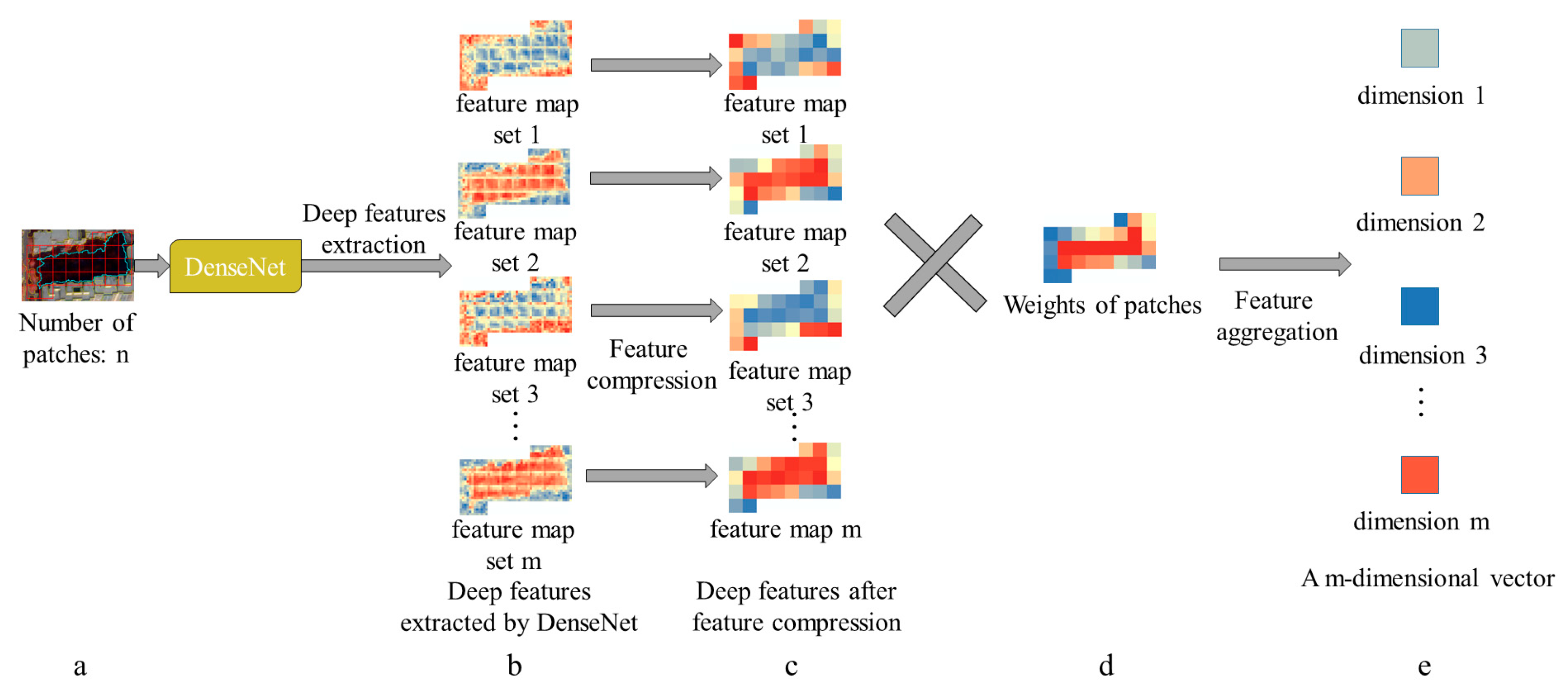
As shown in Figure 7, considering an image object represented by n patches, a total of n × m feature maps with size s × s can be learned, and these feature maps are arranged by their spatial position in Figure 7b. The feature map set 1 in Figure 7b contains the first feature map of all n patches: feature map set 2, feature map set 3, and feature map set m . Since the s × s dimension of each feature map was too high, each feature map needed to be compressed into a single value, so that each feature map set contained n values. In other words, there are n m -dimensional vectors in Figure 7c. The feature compression can be achieved by one of the following operators: mean, variance, maximum, and minimum, for example. The mean operator was used in this paper. To assign these n m -dimensional deep features of patches to one m -dimensional deep features of the image object, an aggregation process needs to be performed. Since in some cases, only parts of patches fall inside an image object, a weighted summation was performed to achieve the aggregation and solve the boundary problem. The weight of each patch was equal to the number of pixels belonging to the image object in the patch divided by the total number of pixels of the image object or the number of pixels of the patch. The result of the aggregation was a m -dimensional vector as shown in Figure 7e. Finally, image objects could be classified with these aggregated features and object features.

2.4. Image Object Classification Using Random Forest Classifier

Random forest (RF) is composed of a multiple classification and regression tree (CART), where each tree is generated using a bootstrap sampling from the input vector and casts a unit vote for the most popular class to classify the input vector [42]. The RF does not overfit because of the Law of Large Numbers and requires two user-defined parameters: the number of trees and the number of random split variables [43]. In [43], it was also demonstrated that once the number of trees reaches a state (100 trees), the number of random split variables only alters the classifier’s accuracy slightly. Additionally, RF is relatively robust to reduce the training set size and noise and can handle categorical data and data with missing values [44]. Therefore, RF was used for image classification in this paper. A m -dimensional deep feature of image objects can be obtained through Section 2.1, Section 2.2, and Section 2.3, and some object features, such as mean values, standard deviations, normalized difference vegetation index (NDVI), shape index, and eight metrics of the gray-level co-occurrence matrix, were also selected for classification. As a result, deep features and object features were concatenated together to train an, RFC and categories of image objects could be obtained (Figure 1, features concatenating and image objects classification).

2.5. Accuracy Assessment

There are lots of methods for the accuracy assessment of remote sensing imagery classification. The Kappa index [45] is widely used in evaluating classification results, but it will introduce problems in calculation and interpretation because the Kappa index is a ratio [46]. In [47], the Bradley–Terry model was used to quantify association in remotely sensed images. In this research, not only the classification results needed to be evaluated, but also the segmentation results needed to be evaluated. Therefore, the segmentation evaluation method proposed in [48] was used; classification results were evaluated by computing the confusion matrix based on the unit of segmentation accuracy assessment.
For segmentation, assume that X = { x i } i = 1 n is a set of n image objects, and Y = { y k } k = 1 m is a set of m reference polygons. For each x X and y Y , if the overlapping degree between x and y is larger than a threshold, x will be regarded as a correspondence of y .
a r e a ( x y ) a r e a ( x ) > 0.5
where a r e a ( x y ) denotes the overlapping area between x and y , the a r e a ( x ) denotes the area of x , and the a r e a ( y ) denotes the area of y . Based on Equation (3), the correspondences between image objects and reference polygons were determined. For an image object x l and its corresponding reference polygon y l , the following three indices can be defined to evaluate their consistent degree [48]:
O S e g l = 1 a r e a ( x l y l ) a r e a ( y l ) U S e g l = 1 a r e a ( x l y l ) a r e a ( x l ) R M S l = O S e g l 2 + U S e g l 2 2
where oversegmentation index O S e g l signifies to what degree reference polygon y l is oversegmented by image object x l ; undersegmentation index U S e g l implies to what degree reference polygon y l is undersegmented by image object x l ; while index R M S l refers to the root mean square. Both O S e g l and U S e g l measure how image object x l fits with its corresponding reference polygon y l , and R M S l integrates these two indices into one single value. O S e g , U S e g , and R M S are the averages of all O S e g l , U S e g l , and R M S l of all objects. The values of O S e g , U S e g , and R M S range from 0 to 1. The smaller the three values, the better the segmentation results; thus, O S e g = 0 , U S e g = 0 , and R M S = 0 signify the best segmentation which was hardly achieved.
For classification, the same as the segmentation, X = { x i } i = 1 n is a set of n image objects, and Y = { y k } k = 1 m is a set of m reference polygons. Considering there are N classes in classification results, and the semantic label of an image object or a reference polygon is c ϵ C = { 1 ,   2 ,   , N } . Therefore, the confusion matrix ( C M ) can be computed as:
C M i C ,   j C = x X   a n d   y Y   a n d   S L ( x ) = = i   a n d   S L ( y ) = = j a r e a ( x y )
where S L ( ) denotes the label of an image object or a reference polygon. Therefore, the overall accuracy ( O A ), producer accuracy ( P A ), and user accuracy ( U A ) were computed as:
O A = i C C M i , i i ϵ C , j ϵ C C M i , j P A i C = C M i , i j C C M j ,   i U A i C = C M i ,   i j C C M i ,   j

3. Datasets and Parameter Settings

3.1. Image Datasets

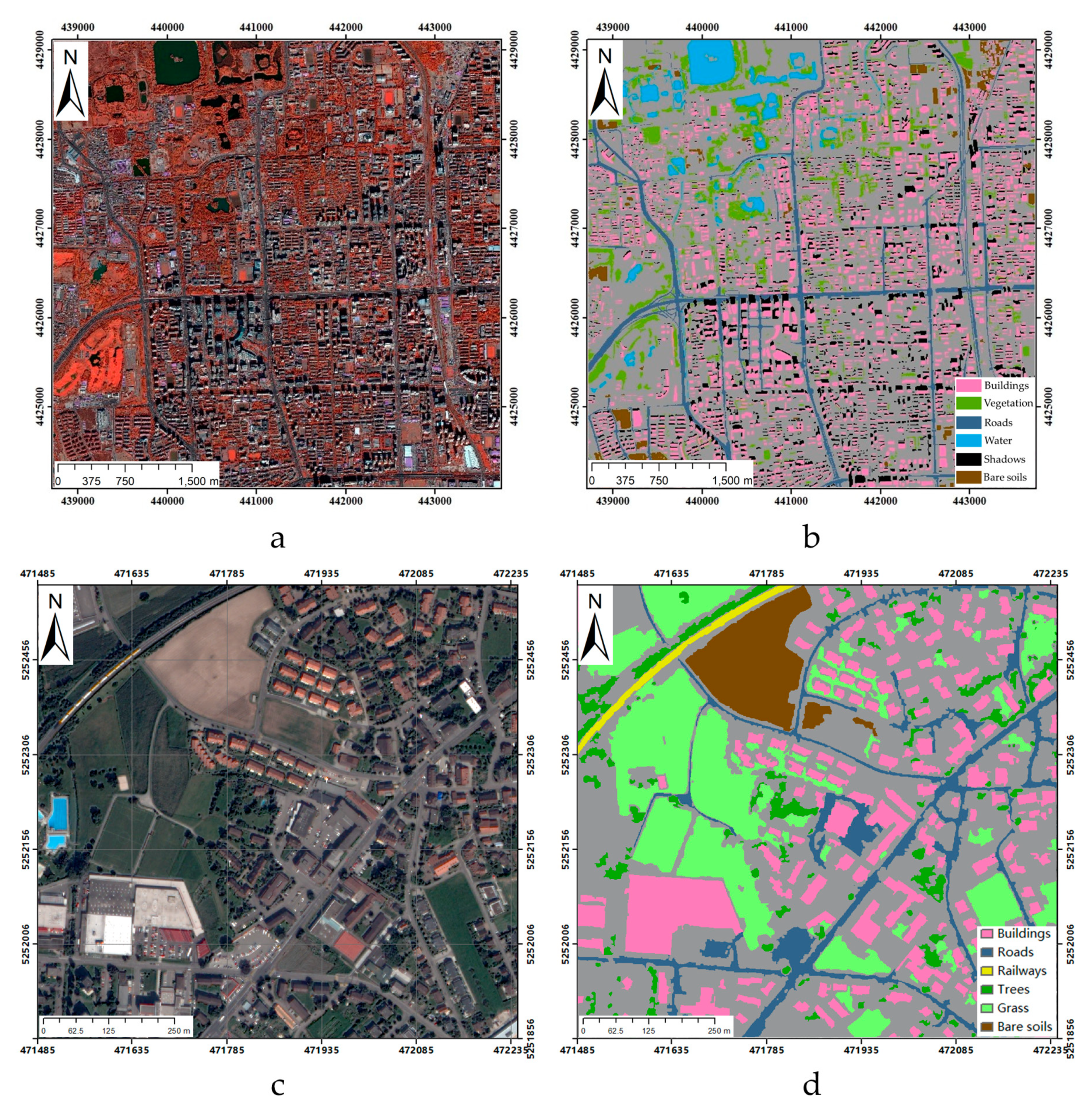
For the experiments, two datasets were used. One was a WorldView-2 imagery of Beijing composed of near infrared, red, green band in 2010 (Figure 8a). The imagery size was 10,000 × 10,000 , and the spatial resolution was 0.5   m . The other one was a QuickBird imagery of Zurich composed of near infrared, red, green, blue band in 2002 (Figure 8c). The imagery size was 1195 × 1264 , and the spatial resolution was 0.6   m .
The image range of Beijing dataset is located between Beijing North Third Ring Road and North Fifth Ring Road. The land cover types in the experimental area include buildings, roads, vegetation, water, and bare soils. Due to the large number of buildings, there are also lots of shadows. Different buildings and roads vary greatly in spectral and spatial structures, which makes it difficult to obtain an accurate land cover map. There are regular residential buildings, irregular commercial buildings, wide and long roads, and narrow and discontinuous residential lanes. Moreover, water and vegetation are mainly distributed in the northwest of the experimental area, and the area of bare soils is the smallest. The reference map was obtained by careful visual interpretation (Figure 8b).
The Zurich dataset [49] is a public dataset, which can be downloaded at https://sites.google.com/site/michelevolpiresearch/data/zurich-dataset. There are 20 chips in the Zurich dataset, and the first chip was used in this paper. Six classes including buildings, roads, railways, trees, grass, and bare soils are presented in the reference map (Figure 8d). Because the image range of the Zurich dataset is small, this dataset is not suitable for parameter analysis and was only used to compare with the state-of-the-art methods.

3.2. Training and Validation Datasets

Due to the inconsistencies between image objects and the inputs of CNN, it is hard to make an end-to-end training for image object classification. The approach proposed in this paper contains two training processes. The first is the CNN training, and the other is the RF training. All training samples were obtained from the reference map.
The training samples for CNN were labelled image patches which were obtained by extending the pixels in the reference map into image patches. For each class, there were 1000 labelled image patches for training and 500 labelled image patches for validation. The 500 labelled image patches were used to validate if the CNN could extract representative features.
RFC was used to classify image objects by considering both deep and object features. The training samples were labelled image objects, and the number of training samples depended on the segmentation scale, which is a parameter of the multiresolution segmentation algorithm. For image objects at a certain segmentation scale, object-based samples were selected based on the reference map. If more than half of the pixels of an image object belonged to one class c , the image object would be assigned to class c as a sample. Finally, approximately four percent of image object samples were selected as training samples of RFC at each segmentation scale.

3.3. Parameter Settings

Segmentation scales determine whether image objects can describe geographic objects exactly. If segmentation scales are too small, geographic objects will be segmented into fragmentary objects, leading to oversegmentation. On the contrary, if segmentation scales are too large, an image object will be related to several geographic objects, leading to undersegmentation. Generally, it is difficult to find a suitable segmentation scale because both over- and undersegmentation always exist simultaneously [50]. Additionally, patch size greatly influences the extraction of deep features. Therefore, nine segmentation scales range from 50 to 210 with an interval of 20 and patch size range from 16 to 64 with an interval of eight were used to explore the influences of segmentation scales on the Beijing dataset. Moreover, to verify the effectiveness of the approach proposed in this paper, comparisons were conducted between our approach with some state-of-the-art methods in both the Beijing dataset and Zurich dataset. For the Beijing dataset, the segmentation scales of all methods are 110, and the patch size of our approach was 48. For the Zurich dataset, the segmentation scales of all methods are 10, and the patch size of our approach was 32. Since seven patch sizes were adopted in the experiments, corresponding to CNN models with seven input sizes, the network structures of CNN in these experiments were the same (Figure 6) except for the input sizes. In this structure, the first DB contained three CBs, the second DB contained six CBs, and the last DB contained four CBs. In the CNN training process, an Adam optimizer was used, and the learning rates, beta1 and beta2, were 0.0001, 0.9, and 0.999, respectively. The batch size was 32. In addition, to prevent overfitting, the method of early stopping was used; that is, if the accuracy of the validation set does not increase for five epochs, then training is stopped. Tensorflow was used in CNN training and deep feature extraction, and scikit-learn was used in image object classification using RFC.

4. Results and Analysis

4.1. Land Cover Classification Results

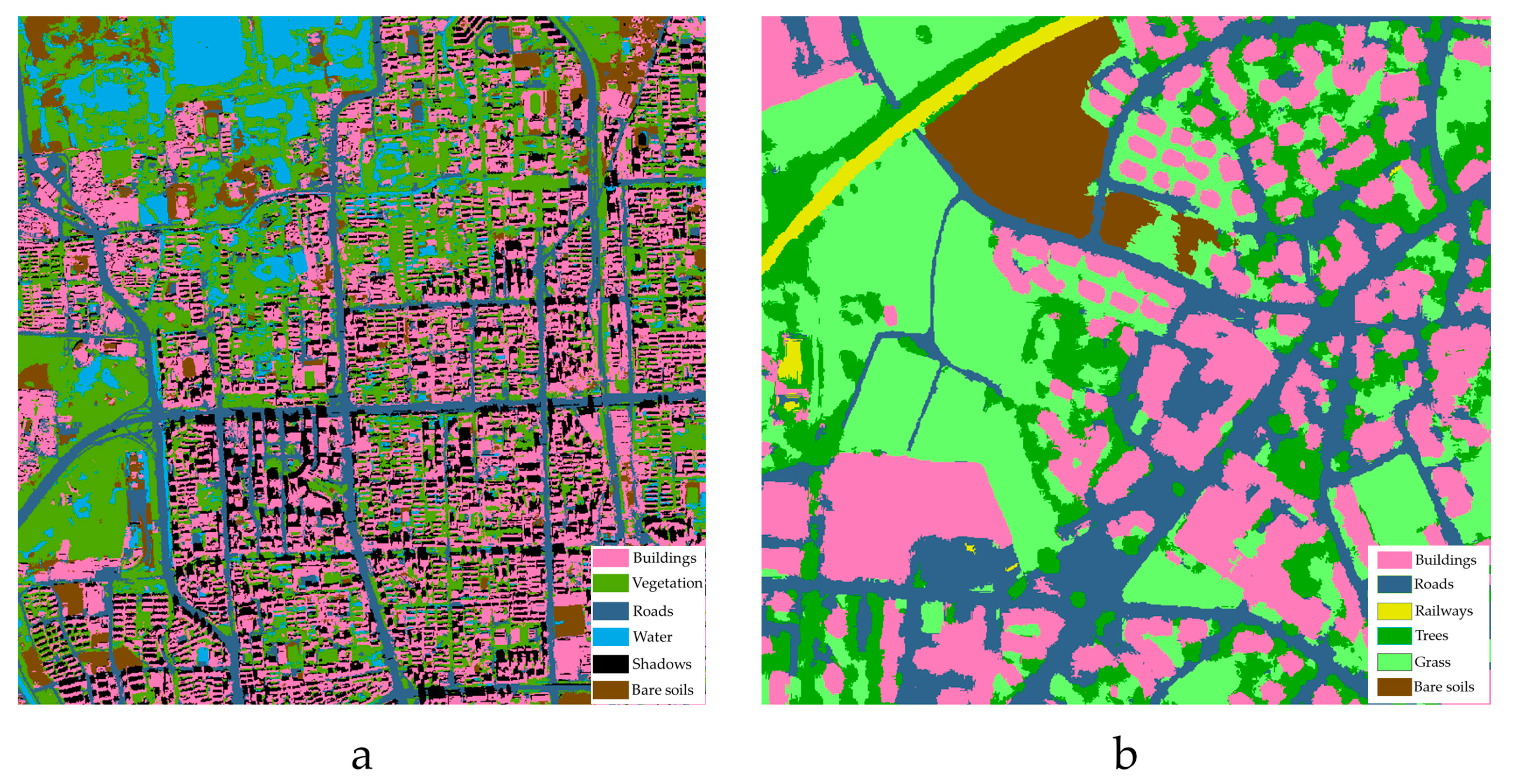
After CNN training, deep feature extraction and aggregation, and RF classification with deep and object features, the classification results of the Beijing dataset and Zurich dataset were obtained and are shown in Figure 9. Table 1 and Table 2 present the P A and the U A of each class in the Beijing dataset and Zurich dataset, respectively.
For the Beijing dataset, the O A was 91.21%, which explains the feasibility of using our method for land cover classification. From the perspective of P A , Water obtained the highest accuracy, and Buildings obtained the lowest accuracy. From the perspective of U A , Buildings obtained the highest accuracy, and Bare soils obtained the lowest accuracy. After comprehensive consideration, Roads obtained the highest classification accuracy, which is also consistent with the classification map.
For the Zurich dataset, the O A was 99.05%. Such a high overall accuracy is mainly because the scene of the Zurich dataset is more single than the Beijing dataset. For example, Buildings in the Beijing dataset are diverse. There are residential buildings, commercial building, schools, and museums in the Beijing dataset. On the contrary, buildings are mainly residential buildings in the Zurich dataset. From the perspective of P A and U A , Bare soils obtained the highest classification accuracy, and Trees obtained the lowest classification accuracy.
To further explore the uncertainty of our method, 5-fold stratified cross validations were performed 50 times in RF classification with deep and object features. The box plots of classification accuracies are shown in Figure 10. It can be seen from Figure 10a,c that the range of overall accuracies of the Beijing dataset and Zurich dataset was very small, which demonstrates that overall accuracy is less affected by the random selection of samples. Therefore, our method is quite robust for different samples. For the Beijing dataset (Figure 10b), the producer accuracies of Buildings, Vegetation, and Shadows were higher than Roads, Water, and Bare soils. At the same time, the range of producer accuracy of Buildings. Vegetation and Shadows are lower than Roads, Water and Bare soils. For Zurich dataset (Figure 10d), Trees gets the lowest producer accuracy and get the highest range of producer accuracy.

4.2. Influences of Segmentation Scales

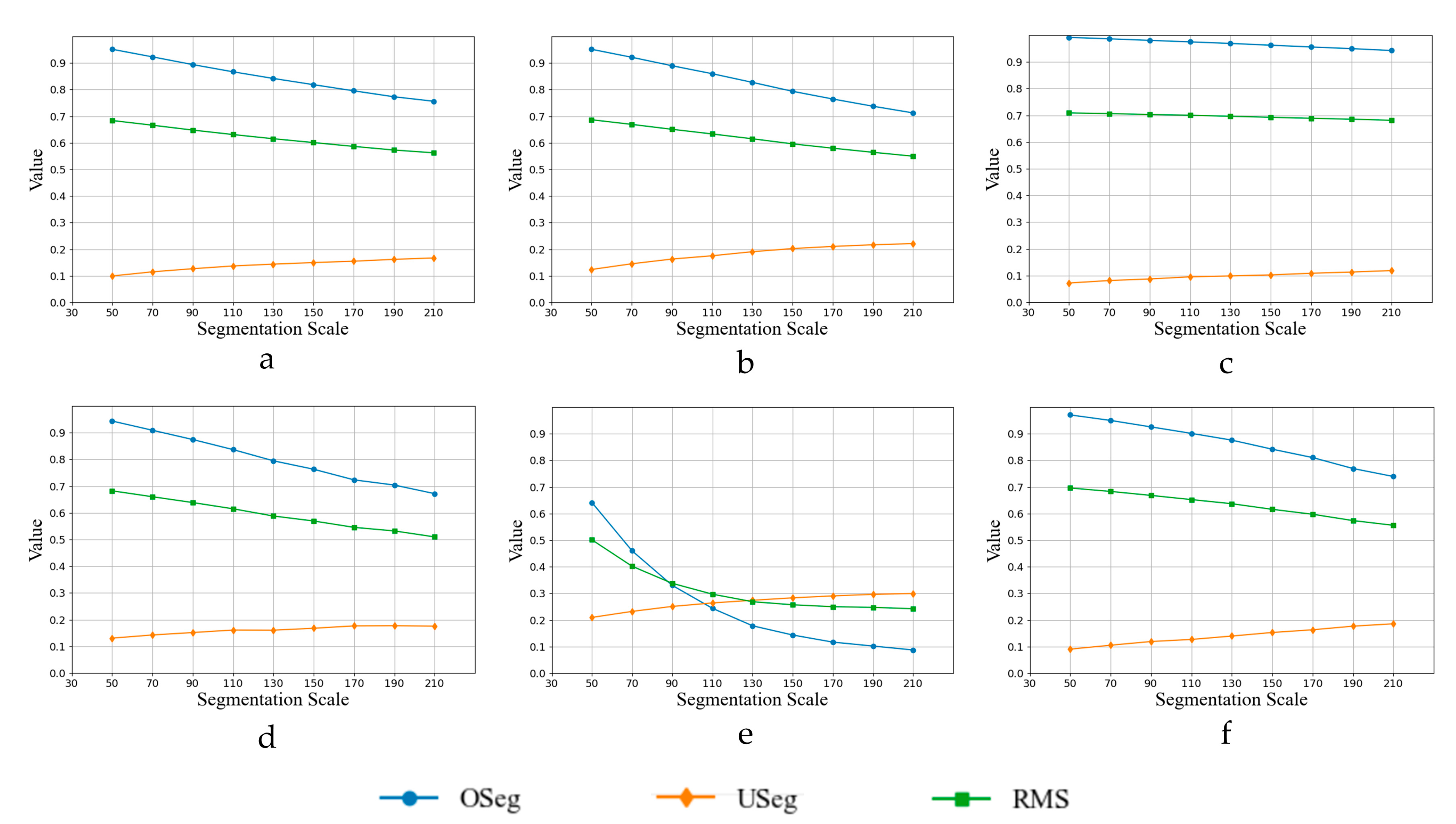
Nine segmentation scales were used to explore the influences of segmentation scales on the Beijing dataset in this section. Indices O S e g , U S e g , and R M S of different ground entities at different scales are shown in Figure 11. When segmentation scales became larger, the values of indices O S e g and R M S of all ground entities became smaller, while the values of U S e g became larger. At the segmentation scale of 210, the values of O S e g were still much higher than that of U S e g for all ground entities except for shadows, meaning that these ground entities were still oversegmented. Buildings were also oversegmented because buildings with windows and roofs were heterogeneous; vegetation was oversegmented because their distribution were uneven: some places are dense, while some are sparse. Bare soils were also heterogeneous. Only shadows were relatively homogeneous; thus, the oversegmentation phenomenon was not significant. This means that a larger segmentation scale should be utilized to segment shadows. However, the conclusion may be different from the perspective of classification results.
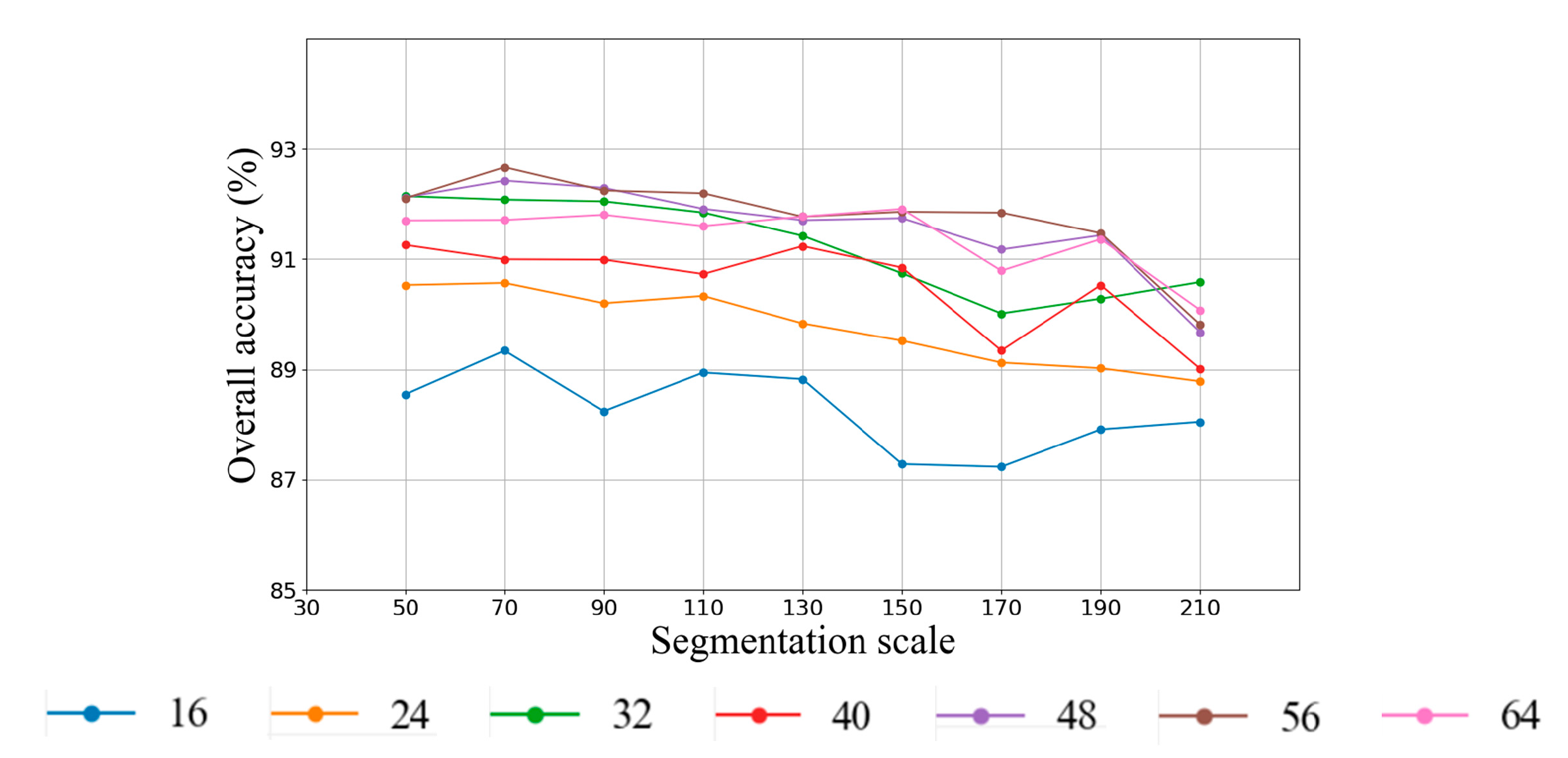
For image objects generated by the above nine segmentation scales, the proposed approach was used for classification. The overall classification accuracies varied over segmentation scales (Figure 12), and so do the producer accuracies of different classes (Figure 13). As segmentation scales become larger, the overall accuracies remain unchanged first, and then decrease slightly. There were similar trends for different ground entities. Therefore, a smaller segmentation scale should be used to generate image objects in terms of classification results. This was exactly the opposite conclusion to the segmentation evaluation results.
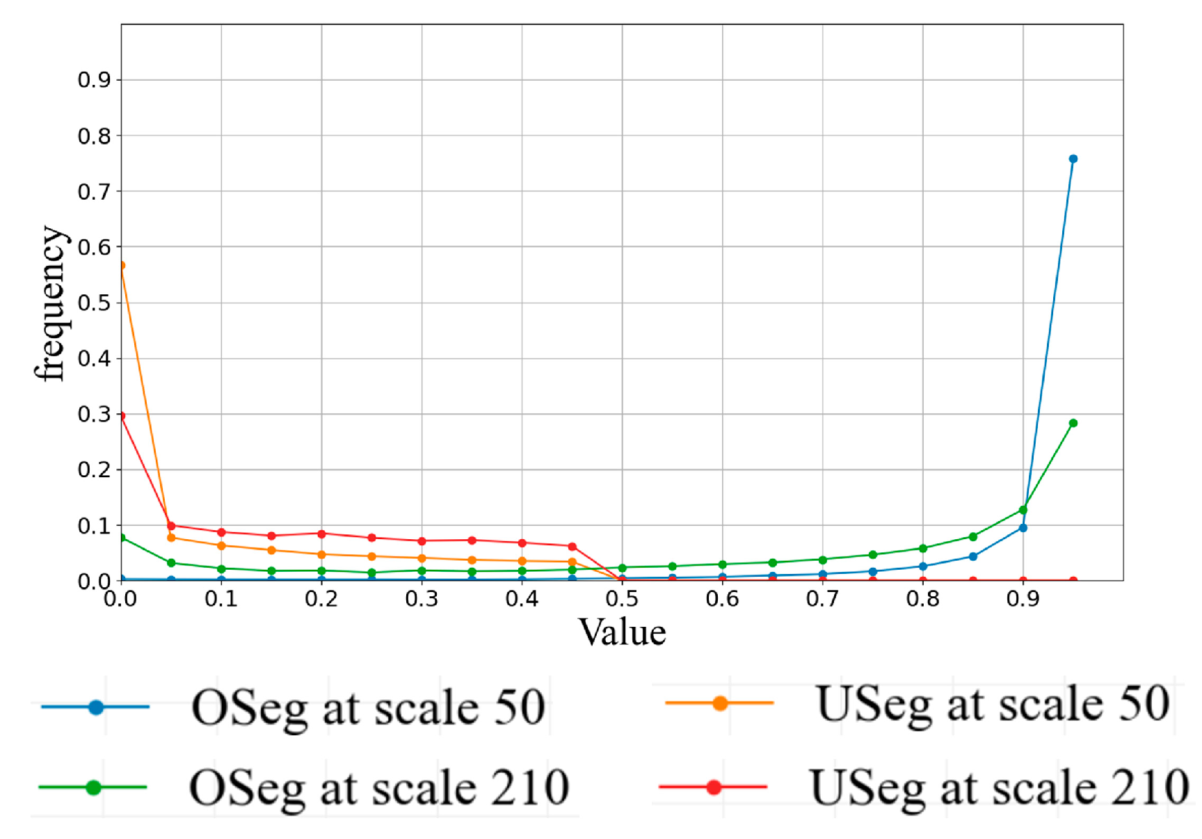
To explore the reasons for the segmentation scale selection, Figure 14 shows the frequency distribution histograms of O S e g l and U S e g l at the two segmentation scales of 50 and 210. Apparently, when the segmentation scale was 50, over 90% image objects had O S e g values greater than 0.8, while less than 1% image objects had U S e g values greater than 0.5. That is, most image objects were oversegmented at the scale 50. When the segmentation scale was 210, both the over- and undersegmentation coexisted. However, how do over- and undersegmentation impact classification? As shown in Figure 15, A–G represent geographic objects with different categories, a-f represent oversegmented image objects of G, and g represents undersegmented image objects of G. For oversegmented image objects a-f, whether they were classified correctly or not, they affected the classification results of adjacent geographic objects A–F slightly. However, for undersegmented image object g, it was mixed by diverse classes of pixels. If g was classified correctly, the pixels of adjacent geographic objects A–F would be misclassified, because A–F are different categories with G. If g was misclassified, geographic object G would be misclassified, too. Therefore, whether undersegmented image objects are classified correctly or not will lead to incorrect classification results. All in all, if the segmentation cannot completely coincide with image objects and geographic objects, a smaller segmentation scale is recommended in this paper, but the scale should not be too small; otherwise, the phenomenon of the “salt and pepper effect” will occur.

4.3. Influences of Patch Sizes on Classification

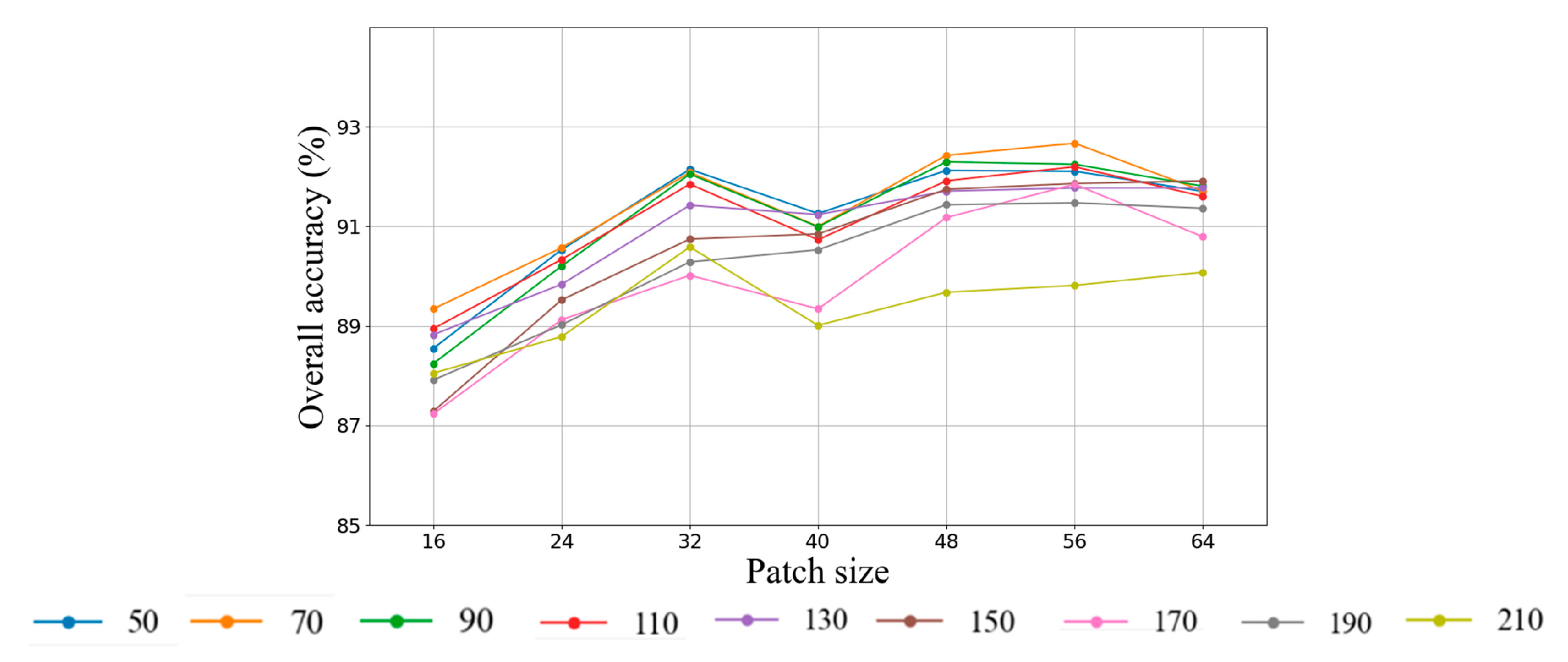
The unit of patch size was pixel, and it greatly influenced the extraction of deep features. To explore how patch size affects deep feature extraction, seven patch sizes were chosen. Figure 16 shows the variation of overall accuracies over patch sizes, while Figure 17 illustrates that of the producer accuracies over patch sizes. In Figure 16, overall accuracies increased firstly and decreased lastly, and the overall accuracy reached its highest when the patch size was close to 48. Additionally, in Figure 17, buildings were most sensitive to the change of patch sizes, while the producer accuracies of other ground entities changed slightly with the change of patch sizes.
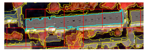
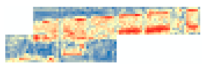
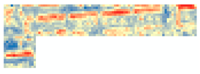
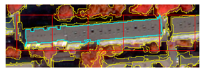
To explore the influence of patch sizes on deep feature extraction, an image object of building class was chosen as an example to illustrate the patch representation and deep feature extraction, because buildings are most sensitive to the change of patch size (Table 3). Results show that when patch size was relatively small or relatively large, the outlines of buildings in deep features were not obvious; but when patch size was 48, the outline of the building in deep features was obvious and the classification accuracy was the highest, simultaneously. Therefore, it is important to choose an appropriate patch size, which is related to the data resolution, sizes of image objects, and the method to place the patch. The appropriate patch size in this paper was 48.

5. Discussion

5.1. Object Features vs. Deep Features

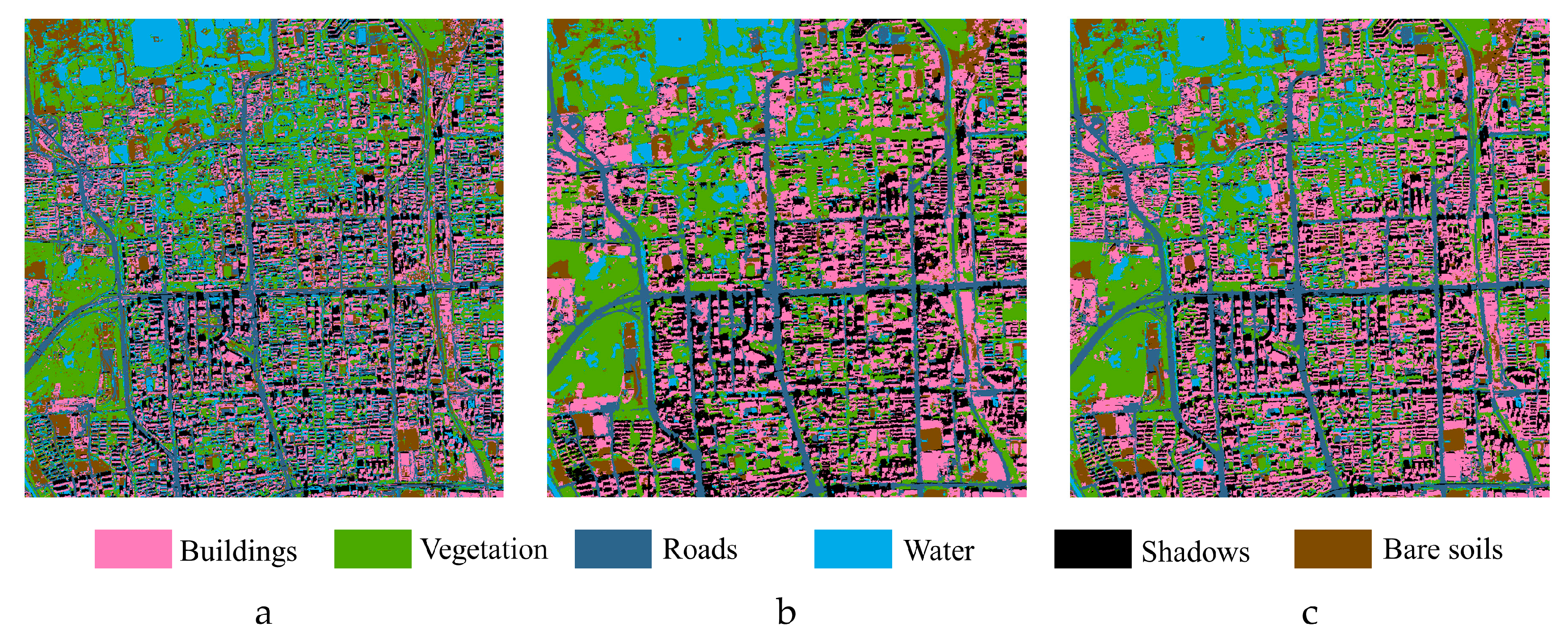
Both deep and object features can be used to classify VHR images, but which one is more important for classification? A comparative experiment composed of three different features combinations was designed to answer this question in the Beijing dataset. The first experiment explored the effectiveness of object features on classification; the second explored the effectiveness of deep features; while the third considered both object and deep features. The classification results are shown in Figure 18. The largest difference between the first and the second experiments relied on the results of roads and buildings. The differences between the latter two experiments appeared to be small.
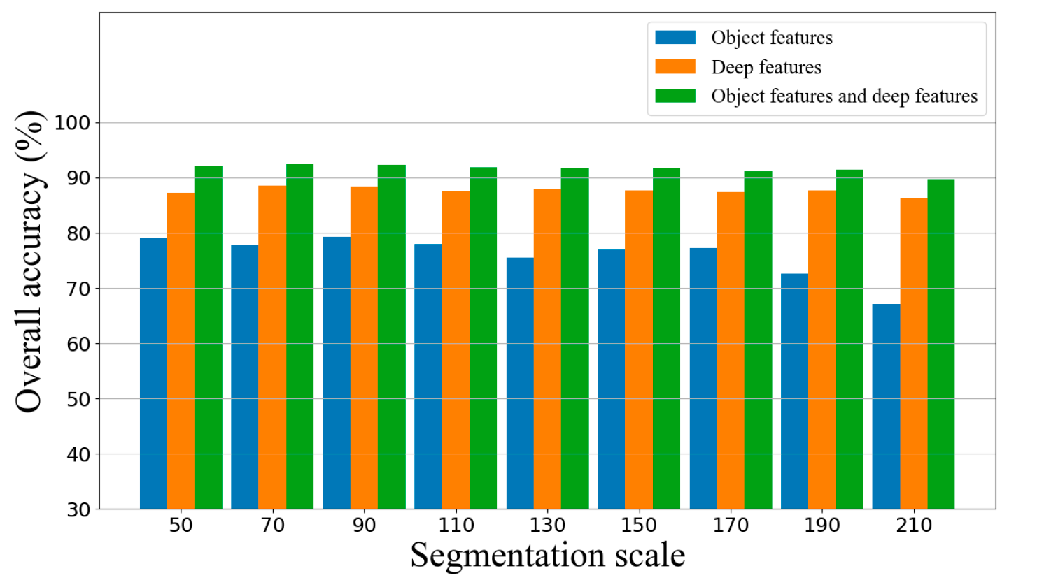
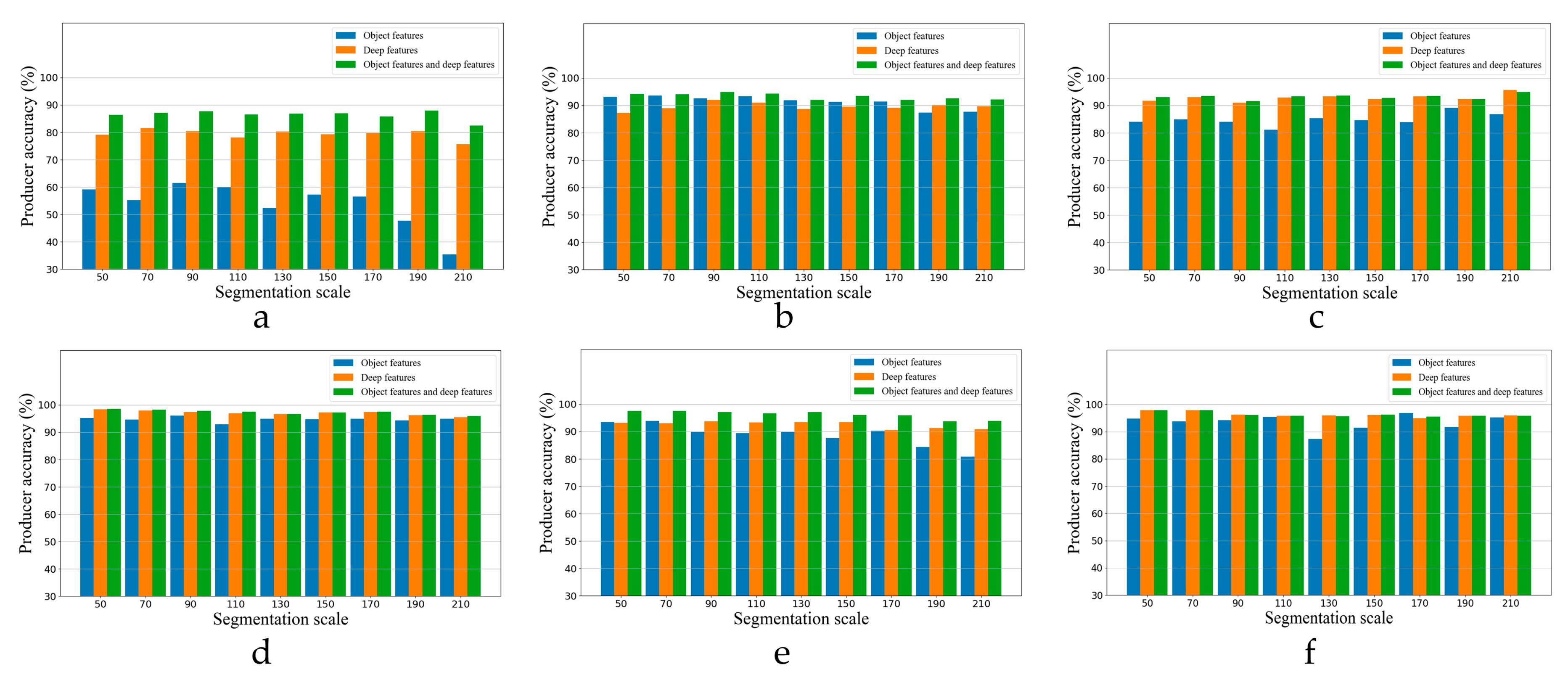
The overall accuracies of the three experiments are shown in Figure 19, and the producer accuracies are shown in Figure 20. From the perspective of overall accuracy, no matter which segmentation scale was used, the classification result with both object and deep features produced the highest classification accuracy, while classification result with object features led to the lowest accuracy. Therefore, deep features are more important than object features to classify VHR images, although object features are also essential in general. At the same time, the conclusion is not always correct for all ground entities. Most ground entities are in line with the above conclusion, but for vegetation and shadows at smaller scales, object features can produce better classification results than deep features. This is because image objects are relatively homogeneous at a small scale, while NDVI and spectral mean values can distinguish vegetation and shadows well from other ground entities, respectively. The larger the segmentation scales become, the more complicated image objects are, and the more robust features are needed. Additionally, in Figure 19, the effects of segmentation scales on overall accuracies of the experiments two and three were much lower than the impacts on the overall accuracies of the first experiment. In other words, deep features can reduce the impact of segmentation scales on classification results. Therefore, it is recommended that both deep and object features should be considered in classification.

5.2. The Importance of Deep Feature Aggregation

Deep feature aggregation is an important operator in our approach. Classification results can be also obtained without deep feature aggregation. For example, deep features of patches can be used to classify these patches and a decision-level fusion through patches-based voting can be performed to obtain the classification results of image objects. However, many useful spectral features such as NDVI cannot be accurately learned through CNN. In addition, deep and object features are obtained through different units. That is, deep features are related to patches, while object features are concerned with image objects. Therefore, to combine these two types of features, aggregating patch-based deep features to object-based deep features is necessary.
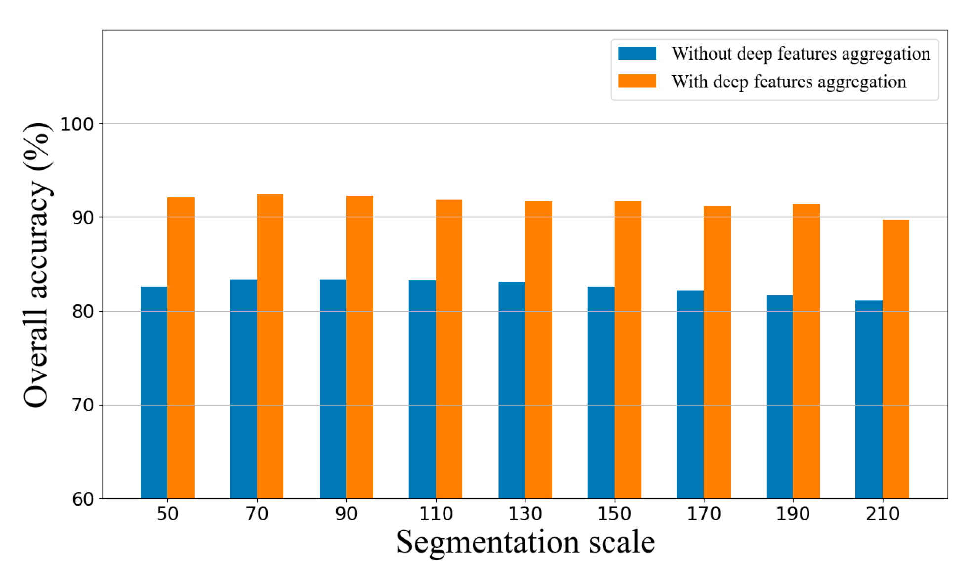
To verify the importance of deep feature aggregation, deep features of patches are used to classify these patches and a decision-level fusion by patches-based voting is performed to obtain the classification results of image objects without deep feature aggregation on Beijing dataset. The patch size is 48 in this experiment. As shown in Figure 21, larger classification accuracy is obtained with deep feature aggregation whether which scale is selected. Additionally, compared with Figure 19, it can be found that deep features and deep feature aggregation can produce larger classification accuracy than deep features alone. Therefore, deep feature aggregation is important.

5.3. Comparison with the State-Of-The-Art Methods

There are three main object-based CNN methods [32,33,34] in current literature. How does the proposed approach differ from these existing methods? Which method can produce the best classification result for VHR imagery? The main differences between the proposed approach and those existing methods are summarized as follows:
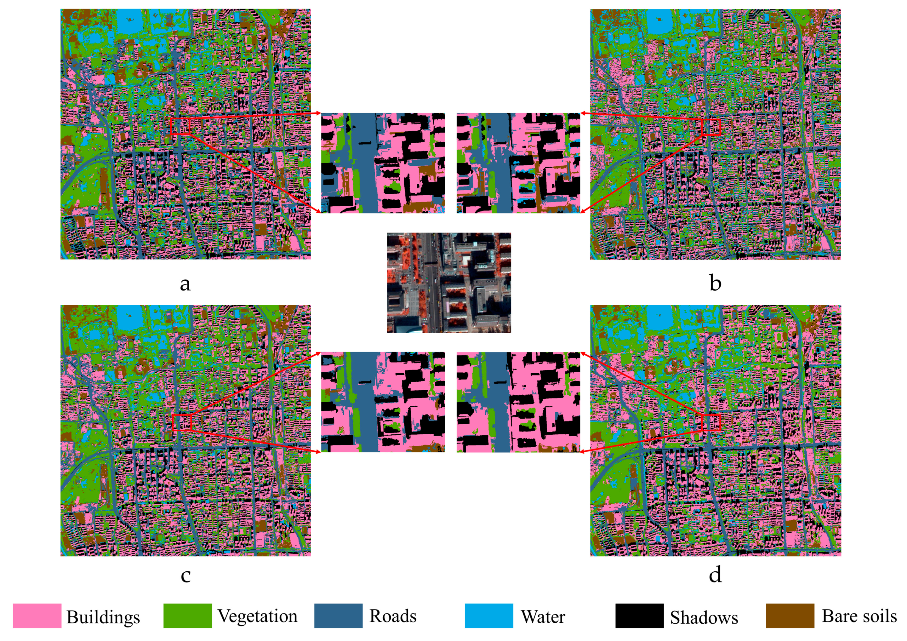
(1) Different methods to place patches. Different methods adopt different strategies to place patches. As shown in Figure 22a, Fu et al. [34] applied only one patch to one image object. The center of the patch was located at the center of the image object. However, for linearly shaped image objects, this method may be inappropriate to place patches. Zhao et al. [32] placed one patch on each pixel of an image object (Figure 22b). However, the patches were too dense and overlapped largely, leading to extremely massive computation and a large correlation among neighboring pixels. Zhang et al. [33] divided image objects into two types: general image objects and linearly shaped image objects. Large patches were used for general image objects, while several small patches were adopted for linearly shaped image objects. The positions of patches were determined by convolutional position analysis. For a general image object, the method to place patches is similar to Figure 22a. For a linearly shaped image object, the method to place patches is shown in Figure 22c. However, in this way, the patches cannot represent image objects exactly and take advantage of all the information. In our method, a set of patches was used to represent an image object, and all patches covered the entire object together (Figure 22d). The number of patches for an image object was determined by patch sizes and the shape of the image object. Compared with the former three methods, deep features of different patches were weighted, and deep features of image objects were obtained through deep feature aggregation in our method.
(2) Different methods to obtain object class from patches. Different deep features can be learned from different patches of an image object; that is, deep features are patch-based. As a result, an aggregation operator is needed to aggregate these deep features to classify image objects or to generate a fixed dimension feature for further classification. Fu et al. [34] utilized only one patch to represent an image object; thus, no aggregation operator is used. Zhao et al. [32] and Zhang et al. [33] utilized the majority voting operator to obtain classification results from these patch-based deep features. In other words, Zhao et al. and Zhang et al. used a decision-level fusion, and a feature-level fusion was used in this paper.
(3) Different roles of object and deep features playing in classification. As demonstrated in Section 5.1, although deep features can help to classify image objects directly, they cannot completely replace object features, including spectral, shape, texture, and other features. Existing work [33,34] only considered deep features and ignored object features. Zhao et al. [32] combined object features with the deep features of pixels to classify pixels. Unfortunately, both object and deep features were extracted from different units: object features from image objects, while deep features from pixels. As a result, it is hard to combine the two kinds of features. However, this study resolved this issue by aggregating deep features of patches into deep features of objects through mean and weighted sum operators. Finally, deep and object features of image objects were concatenated together to classify image objects.
The classification results of the four methods on Beijing dataset and Zurich dataset are shown in Figure 23 and Figure 24, their classification accuracies are reported in Table 4 and Table 5. These two tables demonstrate that our method can obtain the best classification accuracy. For Beijing dataset, the main advantage was that better classification results of buildings and water for our method, while the misclassification of buildings and water by other three methods was more significant. Buildings and roads, water, and shadows are more likely to be confused in the other three methods while they were very well classified in our method. For the Zurich dataset, whether from the perspective of PA or from the perspective of UA, our method can obtain very good results for each class. At the same time, the other three methods cannot achieve good results for every class. Therefore, compared with the three existing object-based CNN methods, our method has more advantages for the classification of VHR imagery.

5.4. Limitations and Future Work

A novel method was proposed to integrate deep features into the GEOBIA paradigm in this study and was used for VHR imagery classification. Although the proposed method can achieve better classification results than existing object-based CNN methods, there were still some limitations.
The first is the determination of the method of patch division and the selection of patch size. The results of deep feature extraction depend on patch sizes and the method of patch division. For simplicity, this paper adopted the fixed patch size. However, different ground entities may vary in sizes and structures; thus, different patch sizes should be considered. As a result, adaptive patch sizes will be addressed in future.
The second is the method of aggregating deep features, which directly affects how the deep features extracted through patches are aggregated into image objects with less information loss. The mean operator was used to compress the deep features of each patch, and weighted summation was used to aggregate deep features extracted from different patches in this paper. However, the mean function may lose some information, and the weighted summation may not be the best way to aggregate deep features of different patches. Therefore, other methods of deep feature aggregation will be the focus of future work.

6. Conclusions

In this study, we showed an effective method of integrating deep features into GEOBIA for VHR remote sensing imagery classification. We proposed a patch-based approach for representing image objects using patches and learning patch-based deep features and a deep feature aggregation method for aggregating patch-based deep features into object-based deep features, in order to extract deep features from irregular image objects through CNN. Results show that smaller segmentation scales were more conducive to VHR remote sensing imagery classification, and it was not appropriate to select too large or too small patches, as the patch size should be determined by imagery and its resolution. Moreover, we performed 5-fold stratified cross validations 50 times to demonstrate the stability of our method. Additionally, we found that although deep features are better than object features for classification in most cases, object features still matter for improving classification results. We demonstrated the deep feature aggregation is a critical step in our method. In the comparison with existing object-based CNN methods, our method achieved the highest overall accuracies, and the overall accuracies were 91.21% for the Beijing dataset and 99.05% for the Zurich dataset. Therefore, the method presented in this paper has great application prospects in LULC mapping.
Though our method achieves better classification results than the state-of-the-art methods, there still are some points that can be improved. The compression method with less information lost can be developed, and other methods of deep feature aggregation can be used. A better classification result can be achieved through these methods.

Author Contributions

Funding acquisition, S.D. (Shihong Du); investigation, B.L.; methodology, B.L., S.D. (Shihong Du), S.D. (Shouji Du) and X.Z.; supervision, S.D. (Shihong Du); visualization, B.L.; writing—original draft, B.L.; writing—review and editing, S.D. (Shihong Du). All authors have read and agreed to the published version of the manuscript.

Funding

This research was funded by the National Natural Science Foundation of China, grant number 41871372.

Conflicts of Interest

There is no conflict of interest.

References

  1. Martinez, S.; Mollicone, D. From Land Cover to Land Use: A Methodology to Assess Land Use from Remote Sensing Data. Remote Sens. 2012, 4, 1024–1045. [Google Scholar] [CrossRef] [Green Version]
  2. Pesaresi, M.; Guo, H.D.; Blaes, X.; Ehrlich, D.; Ferri, S.; Gueguen, L.; Halkia, M.; Kauffmann, M.; Kemper, T.; Lu, L.L.; et al. A Global Human Settlement Layer from Pptical HR/VHR RS Data: Concept and First Results. IEEE J. Sel. Top. Appl. Earth Observ. Remote Sens. 2013, 6, 2102–2131. [Google Scholar] [CrossRef]
  3. Zhang, L.P.; Huang, X.; Huang, B.; Li, P.X. A Pixel Shape Index Coupled with Spectral Information for Classification of High Spatial Resolution Remotely Sensed Imagery. IEEE Trans. Geosci. Remote Sens. 2006, 44, 2950–2961. [Google Scholar] [CrossRef]
  4. Huang, X.; Zhang, L.P.; Li, P.X. Classification and Extraction of Spatial Features in Urban Areas Using High-Resolution Multispectral Imagery. IEEE Geosci. Remote Sens. Lett. 2007, 4, 260–264. [Google Scholar] [CrossRef]
  5. Blaschke, T. Object based image analysis for remote sensing. ISPRS J. Photogramm. Remote Sens. 2010, 65, 2–16. [Google Scholar] [CrossRef] [Green Version]
  6. Blaschke, T.; Hay, G.J.; Kelly, M.; Lang, S.; Hofmann, P.; Addink, E.; Feitosa, R.Q.; van der Meer, F.; van der Werff, H.; van Coillie, F.; et al. Geographic Object-Based Image Analysis—Towards a new paradigm. ISPRS J. Photogramm. Remote Sens. 2014, 87, 180–191. [Google Scholar] [CrossRef] [Green Version]
  7. Ma, L.; Cheng, L.; Li, M.C.; Liu, Y.X.; Ma, X.X. Training set size, scale, and features in Geographic Object-Based Image Analysis of very high resolution unmanned aerial vehicle imagery. ISPRS J. Photogramm. Remote Sens. 2015, 102, 14–27. [Google Scholar] [CrossRef]
  8. Du, S.H.; Zhang, F.L.; Zhang, X.Y. Semantic classification of urban buildings combining VHR image and GIS data: An improved random forest approach. ISPRS J. Photogramm. Remote Sens. 2015, 105, 107–119. [Google Scholar] [CrossRef]
  9. Griffith, D.C.; Hay, G.J. Integrating GEOBIA, Machine Learning, and Volunteered Geographic Information to Map Vegetation over Rooftops. ISPRS Int. Geo-Inf. 2018, 7, 462. [Google Scholar] [CrossRef] [Green Version]
  10. De Luca, G.; Silva, J.M.N.; Cerasoli, S.; Araujo, J.; Campos, J.; Di Fzaio, S.; Modica, G. Object-Based Land Cover Classification of Cork Oak Woodlands Using UAV Imagery and Orfeo ToolBox. Remote Sens. 2019, 11, 1238. [Google Scholar] [CrossRef] [Green Version]
  11. Ribeiro, F.F.; Roberts, D.A.; Hess, L.L.; Davis, F.W.; Caylor, K.K.; Daldegan, G.A. Geographic Object-Based Image Analysis Framework for Mapping Vegetation Physiognomic Types at Fine Scales in Neotropical Savannas. Remote Sens. 2020, 12, 1721. [Google Scholar] [CrossRef]
  12. Zhang, F.; Du, B.; Zhang, L.P.; Xu, M.Z. Weakly Supervised Learning Based on Coupled Convolutional Neural Networks for Aircraft Detection. IEEE Trans. Geosci. Remote Sens. 2016, 54, 5553–5563. [Google Scholar] [CrossRef]
  13. LeCun, Y.; Boser, B.; Denker, J.S.; Henderson, D.; Howard, R.E.; Hubbard, W.; Jackel, L.D. Backpropagation Applied to Handwritten Zip Code Recognition. Neural Comput. 1989, 1, 541–551. [Google Scholar] [CrossRef]
  14. Krizhevsky, A.; Sutskever, I.; Hinton, G.E. ImageNet classification with deep convolutional neural networks. Commun. ACM 2017, 60, 84–90. [Google Scholar] [CrossRef]
  15. Chen, Y.S.; Jiang, H.L.; Li, C.Y.; Jia, X.P.; Ghamisi, P. Deep Feature Extraction and Classification of Hyperspectral Images Based on Convolutional Neural Networks. IEEE Trans. Geosci. Remote Sens. 2016, 54, 6232–6251. [Google Scholar] [CrossRef] [Green Version]
  16. Chen, X.Y.; Xiang, S.M.; Liu, C.L.; Pan, C.H. Vehicle Detection in Satellite Images by Hybrid Deep Convolutional Neural Networks. IEEE Geosci. Remote Sens. Lett. 2014, 11, 1797–1801. [Google Scholar] [CrossRef]
  17. Ren, S.Q.; He, K.M.; Girshick, R.; Sun, J. Faster R-CNN: Towards Real-Time Object Detection with Region Proposal Networks. IEEE Trans. Pattern Anal. Mach. Intell. 2017, 39, 1137–1149. [Google Scholar] [CrossRef] [Green Version]
  18. Chen, Z.; Zhang, T.; Ouyang, C. End-to-End Airplane Detection Using Transfer Learning in Remote Sensing Images. Remote Sens. 2018, 10, 139. [Google Scholar] [CrossRef] [Green Version]
  19. Ghorbanzadeh, O.; Meena, S.R.; Blaschke, T.; Aryal, J. UAV-Based Slope Failure Detection Using Deep-Learning Convolutional Neural Networks. Remote Sens. 2019, 11, 2046. [Google Scholar] [CrossRef] [Green Version]
  20. Liu, Y.F.; Zhong, Y.F.; Qin, Q.Q. Scene Classification Based on Multiscale Convolutional Neural Network. IEEE Trans. Geosci. Remote Sens. 2018, 56, 7109–7121. [Google Scholar] [CrossRef] [Green Version]
  21. De Lima, R.P.; Marfurt, K. Convolutional Neural Network for Remote-Sensing Scene Classification: Transfer Learning Analysis. Remote Sens. 2020, 12, 86. [Google Scholar] [CrossRef] [Green Version]
  22. Shelhamer, E.; Long, J.; Darrell, T. Fully Convolutional Networks for Semantic Segmentation. IEEE Trans. Pattern Anal. Mach. Intell. 2017, 39, 640–651. [Google Scholar] [CrossRef] [PubMed]
  23. Zhao, W.Z.; Du, S.H.; Wang, Q.; Emery, W.J. Contextually guided very-high-resolution imagery classification with semantic segments. ISPRS-J. Photogramm. Remote Sens. 2017, 132, 48–60. [Google Scholar] [CrossRef]
  24. Yang, M.D.; Tseng, H.H.; Hsu, Y.C.; Tsai, H.P. Semantic Segmentation Using Deep Learning with Vegetation Indices for Rice Lodging Identification in Multi-date UAV Visible Images. Remote Sens. 2020, 12, 633. [Google Scholar] [CrossRef] [Green Version]
  25. Abdi, O. Climate-Triggered Insect Defoliators and Forest Fires Using Multitemporal Landsat and TerraClimate Data in NE Iran: An Application of GEOBIA TreeNet and Panel Data Analysis. Sensors 2019, 19, 3965. [Google Scholar] [CrossRef] [Green Version]
  26. Feng, F.; Wang, S.T.; Wang, C.Y.; Zhang, J. Learning Deep Hierarchical Spatial-Spectral Features for Hyperspectral Image Classification Based on Residual 3D-2D CNN. Sensors 2019, 19, 5276. [Google Scholar] [CrossRef] [Green Version]
  27. Liu, B.; Yu, X.C.; Zhang, P.Q.; Yu, A.Z.; Fu, Q.Y.; Wei, X.P. Supervised Deep Feature Extraction for Hyperspectral Image Classification. IEEE Trans. Geosci. Remote Sens. 2018, 56, 1909–1921. [Google Scholar] [CrossRef]
  28. Zhao, W.Z.; Du, S.H.; Emery, W.J. Object-Based Convolutional Neural Network for High-Resolution Imagery Classification. IEEE J. Sel. Top. Appl. Earth Observ. Remote Sens. 2017, 10, 3386–3396. [Google Scholar] [CrossRef]
  29. Liu, T.; Abd-Elrahman, A. An Object-Based Image Analysis Method for Enhancing Classification of Land Covers Using Fully Convolutional Networks and Multi-View Images of Small Unmanned Aerial System. Remote Sens. 2018, 10, 457. [Google Scholar] [CrossRef] [Green Version]
  30. Liu, T.; Abd-Elrahman, A.; Morton, J.; Wilhelm, V.L. Comparing Fully Convolutional Networks, Random Forest, Support Vector Machine, and Patch-Based Deep Convolutional Neural Networks for Object-Based Wetland Mapping Using Images from Small Unmanned Aircraft System. GISci. Remote Sens. 2018, 55, 243–264. [Google Scholar] [CrossRef]
  31. Mboga, N.; Georganos, S.; Grippa, T.; Lennert, M.; Vanhuysse, S.; Wolff, E. Fully Convolutional Networks and Geographic Object-Based Image Analysis for the Classification of VHR Imagery. Remote Sens. 2019, 11, 597. [Google Scholar] [CrossRef] [Green Version]
  32. Langkvist, M.; Kiselev, A.; Alirezaie, M.; Loutfi, A. Classification and Segmentation of Satellite Orthoimagery Using Convolutional Neural Networks. Remote Sens. 2016, 8, 329. [Google Scholar] [CrossRef] [Green Version]
  33. Zhang, C.; Sargent, I.; Pan, X.; Li, H.P.; Gardiner, A.; Hare, J.; Atitinson, P.M. An object-based convolutional neural network (OCNN) for urban land use classification. Remote Sens. Environ. 2018, 216, 57–70. [Google Scholar] [CrossRef] [Green Version]
  34. Fu, T.Y.; Ma, L.; Li, M.C.; Johnson, B.A. Using convolutional neural network to identify irregular segmentation objects from very high-resolution remote sensing imagery. J. Appl. Remote Sens. 2018, 12, 025010. [Google Scholar] [CrossRef]
  35. Baatz, M.; Schape, A. Multiresolution Segmentation: An Optimization Approach for High Quality Multi-Scale Image Segmentation. In Angewandte Geographische Informations-Verarbeitung, XII; Strobl, J., Ed.; Wichmann Verlag: Karlsruhe, Germany; Berlin, Germany, 2000; Volume 58, pp. 12–23. [Google Scholar]
  36. Lee, H.; Kwon, H. Going Deeper With Contextual CNN for Hyperspectral Image Classification. IEEE Trans. Image Process. 2017, 26, 4843–4855. [Google Scholar] [CrossRef] [Green Version]
  37. Szegedy, C.; Liu, W.; Jia, Y.Q.; Sermanet, P.; Reed, S.; Anguelov, D.; Erhan, D.; Vanhoucke, V.; Rabinovich, A. Going Deeper with Convolutions. In Proceedings of the IEEE Conference on Computer Vision and Pattern Recognition, Boston, MA, USA, 7–12 June 2015. [Google Scholar]
  38. Simonyan, K.; Zisserman, A. Very Deep Convolutional Networks for Large-Scale Image Recognition. arXiv 2014, arXiv:1409.1556. [Google Scholar]
  39. He, K.M.; Zhang, X.Y.; Ren, S.Q.; Sun, J. Deep Residual Learning for Image Recognition. In Proceedings of the IEEE Conference on Computer Vision and Pattern Recognition, Seattle, WA, USA, 27–30 June 2016. [Google Scholar]
  40. Huang, G.; Liu, Z.; van der Maaten, L.; Weinberger, K.Q. Densely Connected Convolutional Networks. In Proceedings of the IEEE Conference on Computer Vision and Pattern Recognition, Honolulu, HI, USA, 21–26 July 2017. [Google Scholar]
  41. Hu, F.; Xia, G.S.; Hu, J.W.; Zhang, L.P. Transferring Deep Convolutional Neural Networks for the Scene Classification of High-Resolution Remote Sensing Imagery. Remote Sens. 2015, 7, 14680–14707. [Google Scholar] [CrossRef] [Green Version]
  42. Breiman, L. Random Forests. Mach. Learn. 2001, 45, 5–32. [Google Scholar] [CrossRef] [Green Version]
  43. Rodriguez-Galiano, V.F.; Ghimire, B.; Rogan, J.; Chica-Olmo, M.; Rigol-Sanchez, J.P. An assessment of the effectiveness of a random forest classifier for land-cover classification. ISPRS J. Photogramm Remote Sens. 2012, 67, 93–104. [Google Scholar] [CrossRef]
  44. Pal, M. Random forest classifier for remote sensing classification. Int. J. Remote Sens. 2005, 26, 217–222. [Google Scholar] [CrossRef]
  45. Cohen, J. A coefficient of agreement for nominal scales. Educ. Psychol. Meas. 1960, 20, 37–46. [Google Scholar] [CrossRef]
  46. Pontius, R.G.; Millones, M. Death to Kappa: Birth of Quantity Disagreement and Allocation Disagreement for Accuracy Assessment. Int. J. Remote Sens. 2011, 32, 4407–4429. [Google Scholar] [CrossRef]
  47. Stein, A.; Aryal, J.; Gort, G. Use of the Bradley-Terry Model to Quantify Association in Remotely Sensed Images. IEEE Trans. Geosci. Remote Sens. 2005, 43, 852–856. [Google Scholar] [CrossRef]
  48. Clinton, N.; Holt, A.; Scarborough, J.; Yan, L.; Gong, P. Accuracy Assessment Measures for Object-based Image Segmentation Goodness. Photogramm. Eng. Remote Sens. 2010, 76, 289–299. [Google Scholar] [CrossRef]
  49. Volpi, M.; Ferrari, V. Semantic segmentation of urban scenes by learning local class interactions. In Proceedings of the IEEE Conference on Computer Vision and Pattern Recognition Workshops, Boston, MA, USA, 11–12 June 2015. [Google Scholar]
  50. Ming, D.P.; Li, J.; Wang, J.Y.; Zhang, M. Scale Parameter Selection by Spatial Statistics for GeOBIA: Using Mean-Shift Based Multi-Scale Segmentation as an Example. ISPRS J. Photogramm. Remote Sens. 2015, 106, 28–41. [Google Scholar] [CrossRef]
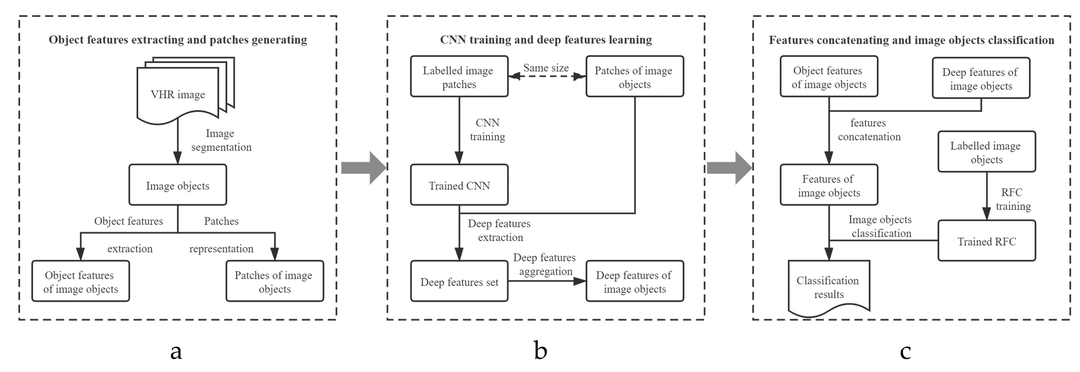
Figure 1. The framework of the proposed approach. (a) Object features extracting and patches generating, (b) CNN training and deep features learning, (c) features concatenating and image objects classification.
Remotesensing 12 03007 g001
Figure 2. Patches representation of an image object (the black line refers to an image object and the red lines represent patches).
Remotesensing 12 03007 g002
Figure 3. The structure of CB.
Remotesensing 12 03007 g003
Figure 4. A dense block (DB) composed of four convolutional blocks (CBs).
Remotesensing 12 03007 g004
Figure 5. The structure of the transition layer (TL).
Remotesensing 12 03007 g005
Figure 6. A DenseNet composed of three DBs.
Remotesensing 12 03007 g006
Figure 7. The flowchart of deep feature extraction for an image object: (a) the patch representation (patches are represented by red line while object boundaries are depicted in Cyan), (b) feature maps extracted by DenseNet (red color refers to high values and blue color represents low values), (c) feature maps after using compress function (mean operator), (d) the weights of patches, and (e) the final deep features of the image object.
Remotesensing 12 03007 g007
Figure 8. Study datasets. (a) Image of Beijing dataset, (b) reference map of Beijing dataset, (c) image of Zurich dataset, and (d) reference map of Zurich dataset.
Remotesensing 12 03007 g008
Figure 9. Land cover classification results of Beijing dataset (a) and Zurich dataset (b).
Remotesensing 12 03007 g009
Figure 10. The box plots of classification accuracies. (a) The box plot of overall accuracy of Beijing dataset; (b) the box plot of producer accuracy of Beijing dataset; (c) the box plot of overall accuracy of Zurich dataset; (d) the box plot of producer accuracy of Zurich dataset.
Remotesensing 12 03007 g010
Figure 11. O S e g , U S e g , and R M S values of Buildings (a), Vegetation (b), Roads (c), Water (d), Shadows (e) and Bare soils (f) at different scales.
Remotesensing 12 03007 g011
Figure 12. The variation of overall accuracies over segmentation scales (the horizontal axis refers to segmentation scale, the vertical axis refers to accuracies, and different curves represent different patch sizes).
Remotesensing 12 03007 g012
Figure 13. The variation of producer accuracies of Buildings (a), Vegetation (b), Roads (c), Water (d), Shadows (e) and Bare soils (f) over segmentation scales (the horizontal axis refers to segmentation scale, the vertical axis refers to accuracies, and different curves represent different patch sizes).
Remotesensing 12 03007 g013
Figure 14. Frequency distributions of O S e g and U S e g at scales of 50 and 210.
Remotesensing 12 03007 g014
Figure 15. (a) Oversegmentation and (b) undersegmentation (red lines represent geographic objects, and yellow lines represent image objects).
Remotesensing 12 03007 g015
Figure 16. The variation of overall accuracies over patch sizes (different curves represent different segmentation scales).
Remotesensing 12 03007 g016
Figure 17. The variation of producer accuracies of Buildings (a), Vegetation (b), Roads (c), Water (d), Shadows (e) and Bare soils (f) over patch sizes (the horizontal axis refers to patch size, the vertical axis refers to accuracies, while different curves represent different segmentation scales).
Remotesensing 12 03007 g017
Figure 18. Classification results of different features combinations. (a) Classification result with object features; (b) classification result with object features; (c) classification result with both object and deep features.
Remotesensing 12 03007 g018
Figure 19. Overall accuracies of different features combinations.
Remotesensing 12 03007 g019
Figure 20. Producer accuracies of Buildings (a), Vegetation (b), Roads (c), Water (d), Shadows (e) and Bare soils (f) with different feature combinations.
Remotesensing 12 03007 g020
Figure 21. Overall accuracies with or without deep feature aggregation.
Remotesensing 12 03007 g021
Figure 22. The methods to place patches of different approaches: (a) Fu et al.; (b) Zhao et al.; (c) Zhang et al.; and (d) ours. (black lines represent image objects and red lines represent patches).
Remotesensing 12 03007 g022
Figure 23. Classification results comparison of (a) Fu et al., (b) Zhao et al., (c) Zhang et al. and (d) our method on Beijing dataset.
Remotesensing 12 03007 g023
Figure 24. Classification results comparison of (a) Fu et al., (b) Zhao et al., (c) Zhang et al. and (d) our method on Zurich dataset.
Remotesensing 12 03007 g024
Table 1. Producer accuracy ( P A ) and user accuracy ( U A ) of each class of Beijing dataset (%).
BuildingsRoadsVegetationWaterShadowsBare Soils
P A 84.9994.7991.2597.7797.0596.07
U A 96.7194.8284.6683.7789.8981.92
Table 2. P A and U A of each class of Zurich dataset (%).
BuildingsRoadsRailwaysTreesGrassBare Soils
P A 99.0899.3199.8098.3498.8299.93
U A 99.4598.3798.0295.8799.5999.99
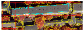
Table 3. Patch representations of image objects (yellow lines represent geographic objects and red lines represent patches) and the learned deep features (red represents high value and blue represent low value) with different patch sizes.
Patch SizePatch Representations of
Image Objects
Deep Features
(Only One Feature Map Is Shown)
16 Remotesensing 12 03007 i001 Remotesensing 12 03007 i002
24 Remotesensing 12 03007 i003 Remotesensing 12 03007 i004
32 Remotesensing 12 03007 i005 Remotesensing 12 03007 i006
40 Remotesensing 12 03007 i007 Remotesensing 12 03007 i008
48 Remotesensing 12 03007 i009 Remotesensing 12 03007 i010
56 Remotesensing 12 03007 i011 Remotesensing 12 03007 i012
64 Remotesensing 12 03007 i013 Remotesensing 12 03007 i014
Table 4. Comparison of classification accuracies on Beijing dataset (bold numbers represent the highest O A , the highest P A of each class, and the highest U A of each class).
Method O A (%)Class P A (%) U A (%)
Fu et al.83.34Buildings69.1095.43
Vegetation91.5794.18
Roads88.0665.29
Water94.8982.46
Shadows93.8685.10
Bare soils96.0959.25
Zhao et al.87.43Buildings76.6596.60
Vegetation93.2797.30
Roads90.6074.68
Water97.5380.21
Shadows96.0789.93
Bare soils94.6959.78
Zhang et al.88.78Buildings82.7596.01
Vegetation93.8394.21
Roads93.2976.46
Water94.5081.66
Shadows88.9590.97
Bare soils96.6274.53
This research91.21Buildings84.9996.71
Vegetation94.7994.82
Roads91.2584.66
Water97.7783.77
Shadows97.0589.89
Bare soils96.0781.92
Table 5. Comparison of classification accuracies on Zurich dataset (bold numbers represent the highest O A , the highest P A of each class, and the highest U A of each class).
Method O A (%)Class P A (%) U A (%)
Fu et al.95.40Buildings91.7998.16
Roads96.7986.22
Railways99.9798.97
Trees94.1987.37
Grass96.6398.44
Bare soils99.9499.51
Zhao et al.96.42Buildings95.8798.69
Roads97.2393.69
Railways98.0592.05
Trees95.4783.69
Grass95.7698.82
Bare soils99.8899.08
Zhang et al.98.53Buildings97.9099.45
Roads98.4397.68
Railways98.9397.49
Trees96.7695.30
Grass99.2198.60
Bare soils99.5699.91
This research99.05Buildings99.0899.45
Roads99.3198.37
Railways99.8098.02
Trees98.3495.87
Grass98.8299.59
Bare soils99.9399.99