Modelling of Impact Falling Ball Test Response on Solid and Engineered Wood Flooring of Two Eucalyptus Species

Abstract

In this study, dynamic hardness tests on solid and engineered wood flooring specimens of Eucalyptus globulus Labill. and Eucalyptus grandis W. Hill ex Maiden hardwoods were performed because nowadays, these fast-growing hardwoods are still scarcely employed for this use. Furthermore, another two examples of hardwood commonly applied on wood flooring, Quercus robur L. and Hymenaea courbaril L., were also tested. To compare their properties, a dynamic impact hardness test based on the impact of steel balls, with several diameters, and drop heights was developed. Accordingly, 120 solid wood flooring specimens and 120 engineering wood flooring specimens were producing with these four hardwood species. Dynamic impact tests were made with three steel balls of different diameters (30–40–50 mm), and they were carried out from five different drop heights (0.60–0.75–0.90–1.05–1.20 m). The impact of the steel ball drew the size of the footprint on the surface and this mark was measured with a digital caliper for both dimensions, diameter and depth, as footprint diameter (FD) and indentation depth (ID). Data from 3000 samples, corresponding to 120 different individual groups (4 species × 3 ball diameters × 5 drop height × 2 floor type) were analyzed. Results indicated that the variability of ID (CV between 19.25–25.61%) is much greater than the values achieved for FD (CV between 6.72–7.91%). Regarding the fast-growing hardwood species tested, E. globulus showed a similar behavior to traditional hardwood applied on wood flooring in Europe, Q. robur, and it could be a promising growth in the flooring industry. However, E. grandis showed the worst values compared to traditional hardwood in all test configurations.

1. Introduction

Nowadays, the use of wood flooring has increased in the building construction sector, due to industrial flooring quality improvement and cost reduction [1]. Besides, the manufacture of wood engineered flooring has significantly increased over wood solid flooring. This new product has allowed an increase in the stability of wood flooring by using multilayer gluing of wood derivative panels with a thin final layer of noble wood, producing a greater amount of floor volume with the same noble wood. Therefore, it has allowed a reduction in cost and an increase in competitiveness and quality with respect to solid floors [2,3,4]. However, despite wood flooring production increasing, only a few wood species are still used for flooring, mainly hardwood [5,6], and more recently, some softwood densified by some treatment [7,8]. Among the different species of wood available, the use of Eucalyptus stands out for its availability, sustainability and price [9]. These species, of Australian origin, have been widely cultivated in Spain, mainly Eucalyptus globulus Labill and to a lesser extent Eucalyptus grandis W. Hill ex Maiden, for the industrial extraction of cellulose, and more recently of structural wood [10]. Due to their high mechanical performance [11,12] and fast growth, they can be a profitable option for use in the wood flooring industry [13,14,15,16]. Consequently, this new use of this fast-growing species, widely used in reforestation for the pulp industry, could generate a new economic resource of higher added value.

To compare the performance of these lesser-used wood species for wood flooring, it is necessary to know several properties such as shrinkage stability, compression resistance, friction coefficient or hardness [17]. However, hardness is one of the most important features used to evaluate the surface properties of flooring materials [18,19,20,21]. There are a few standard methods for the determination of wood hardness, and most of them are just static test methods instead of dynamic test methods [22]. In Europe, the Brinell method is used to measure wood flooring hardness according to EN1534. In this test, a 10 mm diameter steel ball is indented, by a knowing static force, into wood specimen surface, and hardness is given by indentation’s depth (UNE-EN 1534:2020) [23]. In America, the Janka method is the most common, applied according to ASTM D 143:2000 [24]. In this test, an 11.284 mm diameter steel ball is indented into a known depth into the wood specimen surface, and the hardness is deduced by load applied (ASTM D 143:2000). Both methods have a good relationship between them, although each has disadvantages [25]. Meanwhile, in the Brinell method, the small diameter of the steel ball is used, drawing a small indentation over the wood surface, where it is difficult to accurately measure its depth [26,27]. Moreover, the recovery of the elastic portion of the notch can significantly affect the precision of the measurements [28,29,30]. On the other hand, in the Janka method, the application of an excessive load to indent the half ball diameter sometimes generates ruptures in the wood fibers around the test point, distorting the results obtained [31].

However, dynamic hardness tests (impacts) on the surface wood are more interesting for industrial flooring than static load tests because they can better simulate wood flooring performance in service [18,32]. Some researchers have tested a wide variety of masses and drop heights of steel balls, and the selected parameter combination provides user-friendly equipment with acceptable sensitivity to hardness variations [33]. However, beyond these previous investigations, the assessment of dynamic standards, flooring quality and wood characterization for floorings are still scarce.

The aims of this paper were: 1—to evaluate the behavior of new species of fast-growing hardwood, blue gum (Eucalyptus globulus) and rose gum (Eucalyptus grandis), without current use in the wood flooring industry, through of dynamic hardness tests carried out with steel balls of different diameters and from different drop height, over solid and engineered wood flooring samples; 2—to compare the results obtained, the same tests were carried out over two traditional hardwood species successfully used to wood flooring as oak (Quercus robur L.) and jatoba (Hymenaea courbaril L.); 3—to select a model that predicts dynamic hardness test response on solid and engineered wood flooring and to present a suitable robust analysis methodology in the trends modelling and prediction. 4—to evaluate if this new use of these fast-growing species can be possible.

2. Materials and Methods

2.1. Wood Species

In the present experimental programme, four different hardwood species were used. Two of them are commonly applied on wood flooring as Quercus robur L. and Hymenaea courbaril L., and other two fast-growing hardwood without current wood flooring application as Eucalyptus globulus Labill and Eucalyptus grandis W. Hill ex Maiden. The batch of oak wood was provided from a sawmill from Milicz (Poland), and the jatoba wood was bought from a Spanish wood importer and it was harvested from Brazil. Both Eucalyptus species were provided from existing plantations in Arzúa and Curtis (Galicia, Spain). Each wood species comes from the same sawmill and it was bought in a single batch, aiming statistically reduce the variability on wood physical properties due to different environmental conditions during growing. All timber was selected without visual defects, and, once they arrived at the laboratory, they were maintained under controlled conditions of a temperature of 20 °C (±2 °C), and an air relative humidity of 65% (±5%) according to EN 408:2011 [34]. After 3 months, timber pieces were considered stabilized, and density of wood of different species was measured in accordance with standard EN 13183:2002 [35] (

Table 1. Wood flooring types, species and properties.

	Solid Wood Flooring			Engineered Wood Flooring
Species	Nº of Pieces/Impacts	Nominal Size (l × w × t *) (mm)	Density (kg·m−3)	Nº of Pieces/Impacts	Nominal Size (l × w × t) * (mm)
Oak (Q. robur L.)	30/150	300 × 70 × 25	686.1 (9.1 **)	30/450	1000 × 200 × 14
Jatoba (H. courbaril L)	30/450	300 × 70 × 25	954.6 (10.4 **)	30/450	1000 × 200 × 14
Blue gum (E. globulus Labill)	30/150	300 × 75 × 16	854.8 (11.3 **)	30/450	1000 × 200 × 14
Rose gum (E. grandis W. Hill)	30/450	300 × 75 × 16	488.3 (9.8 **)	30/450	1000 × 200 × 14

* l: length; w: width; t: thickness; ** Coefficient of variation (CV) measured in %.

).

2.2. Wood Flooring Specimens

Two wood flooring types, solid wood and engineered wood, were tested. Both types were made specifically for this research. The engineered wood floorings were made up of three layers. A noble top layer of 3 mm thickness of manufacture with one of the hardwood species was analyzed. In the middle, a support layer of 9 mm thickness of waterproof high-density fiberboard (density of 850 kg·m⁻³). There was an additional bottom veneer layer of 2 mm thickness of Pinus radiata D. Don (density of 500 kg·m⁻³). All wood layers were glued with urea–formaldehyde resin type E1. The main specimen characteristics are shown in Table 1.

2.3. Impact Test

To evaluate the wood dynamic hardness, an experimental campaign was planned on solid and engineered wood flooring specimens by impact test. According to standard ASTM D1037-99 [36], wood hardness could define the measuring of the diameter of the impact footprint of a 536 g and 50 mm diameter steel ball in its free fall from a determined height. This standard allows for the testing of the wood hardness without the need for sophisticated equipment, just a steel ball. However, it is common in some wood species that this test produces excessive impact energy causing a perimeter breakage of wood fibers and hindering the precise measurement of a footprint. For that reason, this experimental work included the testing of wood hardness with three steel balls of different sizes (diameters 30–40–50 mm), and testing each one from 5 different reference heights (0.60–0.75–0.90–1.05–1.20 m). Steel ball characteristics and impact energy are shown in

Table 2. Steel ball characteristics and impact energy.

Nominal Diameter (mm)	Weight (g)	Impact Energy (J) *
		h = 0.60 m	h = 0.75 m	h = 0.90 m	h = 1.05 m	h = 1.20 m
50	508.8	2.99	3.74	4.49	5.24	5.99
40	260.5	1.53	1.92	2.30	2.68	3.07
30	109.9	0.65	0.81	0.97	1.13	1.29

* Impact energy: Ep = m ∗ g ∗ h.

.

The impact test allows us to obtain knowledge on the behavior of the solid and engineered wood flooring through deformation produced by the steel ball, allowing us to compare the behavior of new fast-growing hardwood species, such as Eucalyptus globulus and Eucalyptus grandis, with more common and well-known hardwood species such as Quercus robur and Hymenaea courbaril. The sample of each group (4 hardwood species and 2 wood flooring types; solid and engineered) consisted of 30 pieces from each group, with dimensions (l × w × t) of 300 × 70/75 × 19/25 mm for solid wood specimens, and 1000 × 200 × 14 mm for engineered ones. These test specimen dimensions are chosen because they are the most common on wood flooring. On each specimen, 5 hits were made at least 50 mm apart, and a total impact test of 3000 hits was tested as indicated in Table 1. The steel ball impact, for flooring types and wood species, was measured in two ways in each test specimen: footprint diameter (FD), and indentation depth (ID).

The impact test specimen’s main dimensions and impacts test localization are shown in Figure 1.

To carry out each impact test, flooring specimens were placed on a completely rigid surface and anchored to it by clamps placed on the perimeter, avoiding any influence of the support on the deformation behaviour. Later, each ball was dropped from each of the reference heights on one of the test specimen, using an auxiliary metallic instrument to guarantee the test conditions (precise height reference, and initial velocity V₀ = 0 m/s), Figure 2.

To improve the impact reading, a sheet of carbon paper is placed on the test specimen surface, to draw the size of the footprint on it. The deformation of the surface layer was measured for ID with a digital caliper (error ± 0.01 mm), and for FD with a digital micrometre (error 0.001 mm). Due to the footprint, an appreciably elliptical deformation is caused owing to the different compressive strengths in the parallel direction, and perpendicular to the fibers, the footprint diameter was calculated as the average between the largest (D1-fiber direction) and the minor (D2-transverse to the fiber). The steel ball impact test was assessed through the diameter of the footprint and the possible breakage of the wood fibre, which must not exceed 50% of the perimeter, and the average of the impact footprint diameters must be less than 12.5 mm.

2.4. Statistical Analysis

All the statistical analyses were performed using R software (v. 3.6.1:2019). The diameter steel ball and drop height were selected to establish statistical design according to ASTM D1037-99 standard [36] and AITIM recommendations [37]. For each group (species × ball diameters × drop height × floor type), the number of essays was established through initial and traditional variability analysis which was realized with 800 tests. In accordance with this, the number of repetitions (n) obtained with a confidence level of 95% was 26 tests. However, to ensure and to obtain the appropriate design performance, 30 tests by group were realized in this work. Data from 3000 samples, corresponding to 120 different individual groups (4 species × 3 ball diameters × 5 drop height × 2 floor type), were analyzed. Firstly, the assumptions of independence, normality and homoscedasticity were verified for the studied variables: footprint diameter (FD) and indentation depth (ID) in each of the 120 sample groups. The normality of the data was checked for all populations using the Kolmogorov–Smirnov normality test with Lilliefors correction, the Shapiro–Wilk test and the Q–Q normal probability plot. The requirement of homoscedasticity was contrasted by the Bartlett test, being defaulted on numerous occasions, so the usual comparative analysis that provides linear statistics, ANOVA, cannot be used. To solve this impediment, robust comparison methods were used: Welch’s heteroscedastic F test with trimmed means and Winsorized variances a robust procedure that tests the equality of means by substituting trimmed means and Winsorized variances for the usual means and variances [38,39], along with bootstrapping and robust homogenous groups.

2.5. Modelling of Impact Falling Ball Test

2.5.1. Model Development and Selection

First, generalized linear regression with all 4 predictive variables (V1: ball diameter—numerical variable, V2: species—categorical variable, V3: floor type—categorical variable, V4: drop height—numerical variable) was applied. After, model selection in the framework of generalized linear models was performed. Considering our data structure, the type of variables that compose it and the general presence of heteroscedasticity among its groups, it was decided to model the behavior of the impact, measured like footprint diameter (FD) and indentation deep (ID), using Generalized Linear Model (GLM). In this sense, Nelder and Wedderburn [40] proposed family generalized linear models that unified some existing models in a single class. The basic idea of these models consists of opening the range of options for the response variable distribution, permitting that the same one belongs to the exponential family of distributions, which also brings a profit in the question of model interpretation. In accordance with these authors and with Dobson [41], the function of linking the data plays the role to relate the average to the linear predictor. However, currently, the GLMs have extended to multivariate exponential families (such as the multinomial distribution), to certain non-exponential families (such as the two-parameter negative-binomial distribution), and to some situations in which the distribution of Yi is not specified completely.

To formulate a GLM, a link function, which relates the linear predictors to the predicted mean of response, is required, along with a function defining the error probability distribution around the mean. Examples of distributions that belong to the exponential family are Normal, Binomial, Poisson, Gamma, and so on. Essentially, the choice of link function is rather subjective [42] and it is necessary to check by means of plots and tests the adequacy of the error response.

(A) Residual Analysis

The main purpose of residual analysis in a GLM is to identify model mix-specification or outliers. Since a well-fitting model is a prerequisite for reliable inferences, it is, therefore, necessary to inspect the quality of fit provided by the regression model, after fitting the model to a set of data.

(B) Residual Deviance

The lack of fit in GLM regression is measured by deviance, which provides a measure of the discrepancy between the model and the data. A large value of deviance indicates a poor fit, while a small value of deviance indicates a good fit [43].

(C) Akaike Information Criteria (AIC) and Bayesian Information Criteria (BIC)

In many instances, a key step in the analysis is to ask which of several alternative models best explains the data [44]. P-values are an insufficient measure of the appropriateness of alternative models [44,45], and a much better alternative is to use some form of information criteria, such as the Akaike Information Criteria (AIC) or the Bayesian Information Criteria (BIC). These are based on the principle of parsimony, helping to identify the model that accounts for the most variation with the fewest variables. AIC tends to select models with too many parameters when sample sizes are large, whereas BIC may be too conservative, yielding overly simplistic models because of the heavy penalty on the addition of additional parameters [46].

For competing generalized linear regression models, the best model can be determined by taking into account the number of parameters, using the AIC. This measure describes the trade-off between bias and variance in model construction, or between accuracy and complexity of the model [42,44,47]. It is a measure of fit that penalizes the number of parameters. When models differ in terms of their link functions or predictors, comparing AIC statistic is straightforward. However, the same data should be fitted by models that are being compared. Smaller values of AIC indicate better fit, and thus the AIC can be used to compare models, whether nested or not [43]. The BIC criterion [48] can be derived using Bayesian methods as discussed by Chen and Chen [49]. The model with the smallest BIC corresponds to the model with maximum posterior probability. The difference between these criteria is in the penalty. When n > 7, the BIC penalty is always larger than for the AIC and consequently the BIC will never select models with more parameters than the AIC. In practice, the BIC often selects more parsimonious models than the AIC.

Different Gaussian and Gamma models with different link functions were tested.

2.5.2. Model Diagnostic

To validate the selected model, diagnostic graphics were used. Linearity, where there was no trend in the residuals, was checked and assumed for both FD and ID models.

2.5.3. Prediction and Validation

Validation was carried out checking the model prediction ability with external bibliographic data [50,51,52].

3. Results and Discussion

The analysis of the steel ball impact measured through its footprint diameter (FD), and its indentation depth (ID) are shown and compared, for flooring types and wood species, below.

3.1. Footprint Diameter (FD)

Different groups corresponding to the different combinations between wood flooring type, wood species, drop height and steel ball diameter (Φ), were statistically analyzed. Main footprint diameter (FD) values (in cm) and their coefficients of variation (CV) for all these combinations are shown in

Table 3. Footprint diameter (FD). Main descriptive statistics.

	Solid Wood Flooring (SWF)			Engineered Wood Flooring (EWF)
Height	Φ 50 mm	Φ 40 mm	Φ 30 mm	Φ 50 mm	Φ 40 mm	Φ 30 mm
	E. globulus
1.20 m	13.74	11.05	8.59	12.78	10.05	7.72
	(9.57) 0.1827 *	(12.45) 0.1274 *	(6.89) 0.1525 *	(8.57) 0.0681 *	(10.66) 0.2018 *	(14.23) 0.6422 *
1.05 m	14.38	11.14	8.24	12.48	9.79	7.48
	(2.72) 0.8420 *	(5.75) 0.7633 *	(3.91) 0.4223 *	(9.14) 0.4584 *	(10.46) 0.1361 *	(6.46) 0.0520 *
0.90 m	13.77	10.73	7.52	12.05	9.67	7.13
	(5.11) 0.0836 *	(7.01) 0.7221 *	(7.42) 0.1009 *	(8.17) 0.9492 *	(10.38) 0.4191 *	(9.77) 0.5336 *
0.75 m	12.69	9.82	7.19	11.56	8.98	7.00
	(7.14) 0.0495 *	(8.31) 0.2154 *	(8.40) 0.9949 *	(10.47) 0.2484 *	(7.80) 0.4405 *	(10.96) 0.9294 *
0.60 m	11.94	9.66	6.99	11.03	8.52	6.39
	(9.06) 0.3414 *	(5.65) 0.2543 *	(3.62) 0.8008 *	(11.09) 0.2563 *	(10.95) 0.1576 *	(12.60) 0.4577 *
E. grandis
1.20 m	18.27	13.65	10.15	15.17	11.39	8.63
	(6.62) 0.3259 *	(4.35) 0.6817 *	(9.21) 0.3950 *	(6.62) 0.6440 *	(4.33) 0.4621 *	(12.57) 0.3904 *
1.05 m	17.46	12.56	9.76	14.56	10.60	7.70
	(8.17) 0.3886 *	(7.41) 0.3204 *	(7.23) 0.1444 *	(8.17) 0.0525 *	(4.16) 0.1673 *	(12.56) 0.2805 *
0.90 m	16.64	12.26	9.89	13.88	10.05	7.84
	(7.97) 0.1838 *	(9.88) 0.4595 *	(6.74) 0.2404 *	(7.97) 0.1599 *	(7.46) 0.5368 *	(7.31) 0.9575 *
0.75 m	16.69	11.51	8.93	12.92	9.72	7.26
	(5.25) 0.9129 *	(8.55) 0.6479 *	(6.26) 0.5137 *	(5.25) 0.5169 *	(8.21) 0.4977 *	(5.66) 0.3510 *
0.60 m	14.65	11.18	8.28	12.66	9.29	6.93
	(8.42) 0.5391 *	(6.47) 0.9554 *	(5.76) 0.3923 *	(6.06) 0.1106 *	(6.82) 0.9821 *	(8.27) 0.3850 *
H. courbaril
1.20 m	10.80	8.94	7.69	10.18	8.12	6.40
	(5.90) 0.5247 *	(4.94) 0.7940 *	(3.22) 0.5049 *	(5.27) 0.5041 *	(6.11) 0.2670 *	(6.62) 0.4060 *
1.05 m	10.33	8.01	7.20	9.28	7.68	6.34
	(4.18) 0.5157 *	(8.84) 0.2151 *	(4.50) 0.2345 *	(8.57) 0.5574 *	(6.44) 0.3707 *	(4.39) 0.4979 *
0.90 m	9.82	8.05	6.72	9.06	7.50	5.83
	(4.00) 0.4358 *	(4.80) 0.1256 *	(3.98) 0.6787 *	(5.53) 0.9318 *	(3.53) 0.6316 *	(8.09) 0.4809 *
0.75 m	9.57	7.71	6.57	8.41	6.74	5.78
	(4.85) 0.3640 *	(4.09) 0.5652 *	(6.51) 0.1398 *	(8.79) 0.2842 *	(3.72) 0.9730 *	(4.12) 0.2709 *
0.60 m	9.06	7.26	6.07	7.85	6.55	5.77
	(5.34) 0.3627 *	(6.61) 0.5163 *	(4.56) 0.7879 *	(7.71) 0.4798 *	(4.56) 0.6901 *	(8.43) 0.4758 *
Q. robur
1.20 m	14.10	11.45	8.66	12.89	10.38	7.83
	(5.93) 0.1593 *	(8.05) 0.1486 *	(8.55) 0.4531 *	(9.68) 0.3466 *	(11.12) 0.4838 *	(9.32) 0.6585 *
1.05 m	13.32	10.77	8.46	13.14	10.31	7.61
	(8.35) 0.2208 *	(7.12) 0.5532 *	(9.25) 0.9602 *	(3.88) 0.1747 *	(7.00) 0.8050 *	(8.69) 0.9895 *
0.90 m	13.48	10.80	8.26	12.24	9.55	7.16
	(3.05) 0.4346 *	(8.64) 0.9505 *	(7.36) 0.2211 *	(5.99) 0.7939 *	(10.02) 0.9541 *	(8.39) 0.2331 *
0.75 m	13.06	10.71	8.13	11.95	9.18	7.09
	(9.71) 0.7198 *	(8.44) 0.1935 *	(9.69) 0.6854 *	(7.82) 0.7497 *	(9.54) 0.8067 *	(7.90) 0.3736 *
0.60 m	11.71	9.88	7.44	11.56	8.65	6.50
	(6.14) 0.7400 *	(9.02) 0.9974 *	(6.45) 0.7442 *	(6.73) 0.2864 *	(9.16) 0.4378 *	(7.43) 0.8355 *

Mean values in mm, appear in bold font; () Coefficients of variation, CV (%) are shown between parentheses; * Shapiro–Wilk normality test—p-value.

. The p-value of the Shapiro–Wilk normality test was >0.05 in all the groups, which allows us to assume the normality of all of them.

As expected, the footprint diameter (FD) values showed a clear tendency to increase when the drop height and ball diameter increased too. This behavior can be seen graphically in Figure 3.

Regarding the behaviour (Table 3 and Figure 3) of solid wood flooring (SWF) versus engineered wood flooring (EWF), the overall values of the footprint diameter (FD) in SWF, for the same species conditions, ball diameter and drop height, were significantly higher in all cases. The range of FD values for SWF was between 5.47 and 21.40 mm, while for EWF, it was between 4.76 and 16.84 mm. For the values by species, keeping the rest of the variables constant, the highest values were presented for E. grandis, with main EWF values between 6.93 and 15.17 mm, showing worse behaviour than the rest of the studied species. However, the values obtained by E. globulus, with average EWF values between 6.39 and 12.78 mm, were similar to traditional wood species analysis such as Q. robur, with values between 6.50 and 12.89 mm, or H. courbaril, with values between 6.93 and 10.18 mm.

The mean global variability of the variable of FD in SWF, expressed as CV, was 6.724%, lower than EWF with a variability of 7.912%. The statistical analysis carried out showed a statistically significant difference between these mean values.

3.1.1. Pairwise Comparison for FD between Wood Flooring Types (SWF and EWF)

In accordance with the Bartlett test, in most cases, the homoscedastic requirement for dates was not achieved. For this reason, an alternative method to ANOVA, Welch’s heteroscedastic F test with trimmed means and Winsorized variances [39], was applied (

Table 4. Pairwise comparison footprint diameter (FD) of solid wood flooring (SWF) vs footprint diameter (FD) of engineered wood flooring (EWF) for the same drop height and same ball.

	Φ 50 mm					Φ 40 mm					Φ 30 mm
Height (m)	0.60	0.75	0.90	1.05	1.20	0.60	0.75	0.90	1.05	1.20	0.60	0.75	0.90	1.05	1.20
Q. robur	=	x	x	=	x	x	x	x	=	x	x	x	x	x	x
E. globulus	x	x	x	x	=	x	x	x	x	x	x	=	=	x	x
E. grandis	x	x	x	x	x	x	x	x	x	x	x	x	x	x	x
H. courbaril	x	x	x	x	x	x	x	x	x	x	x	x	x	x	x

x: Difference is statistically significant. Welch’s Heteroscedastic F Test (alpha = 0.05) p-value < 0.05. =: Difference is not statistically significant, p-value > 0.05.

).

In Table 4 stand out SWF-EWF pairs that, for the same test conditions (same drop height and same ball diameter) have presented statistically significant differences.

3.1.2. Pairwise Comparison for FD between Wood Species (to Each Wood Flooring Types)

Post-hoc pairwise comparisons for FD between wood species per type wood flooring, drop height and Φ ball are shown in

Table 5. FD Pairwise comparison for species per wood flooring types and drop height x Φ ball.

Solid Wood Flooring (SWF)

Φ 50 mm

Φ 40 mm

Φ 30 mm

Height (m)

0.60

0.75

0.90

1.05

1.20

0.60

0.75

0.90

1.05

1.20

0.60

0.75

0.90

1.05

1.20

Q. robur

b

b

b

c

b

b

a b

b

b

b

c

c

c

b

b

E. globulus

b

b

b

b

b

b

b

b

b

b

b

b

b

b

b

E. grandis

a

a

a

a

a

a

a

a

a

a

a

a

a

a

a

H. courbaril

c

c

c

d

c

c

c

c

c

c

d

d

d

c

c

Engineered Wood Flooring (EWF)

Φ 50 mm

Φ 40 mm

Φ 30 mm

Height (m)

0.60

0.75

0.90

1.05

1.20

0.60

0.75

0.90

1.05

1.20

0.60

0.75

0.90

1.05

1.20

Q. robur

c

b

b

c

b

b

b

a

a b

b

b

a b

b

a b

b

E. globulus

b

b

b

b

b

b

b

a

b

b

b

b

b

b

b

E. grandis

a

a

a

a

a

a

a

a

a

a

a

a

a

a

a

H. courbaril

d

c

c

d

c

c

c

b

c

c

c

c

c

c

c

Different letters on each column (a, b, c and d) indicate significant differences (p value < 0.05).

.

In accordance with Table 5, post-hoc pairwise comparisons showed that there was a significant difference between H. courbaril with the rest of the wood species in all possible test conditions (drop height and Φ ball). Moreover, lower FD values were always shown. On the other hand, E. grandis is the species that shows the highest FD values in the vast majority of test conditions. Finally, the similar behavior of the Q. robur and E. globulus species is worth noting, which in most cases does not show significant differences.

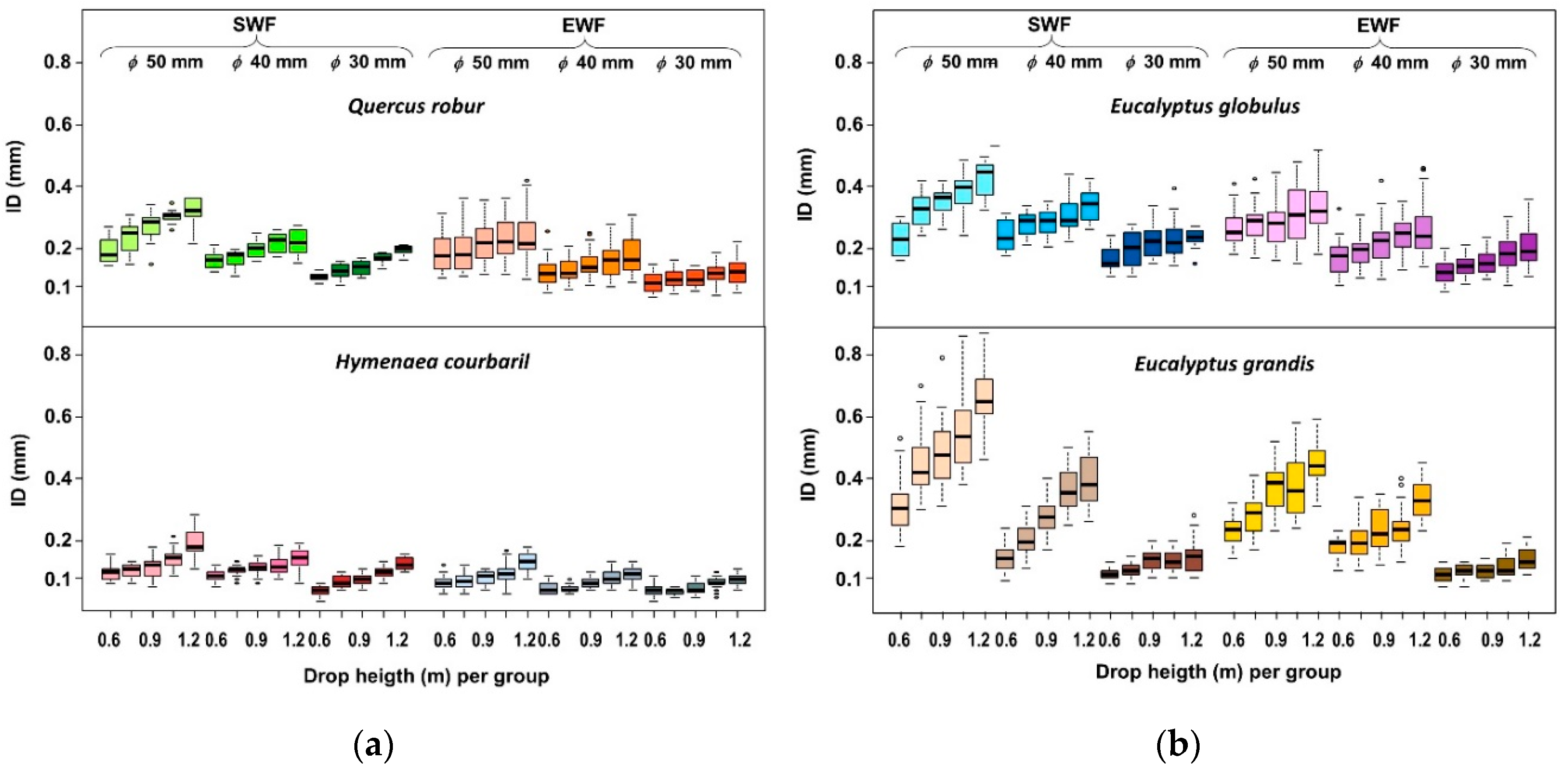
3.2. Indentation Depth (ID)

In this second analysis, measuring indentation depth (ID) of steel ball impact, different groups were analyzed, corresponding to the different combinations between flooring type, wood species, drop height and steel ball diameter. Main ID values (in mm) and their CV (%) with all the test combination results are shown in

Table 6. Indentation depth (ID). Main descriptive statistics.

	Solid Wood Flooring			Engineered Wood Flooring
Height	Φ 50 mm	Φ 40 mm	Φ 30 mm	Φ 50 mm	Φ 40 mm	Φ 30 mm
	E. globulus
1.20 m	0.252	0.200	0.138	0.331	0.263	0.206
	(14.03) 0.2978 *	(16.67) 0.5647 *	(25.92) 0.2509 *	(27.65) 0.06104 *	(33.64) 0.0080 *	(25.92) 0.6793 *
1.05 m	0.223	0.180	0.139	0.313	0.247	0.184
	(19.00) 0.6451 *	(19.91) 0.2026 *	(29.68) 0.3278 *	(28.70) 0.4577 *	(23.16) 0.7085 *	(29.68) 0.7952 *
0.90 m	0.208	0.169	0.134	0.275	0.221	0.155
	(14.40) 0.5809 *	(15.76) 0.9935 *	(23.32) 0.7721 *	(23.85) 0.7111 *	(28.77) 0.5392 *	(23.32) 0.1498 *
0.75 m	0.194	0.167	0.118	0.278	0.194	0.143
	(18.63) 0.6777 *	(24.54) 0.7542 *	(21.34) 0.5954 *	(20.31) 0.4314 *	(24.70) 0.2987 *	(21.34) 0.9729 *
0.60 m	0.137	0.143	0.100	0.262	0.169	0.122
	(23.86) 0.2260 *	(20.56) 0.3949 *	(28.64) 0.3010 *	(19.24) 0.0603 *	(27.77) 0.2489 *	(28.64) 0.6362 *
E. grandis
1.20 m	0.674	0.393	0.144	0.445	0.331	0.137
	(13.66) 0.3177 *	(21.02) 0.3252 *	(33.68) 0.0223	(15.99) 0.6821 *	(17.12) 0.8061 *	(24.41) 0.0705 *
1.05 m	0.558	0.369	0.135	0.370	0.243	0.116
	(22.32) 0.1250 *	(19.56) 0.1708 *	(25.33) 0.3171 *	(26.88) 0.0940 *	(26.28) 0.2100 *	(29.47) 0.0153
0.90 m	0.481	0.274	0.138	0.370	0.233	0.100
	(23.10) 0.4694 *	(22.00) 0.4704 *	(22.95) 0.6653 *	(20.83) 0.5546 *	(28.02) 0.4308 *	(21.18) 0.0153
0.75 m	0.441	0.206	0.103	0.282	0.200	0.101
	(21.50) 0.1049 *	(24.20) 0.7412 *	(22.25) 0.5623 *	(22.30) 0.7861 *	(30.46) 0.0499 *	(19.17) 0.0412
0.60 m	0.324	0.143	0.091	0.230	0.180	0.091
	(28.78) 0.0306	(29.56) 0.4790 *	(16.67) 0.1248 *	(18.73) 0.7997 *	(16.70) 0.1770 *	(27.73) 0.0478
H. courbaril
1.20 m	0.188	0.145	0.136	0.140	0.107	0.090
	(19.92) 0.1972 *	(14.96) 0.0229	(20.87) 0.0205	(22.48) 0.2284 *	(21.92) 0.2459 *	(25.12) 0.0785 *
1.05 m	0.148	0.127	0.113	0.106	0.095	0.082
	(16.90) 0.8213 *	(11.87) 0.4255 *	(19.42) 0.0416 *	(24.92) 0.0685 *	(15.05) 0.4364 *	(17.05) 0.0812 *
0.90 m	0.124	0.121	0.090	0.094	0.083	0.066
	(22.96) 0.5623 *	(15.68) 0.1132 *	(17.80) 0.1366 *	(15.70) 0.0257 *	(15.86) 0.0877 *	(26.90) 0.0072 *
0.75 m	0.116	0.114	0.084	0.086	0.065	0.055
	(14.83) 0.0794 *	(19.45) 0.0918 *	(11.16) 0.0186 *	(26.85) 0.1989 *	(20.19) 0.0046 *	(19.58) 0.0028 *
0.60 m	0.110	0.097	0.060	0.082	0.065	0.063
	(19.10) 0.0795 *	(20.32) 0.1033 *	(12.04) 0.0102 *	(17.87) 0.2330 *	(19.41) 0.0011 *	(14.09) 0.2429 *
Q. robur
1.20 m	0.323	0.226	0.198	0.244	0.177	0.132
	(15.66) 0.0894 *	(18.59) 0.7587 *	(8.00) 0.1759 *	(34.37) 0.0777 *	(34.47) 0.1052 *	(0.323) 0.0809 *
1.05 m	0.311	0.223	0.170	0.231	0.159	0.122
	(7.90) 0.9437 *	(14.46) 0.4078 *	(11.25) 0.1149 *	(29.99) 0.6467 *	(34.85) 0.1068 *	(0.311) 0.7232 *
0.90 m	0.276	0.204	0.138	0.227	0.155	0.101
	(20.42) 0.1422 *	(16.00) 0.6060 *	(16.49) 0.3931 *	(28.25) 0.3705 *	(28.40) 0.0531 *	(0.276) 0.0674 *
0.75 m	0.238	0.169	0.127	0.195	0.129	0.101
	(22.79) 0.6361 *	(16.55) 0.1654 *	(22.13) 0.5434 *	(37.66) 0.0081 *	(29.11) 0.5753 *	(0.238) 0.4062 *
0.60 m	0.192	0.164	0.107	0.187	0.125	0.091
	(22.50) 0.2240 *	(16.31) 0.9113 *	(12.13) 0.8374 *	(32.40) 0.0954 *	(38.64) 0.4118 *	(0.192) 0.0832 *

Mean values in mm, appear in bold font; (): Coefficient of variation—CV (%) is shown between parentheses; * Shapiro–Wilk normality test—p-value.

. Furthermore, all the data were subjected to statistical analysis. In the case of ID, not all groups have a p-value > 0.05 in the Shapiro–Wilk normality test, and the requirement of normality cannot be assumed in many groups, especially in the Hymenaea courbaril and Eucalyptus grandis species.

As with footprint diameter (FD) values, the indentation depth (ID) values had a clear tendency to increase their values when the drop height and the diameter of the ball increased too. This behavior can be seen graphically in Figure 4.

Regarding the behavior of solid wood flooring (SWF) versus engineered one (EWF) (Table 6 and Figure 4), the overall values of the indentation depth (ID) in SWF, for the same species conditions, ball diameter and drop height, were significantly higher in all cases. The range of ID values for SWF was between 0.030 and 0.870 mm, while for engineered wood flooring (EWF), groups were between 0.030 and 0.590 mm. For the values by species, keeping the rest of the variables constant, the highest values were presented for E. grandis, with main values between 0.091 and 0.445 mm, showing worse behaviour than the rest of the studied species. However, the values obtained by E. globulus, with average EWF values between 0.122 and 0.331 mm, are similar to traditional wood species analysis as Q. robur, with values between 0.091 and 0.244 mm, or H. courbaril, with values between 0.063 and 0.140 mm.

The mean global variability of the variable of ID, expressed as CV, was 19.25% and 25.61% for SWF and EWF, respectively. The statistical analysis carried out showed a statistically significant difference between these mean values. Furthermore, values achieved indicate that the variability of ID is much greater than that values achieved for FD.

3.2.1. Behaviour Comparison of ID Values: SWF vs. EWF

In accordance with the Bartlett test, in most cases for two types of wood flooring specimens (SWF and EWF), the homoscedastic requirement for dates was not achieved. Pairwise comparison ID SWF vs. ID EWF is displayed in

Table 7. Pairwise comparison indentation depth (ID) of solid wood flooring (SWF) vs indentation depth (ID) of engineered wood flooring (EWF) for the same drop height and same ball.

	Φ 50 mm					Φ 40 mm					Φ 30 mm
Height (m)	0.60	0.75	0.90	1.05	1.20	0.60	0.75	0.90	1.05	1.20	0.60	0.75	0.90	1.05	1.20
Q. robur	=	=	∗	∗	∗	∗	∗	∗	∗	∗	=	∗	∗	∗	∗
E. globulus	∗	∗	∗	∗	∗	∗	=	∗	∗	∗	=	=	=	=	∗
E. grandis	∗	∗	∗	∗	∗	∗	=	∗	∗	∗	=	=	∗	∗	=
H. courbaril	∗	∗	∗	∗	∗	∗	∗	∗	∗	∗	=	∗	∗	∗	∗

∗: Difference is statistically significant. Welch’s Heteroscedastic F Test (alpha = 0.05) p-value < 0.05; =: Difference is not statistically significant, p-value > 0.05.

.

In Table 7, stand-out SWF–EWF pairs, for the same test conditions (same drop height and same ball diameter), presented statistically significant differences.

3.2.2. Pairwise Comparison for ID between Wood Species

Post-hoc pairwise comparisons for ID between species per wood flooring type, drop height and Φ ball are shown in

Table 8. Indentation depth (ID) pairwise comparison for specie per type flooring and height × ball.

Solid Wood Flooring (SWF)

Φ 50 mm

Φ 40 mm

Φ 30 mm

Height (m)

0.60

0.75

0.90

1.05

1.20

0.60

0.75

0.90

1.05

1.20

0.60

0.75

0.90

1.05

1.20

Q. robur

c

b

b

b

b

a

b

c

b

b

b

a

a

b

b

E. globulus

b

b

c

c

c

a

b

b

c

b

ab

a

a

abc

a

E. grandis

a

a

a

a

a

a

a

a

a

a

a

a

a

a

a

H. courbaril

d

c

d

d

d

b

d

d

d

c

c

b

b

c

c

Engineered Wood Flooring (EWF)

Φ 50 mm

Φ 40 mm

Φ 30 mm

Height (m)

0.60

0.75

0.90

1.05

1.20

0.60

0.75

0.90

1.05

1.20

0.60

0.75

0.90

1.05

1.20

Q. robur

b

b

b

b

b

b

b

b

b

b

a

a

a

a

a

E. globulus

c

b

c

c

c

a

a

a

a

c

b

b

b

b

b

E. grandis

a

a

a

a

a

a

a

a

a

a

a

a

a

a

a

H. courbaril

d

c

d

d

d

c

c

c

c

d

c

c

c

c

c

Different letters on each column (a, b, c, and d) indicate significant differences (p-value < 0.05).

.

Post-hoc pairwise comparisons showed an analogy behavior of ID with FD, and that there was a significant difference between H. courbaril with the rest of the wood species in all possible test conditions (drop height and Φ ball), showing, in all cases, the lowest ID values. On the other hand, E. grandis is the species that showed the highest ID values in the vast majority of test conditions. Finally, as with FD analysis, similar behavior is observed between Q. robur and E. globulus species, especially in the EWF.

3.3. Model Selection

The summary of the select models for both FD and ID with the main statistics is shown in

Table 9. Summary of the best-fit Generalized Linear Model (GLM) for footprint diameter (FD) and indentation depth (ID).

Model		Family (Link)	AIC (Akaike Information Criteria)		BIC (Bayesian Information Criteria)		Log— Likelihood		D2 MacFadden		Pseudo R2 CoxSnell
			FD	DI	FD	DI	FD	DI	FD	DI	FD	DI
Y* = V1 + V2 + V3 + V4	1	Gaussian (identity)	−4934	−7000	−4880	−6952	2475.9	2475.9	86.35	63.88	0.86	0.64
	2	Gaussian (log)	−6077	−8295	−6023	−8247	3047.6	4155.7	90.68	76,55	0.91	0.77
	3	Gaussian (inverse)	−6278	−8377	−6224	−8329	3147.8	4196.6	91.28	77.18	0.91	0.77
Y* = V1 ∗ V2 ∗ V3 ∗ V4	4	Gaussian (identity)	−6687	−9130	−6392	−8932	3392.4	4597.9	92.59	82.53	0.93	0.83
	5	Gaussian (log)	−6681	−9046	−6387	−8848	3389.6	4556.0	92.58	82.04	0.93	0.82
	6	Gaussian (inverse)	−6673	−8799	−6379	−8601	3385.6	4432.3	92.56	80.50	0.93	0.80
Y* = V1 + V2 + V3 + V4	7	Gamma (inverse)	−6561	−9699	−6590	−9633	3330.8	4848.4	91.12	73.11	0.91	0.72
	8	Gamma (log)	−6402	−9654	−6348	−9606	3209.9	4835.0	90.38	73.97	0.90	0.74
Y* = V1 ∗ V2 ∗ V3 ∗ V4	9	Gamma (inverse)	−7080	−10,390	−6786	−10,192	3589.0	5227.9	92.53	76.87	0.93	0.76
	10	Gamma (log)	−7087	−10,659	−6793	−10,461	3592.6	5362.4	92.54	77.49	0.93	0.77

Y* = response variable (FD or ID).

.

Taking into account the values outlined in Table 9, all models worked properly and they seem good enough (high D² and R²), although some of them have advantages over the rest. Furthermore, some issues were detected:

• Residual analyses over models numbers 1, 2, 3, 4, 5, 6 for Y = FD and ID, presented an evident lack of normality, so they were discarded.
• Residual plot of model 9 was not suitable.
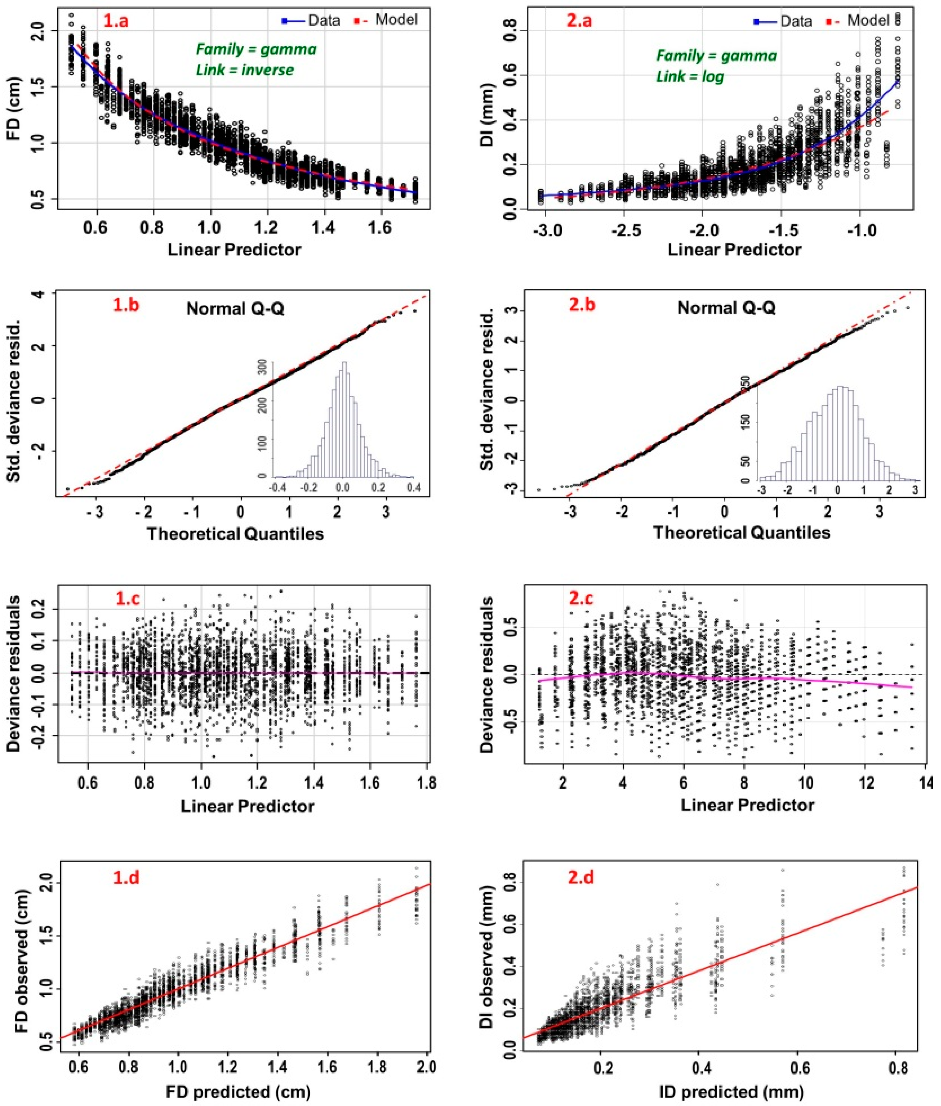
• The rest of the models were suitable, but, in accordance with the principle of parsimony, for FD, the 7 and 8 models and the Gamma model with reciprocal and log link were selected (green highlight). For ID, the Gamma log model was chosen (orange highlight).

In these models, Y = β₀ + β₁ ∗ V₁ + β_2i ∗ V_2i + β_3j ∗ V_3j + β₄ ∗ V₄ + e, where Y has a gamma distribution and uses the reciprocal for FD, and log link for ID. For FD, this model had high adjustment values (AIC = −6562, BIC = −6590, D²= 91.12 %) and, in accordance with the likelihood ratio test (p < 2.2 × 0⁻¹⁶) and the test of Wald (p < 2.2 × 10⁻¹⁶), we can assure that the model is strongly significant. Additionally, for ID, according to likelihood ratio test (p < 2.2 × 10⁻¹⁶) and the test of Wald (p < 2.2 × 10⁻¹⁶), the model is strongly significant (AIC = −9654, BIC = −9605, D² = 73.97%) with a significant and high global adjustment but smaller than FD adjustment.

3.4. Model Diagnostic

Only the most important diagnostic graphics are displayed (Figure 5) to validate the selected model.

The marginal model plots proposed by Cook and Weisberg [53] are variations on the basic residual plots, Figure 5a. These plots all have the response variable on the vertical axis, while the horizontal axis is provided in turn by each of the numeric predictors in the model and the fitted values. This marginal model can reproduce non-linear marginal relationships for the predictors. Indeed, the model, as represented by the red dashed lines, does a fairly good job of matching the marginal relationships represented by the blue solid lines. Figure 5b depicts the normal probability plots of the deviance residual. Normality (approximate normality) is in the deviance residuals, which allows us to evaluate how well satisfied the assumption of the response distribution is. This normality can be contrasted by the frequency histogram and it must fit the normal distribution. Plots of the deviance residuals against the linear predictors, Figure 5c, showed that no pattern indicates any problem with the variance function. The observed (in the y-axis) vs. predicted (in the x-axis) plot (OP), Figure 5d, is visual and immediately representative to understand the model global accuracy for both variables, FD and ID.

The estimated values for each coefficient of GLM for FD and ID, their significance and the deviations by resampling method (Bootstrap) are shown in

Table 10. The estimates of Generalized Linear Model (GLM) for footprint diameter (FD)and indentation depth (ID) with bootstrap errors.

	Model	Estimate	SE	bootBias	bootSE	t Value	Pr (>|t|)
FD	β0 (Intercept)	2.3522	0.0109	−5.04 × 104	0.0117	194.185	<2 × 10−16 ***
	β1 (V1)	−0.0255	0.0002	−1.27 × 10−6	0.0002	−128.029	<2 × 10−16 ***
	β2 (V2 Q.robur)	−0.0311	0.0030	−1.92 × 10−4	0.0047	−10.433	1.4 × 10−5 ***
	β2 (V2 E.grandis)	−0.1580	0.0024	−4.55 × 10−5	0.0050	−66.437	<2 × 10−16 ***
	β2 (V2 H.courbaril)	0.2417	0.0030	1.37 × 10−4	0.0055	79.572	<2 × 10−16 ***
	β3 (V3 EWF)	−0.0633	0.0031	−5.25 × 10−5	0.0031	39.704	<2 × 10−16 ***
	β4 (V4)	−0.2860	0.0073	3.73 × 10−4	0.0078	−39.344	<2 × 10−16 ***
ID	β0 (Intercept)	−4.0007	0.0362	−1.1 × 10−4	0.0376	−110.22	<2 × 10−16 ***
	β1 (V1)	0.0363	0.0007	−2.8 × 10−5	0.0007	53.70	<2 × 10−16 ***
	β2 (V2 Q.robur)	0.2334	0.0101	3.2 × 10−4	0.0119	22.22	<2 × 10−16 ***
	β2 (V2 E.grandis)	0.3068	0.0092	−1.1 × 10−4	0.0098	33.30	<2 × 10−16 ***
	β2 (V2 H.courbaril)	−0.5379	0.0092	−7.6 × 10−5	0.0089	−58.38	<2 × 10−16 ***
	β3 (V3 EWF)	0.0937	0.0058	3.3 × 10−4	0.0059	16.08	<2 × 10−16 ***
	β4 (V4)	0.8568	0.0261	1.1 × 10−3	0.0264	32.88	<2 × 10−16 ***

Signif. codes: 0 ‘***’; 0.001 ‘**’; 0.01 ‘*’; 0.05 ‘.’; 0.1 ‘ ’ 1.

.

FD = 2.352 − 0.026 * V1 − 0.031 * V2 _Q.robur − 0.158 * V2 _E.grandis + 0.242 * V2 _H.courbaril − 0.063 * V3 _EWF − 0.286 * V4

(1)

ID = −4.001+ 0.036 * V1 + 0.233 * V2 _Q.robur + 0.307 * V2 _E.grandis − 0.538 * V2 _H.courbaril + 0.094 * V3 _EWF + 0.857 * V4

(2)

The proportion of explained variability of the FD model (Equation (1)) is explained deviation, (Table 10) and for each of the independent variables, which we could assimilate with effect size, it is observed that “ball diameter”, 51.5%, and “species”, 28.5%, are the variables that contribute more explanation. This pattern of behavior also occurs in the ID model (Equation (2)), where there is a percentage of explanation of 23.8% for ball diameter and 31.6% for species.

The absence of collinearity was checked by the variance inflation factor (VIF) [54], which measures how much the variance of a regression coefficient is inflated due to multicollinearity in the model. The smallest possible value of VIF is one (absence of multicollinearity). As a rule of thumb, a VIF value that exceeds 5 or 10 indicates a problematic amount of collinearity [55]. In accordance with VIF of 1 or nearby of 1,

Table 11. Analysis of Deviance and Variance Inflation Factor.

	Model	Df	Deviance	AIC	Scaled Deviance	Pr (>Chi sq)	Withheld Deviance	Explained Deviance	GVIF
FD	Model null	6	22.097	−6561.4	-	-	219.913	0.909	-
	V1 (Φ ball)	1	146.829	10,429.2	16,992.6	<2.2 × 10−16 ***	124.731	0.515	1.004
	V2 (specie)	3	91.077	2829.9	9397.3	<2.2 × 10−16 ***	68.980	0.285	1.077
	V3 (floor type)	1	33.564	−5001.2	1562.2	<2.2 × 10−16 ***	11.467	0.047	1.074
	V4 (height)	1	33.486	−5011.9	1551.4	<2.2 × 10−16 ***	11.388	0.047	1.001
ID	Model null	6	286.83	−9654.0	-	-	782.11	0.732	-
	V1 (Φ ball)	1	540.90	−6885.0	2771.0	<2.2 × 10−16 ***	254.07	0.238	1.000
	V2 (specie)	3	624.50	−5977.2	3682.8	<2.2 × 10−16 ***	337.67	0.316	1.011
	V3 (floor type)	1	309.87	−9404.7	251.3	<2.2 × 10−16 ***	23.05	0.022	1.033
	V4 (height)	1	385.38	−8581.1	1074.9	<2.2 × 10−16 ***	98.56	0.092	1.000

Signif. codes: 0 ‘***’; 0.001 ‘**’; 0.01 ‘*’; 0.05 ‘.’; 0.1 ‘ ’ 1.

, the variables were not correlated (not collinear variables).

Finally, overdispersion should be accounted for in a GLM analysis. The selected FD and ID model overdispersion was checked, yielding a Pearson overdispersion value of 0.007 and 0.092, respectively, much less than 1. These values imply that the sophisticated modeling of overdispersion will be unnecessary at these very low levels [56,57].

3.5. Prediction and Validation

The model generated for FD and ID for each Φ ball × Drop height × Specie × Floor type is shown in Figure 6.

Model validation was carried out, checking the model with external bibliographic data. Almahallawi [50] worked with oak wood samples according to ASTM D2394-17 standard dropping ball of 51 mm diameter from 0.15 to 1.80 m of height, repeating test 4 for each height. The ID values for 51 mm diameter of Quercurs robur solid wood floor type compared with the proposed model line are displayed in Figure 7. The ID value variability was similar to that found in this work. Adjustment response was more acceptable than basic lineal regression (R² = 64.83% and 62.03%, respectively) and with better general adjustment in the model analysis. Likewise, this author presented oak wood samples finished with polyurethane values and he did not find differences with oak wood samples without surface treatment. Additionally, these values were consistent with his proposed model, Figure 7. In other research, Shendley [51] presented ID values to Quercus alba and Q. kelloggii with three drop heights: 0.3, 0.6 and 0.9 m. In correspondence with Quercurs robur botanical closeness, these values were included in the comparative representation. As expected, Q. alba and Q. kelloggii had similar behavior to Q. robur (Figure 7). In a similar research line, Green et al. [52] received ID values to E. globulus and Q. robur with extrapolated values of 1.80 m of height from lineal regression. These values were incorporated into this model and were consistent with it (Figure 7).

4. Conclusions

There was a greater variability of indentation depth values (ID) than in the footprint diameter (FD). For high indentation depth values, the variability is large (mean CV > 18%), while for small values, produced with low heights and small ball, the variability is very large (mean CV > 25%), yielding a response too “complacency” for E. grandis, that is, most of this group had very little response sensitivity for low values. Thus, under these conditions, it is difficult to find significant differences between groups.

The FD values were much more homogeneous, presenting a more sensitive response to the variation of the test conditions. The mean variability of the response, expressed as CV, was always below 10%. Therefore, the models established for FD were significantly more accurate than for ID and their predictions have better performance.

From these results, it is shown that fast-growing wood from E. globulus has a similar behavior to traditional hardwood species used on engineering flooring in Europe, Q. robur, and it could be a promising development in the flooring industry. However, E. grandis showed the worst values compared to traditional hardwood in all test configurations.

References

1. Andrade, A.; Jankowsky, I.P.; Takeshita, S.; Neto, P.R. Análise de qualidade em pisos de madeira. Rev. Madeira 2010, 125, 12–18. [Google Scholar]
2. Castro, G.; Zanuttini, R. Multilaminar wood: Manufacturing process and main physical-mechanical properties. Forest Prod. J. 2004, 54, 61–67. [Google Scholar]
3. Bergman, R.D.; Bowe, S.A. Life cycle inventory of manufacturing prefinished engineered wood flooring in Eastern us with comparsion to solid strip wood flooring. Wood Fiber Sci. 2011, 43, 421–441. [Google Scholar]
4. Li, N.; Tsushima, E.; Tsushima, H. Comparison of impact force attenuation by various combinations of hip protector and flooring material using a simplified fall-impact simulation device. J. Biomech. 2013, 46, 1140–1146. [Google Scholar] [CrossRef]
5. Buckley, D.S.; Clatterbuck, W.K. Proceedings of the 15th Central Hardwood Forest Conference; e-Gen. Tech. Rep. SRS–101; US Department of Agriculture, Forest Service, Southern Research Station: Knoxville, TN, USA, 2007.
6. Padilha, C.; Lima, J.T.; Silva, J.R.M.; Trugilho, P.F.; Andrade, H.B. Avaliação da qualidade da madeira de Eucalyptus urophylla para utilização em pisos. Sci. For. 2006, 71, 141–147. [Google Scholar]
7. Mania, P.; Wróblewski, M.; Wójciak, A.; Roszyk, E.; Moliński, W. Hardness of densified wood in relation to changed chemical composition. Forests 2020, 11, 506. [Google Scholar] [CrossRef]
8. Mathis, D.; Blanchet, P.; Landry, V.; Lagière, P. Impregnation of wood with microencapsulated bio-based phase change materials for high thermal mass engineered wood flooring. Appl. Sci. 2018, 8, 2696. [Google Scholar] [CrossRef] [Green Version]
9. Hague, J. Utilisation of Plantation Eucalypts in Engineered Wood Products; Forest and Wood Products Australia: Melbourne, Australia, 2013. [Google Scholar]
10. Nogueira, M.C.D.J.A.; de Araujo, V.A.; Vasconcelos, J.S.; Christoforo, A.L.; Lahr, F.A.R. Sixteen properties of Eucalyptus Tereticornis wood for structural uses. Biosci. J. 2020, 36, 449–457. [Google Scholar] [CrossRef] [Green Version]
11. Crespo, J.; Majano-Majano, A.; Lara-Bocanegra, A.J.; Guaita, M. Mechanical properties of small clear specimens of eucalyptus globulus Labill. Materials 2020, 13, 906. [Google Scholar] [CrossRef] [Green Version]
12. Derikvand, M.; Kotlarewski, N.; Lee, M.; Jiao, H.; Nolan, G. Characterisation of physical and mechanical properties of unthinned and unpruned plantation-grown eucalyptus nitens H. Deane & Maiden Lumber. Forests 2019, 10, 194. [Google Scholar] [CrossRef] [Green Version]
13. Jeon, J.Y.; Ryu, J.K.; Jeong, J.H.; Tachibana, H. Review of the impact ball in evaluating floor impact sound. Acta Acust. United Acust. 2006, 92, 777–786. [Google Scholar]
14. Todaro, L. Effect of steaming treatment on resistance to footprints in Turkey oak wood for flooring. Eur. J. Wood Prod. 2012, 70, 209–214. [Google Scholar] [CrossRef]
15. Németh, R.; Molnar, S.; Bak, M. Performance evaluation of strip parquet flooring panels after long-term, in-service exposure. Drewno 2014, 57, 1–16. [Google Scholar] [CrossRef]
16. Sepliarsky, F.; Tapias-Martin, R.; Acuña-Rello, L. Parquet multicapa de Eucalyptus globulus y Quercus robur. resistencia al impacto para diversas tipologías de fabricación. Maderas Cienc. Tecnol. 2018, 20, 103–116. [Google Scholar] [CrossRef] [Green Version]
17. Oliveira, M.B.D.; Silva, J.R.M.D.; Hein, P.R.G.; Lima, J.T. Establishment of quality classes for hardwood floorings by simulated use. CERNE 2019, 25, 105–109. [Google Scholar] [CrossRef] [Green Version]
18. Meyer, L.; Brischke, C.; Welzbacher, C.R. Dynamic and static hardness of wood: Method development and comparative studies. Int. Wood Prod. J. 2011, 2, 5–11. [Google Scholar] [CrossRef]
19. Hirata, S.; Ohta, M.; Honma, Y. Hardness distribution on wood surface. J. Wood Sci. 2001, 47, 1–7. [Google Scholar] [CrossRef]
20. Kollmann, F. Technologie des Holzes und der Holzwerkstoffe; Springer: Berlin, Germany, 1951. [Google Scholar]
21. Rautkari, L.; Kamke, F.A.; Hughes, M. Density profile relation to hardness of viscoelastic thermal compressed (VTC) wood composite. Wood Sci. Technol. 2001, 45, 693–705. [Google Scholar] [CrossRef]
22. Doyle, J.; Walker, J.C.F. Indentation of wood by wedges. Wood Sci. Technol. 1985, 19, 47–55. [Google Scholar] [CrossRef]
23. UNE-EN 1534:2020. Wood Flooring and Parquet. Detrmination of Resistance to Indentation. Test Method; Asociación Española de Normalización: Madrid, Spain, 2020. [Google Scholar]
24. ASTM D 143-14. Standard Test Methods for Small Clear Specimens of Timber; ASTM International: West Conshohocke, PA, USA, 2014. [Google Scholar]
25. Bektas, I.; Alma, M.H.; As, N. Determination of the relationships between Brinell and Janka hardness of eastern beech (Fagus orientalis Lipsky). Forest Prod. J. 2001, 51, 84. [Google Scholar]
26. Niemz, P.; Stübi, T. Investigations of hardness measurements on wood based materials using a new universal measurement system. In Proceedings of the Symposium on Wood Machining Properties of Wood and Wood Composites Related to Wood Machining, BOKU–University of Natural Resources and Applied Life Sciences, Vienna, Austria, 27–29 August 2000; pp. 51–61. [Google Scholar]
27. Heräjärvi, H. Variation of basic density and Brinell hardness within mature Finnish Betula pendula and B. pubescens stems. Wood Fiber Sci. 2004, 36, 216–227. [Google Scholar]
28. Doyle, J.; Walker, J.C.F. Indentation hardness of wood. Wood Fiber Sci. 1985, 17, 369–376. [Google Scholar]
29. Holmberg, H. Influence of grain angle on Brinell hardness of Scots pine (Pinus sylvestris L.). Holz Als Roh-Und Werkst. 2000, 58, 91–95. [Google Scholar] [CrossRef]
30. Grekin, M.I.K.A.; Verkasalo, E. Variations in and models for Brinell hardness of Scots pine wood from Finland and Sweden. Balt. For. 2013, 19, 128–136. [Google Scholar]
31. Helińska-Raczkowska, L.; Moliński, W. The effect of the Janka ball indentation depth on the hardness number determined for selected wood species. Folia For. Pol. 2003, 34, 27–36. [Google Scholar]
32. De Assis, A.A.; Alexandre, R.P.; Ballarin, A.W. Dynamic hardness of wood–measurements with an automated portable hardness tester. Holzforschung 2017, 71, 383–389. [Google Scholar] [CrossRef]
33. Ballarin, A.; Almeida, P.; Palma, H.L.; Colenci, R. Portable hardness tester for timber classification. In Proceedings of the WCTE 2010-World Conference on Timber Engineering, Riva del Garda, Italy, 20–24 June 2010; pp. 20–24. [Google Scholar]
34. UNE-408: 2011+A1:2012. Timber Structures–Structural Timber and Glued Laminated Timber. Determination of Some Physical and Mechanical Properties; Asociación Española de Normalización: Madrid, Spain, 2012. [Google Scholar]
35. EN 13183-1:2002. Moisture Content of a Piece of Sawn Timber. Part 1: Determination by Oven Dry Method; European Committee of Standardization (CEN): Brussels, Belgium, 2002. [Google Scholar]
36. ASTM D1037-99. Standard Test Methods for Evaluating Properties of Wood-Base Fiber and Particle Panel Materials; ASTM International: West Conshohocke, PA, USA, 1999. [Google Scholar]
37. AITIM. Reglamento Del Sello de Calidad Aitim Para Pavimentos de Madera, Parquet Industrial, Parquet Mosaico, Lamparquet y Tarima. 2012. Available online: http://infomadera.net/uploads/sellos_calidad/reglamento_23_Sello%204.1,%204.3%20y%204.4%20Pmosytarim_19%2007%2012.pdf (accessed on 5 December 2016).
38. Wilcox, R. Introduction to Robust Estimation and Hypothesis Testing; Academic Press: New York, NY, USA, 2016. [Google Scholar]
39. Welch, B.L. On the comparison of several mean values—An alternative approach. Biometrika 1951, 38, 330–336. [Google Scholar] [CrossRef]
40. Nelder, J.A.; Wedderburn, R.W.M. Generalized linear models. J. R. Stat. Soc. 1972, 135, 370–384. [Google Scholar]
41. Dobson, A.J. An Introduction to Generalized Linear Models; Chapman & Hall/CRC: London, UK, 2002. [Google Scholar] [CrossRef]
42. Faraway, J.J. Extending the Linear Model with R, Generalized Linear, Mixed Effects and Non-Parametric Regression Models; Chapman and Hall/CRC: New York, NY, USA, 2006. [Google Scholar]
43. Krzanowski, W.J. An Introduction to Statistical Modelling; John Wiley & Sons Inc.: London, UK, 2010. [Google Scholar]
44. Burnham, K.P.; Anderson, D.R. Model Selection and Inference: A Practical Information—Theoretic Approach; Springer: New York, NY, USA, 1998. [Google Scholar]
45. Anderson, D.R.; Burnham, K.P.; Thompson, W.L. Null hypothesis testing: Problems, prevalence, and an alternative. J. Wildl. Manag. 2000, 64, 912–923. [Google Scholar] [CrossRef]
46. Hastie, T.; Tibshirani, T.; Friedman, J. The Elements of Statistical Learning: Data Mining, Inference, and Prediction; Springer: New York, NY, USA, 2001. [Google Scholar]
47. Wackerly, D.D.; Mendenhall, W., III; Scheaffer, R.L. Mathematical Statistics with Applications; Pacific Grove, Wad worth Group, Duxbury and Brooks/Cole: London, UK, 2002. [Google Scholar]
48. Schwarz, G. Estimation the Dimension of a Model. Ann. Stat. 1978, 6, 461–464. [Google Scholar] [CrossRef]
49. Chen, J.; Chen, Z. Extended bayesian information criteria for model selection with large model space. Biometrika 2008, 95, 759–771. [Google Scholar] [CrossRef] [Green Version]
50. Almahallawi, T.M. Flooring Systems from Locally Grown Casuarina Wood: Performance Evaluation Based on Simulated in-Service Testing. Master’s Thesis, The American University in Cairo, Cairo, Egypt, 2018. [Google Scholar]
51. Shedley, P.N. The Cost Benefits of Small Log Processing Laminated Three-Ply Flooring: A Case Study in WA: A Report for the RIRDC/Land and Water Australia/FWPRDC Joint Venture Agroforestry Program and the Wood and Paper Industry Strategy-Industry Development Program; Rural Industries Research and Development Corporation: Melbourne, Australia, 2002. [Google Scholar]
52. Green, D.; von Segen, W.; Willits, S. Western Hardwoods Value-Added Research and Demonstration Program. Forest Products Laboratory; General Technical Report FPL-GTR-85; Oregon State University: Washington, DC, USA, 1995. [Google Scholar] [CrossRef]
53. Cook, R.D.; Weisberg, S. Graphics for assessing the adequacy of regression models. J. Am. Stat. Assoc. 1997, 92, 490–499. [Google Scholar] [CrossRef]
54. Fox, J.; Monette, G. Generalized collinearity diagnostics. J. Am. Stat. Assoc. 1992, 87, 178–183. [Google Scholar] [CrossRef]
55. Gareth, J.; Witten, D.; Hastie, T.; Tibshirani, R. An Introduction to Statistical Learning: With Applications in R; Springer: New York, NY, USA, 2014. [Google Scholar] [CrossRef]
56. Aitkin, M. A general maximum likelihood analysis of overdispersion in generalized linear models. Stat. Comput. 1996, 6, 251–262. [Google Scholar] [CrossRef]
57. Adewale, A.J.; Xu, X. Robust designs for generalized linear models with possible overdispersion and misspecified link functions. Comput. Stat. Data Anal. 2010, 54, 875–890. [Google Scholar] [CrossRef]
Figure 1. Impact test specimens (a) solid wood flooring (b) engineered wood flooring.
Forests 11 00933 g001
Figure 2. Device for testing dynamic hardness: 1. drop height; 2. drop support; 3. ball diameters.
Forests 11 00933 g002
Figure 3. Box plot graphics: footprint diameter (FD) for each wood specie. Different flooring types (solid wood flooring (SWF) and engineered wood flooring (EWF)), drop heights (0.60–0.75–0.90–1.05–1.20 m) and diameter balls (30–40–50mm) were represented. (a) traditional hardwood species applied on wood flooring; (b) fast-growing hardwoods.
Forests 11 00933 g003
Figure 4. Box plot graphics: indentation depth (ID) for each wood specie. Different flooring types (solid wood flooring (SWF) and engineered wood flooring (EWF)), drop heights (0.60–0.75–0.90–1.05–1.20 m) and diameter balls (30–40–50mm) were represented. (a) traditional hardwood species applied on wood flooring; (b) fast-growing hardwoods.
Forests 11 00933 g004
Figure 5. General diagnostic. 1. footprint diameter (FD); 2. indentation depth (ID); (a): Marginal model; (b): Residual normality; (c): Deviance residuals against the linear predictors; (d): Observed vs. predicted.
Forests 11 00933 g005
Figure 6. Footprint diameter (FD) and Indentation depth (ID) modelling for drop ball test for different values of the independent variables. (a) solid wood flooring (SWF); (b) engineered wood flooring (EWF).
Forests 11 00933 g006
Figure 7. Comparative representation of validation model.
Forests 11 00933 g007