Article

Reconstructing Summer Precipitation with MXD Data from Pinus sylvestris Growing in the Stockholm Archipelago

by
Eva Rocha
1,2,*,
Björn E. Gunnarson
1,2 and
Steffen Holzkämper
1,2
1
Department of Physical Geography, Stockholm University, 106 91 Stockholm, Sweden
2
Bolin Centre for Climate Research, Stockholm University, 106 91 Stockholm, Sweden
*
Author to whom correspondence should be addressed.
Atmosphere 2020, 11(8), 790; https://doi.org/10.3390/atmos11080790
Submission received: 9 June 2020 / Revised: 21 July 2020 / Accepted: 24 July 2020 / Published: 27 July 2020
(This article belongs to the Special Issue Past Climate Reconstructed from Tree Rings)

Abstract

:
Maximum latewood density (MXD) chronologies have been widely used to reconstruct summer temperature variations. Precipitation signals inferred from MXD data are, however, rather scarce. In this study, we assess the potential of using MXD data derived from Scots pine (Pinus sylvestris L.) growing in the Stockholm archipelago (Sweden) to reconstruct past precipitation variability. In this area, slow-growing pine trees emerge on flat plateaus of bedrock outcrops with thin or absent soil layers and are, therefore, sensitive to moisture variability. A 268-year-long MXD chronology was produced, and climate–growth relationships show a significant and robust correlation with May–July precipitation (PMJJ r = 0.64, p < 0.01). The MXD based May–July precipitation reconstruction covers the period 1750–2018 CE and explains 41% of the variance (r2) of the observed precipitation (1985–2018). The reconstruction suggests that the region has experienced more pluvial phases than drought conditions since the 1750s. The latter half of the 18th century was the wettest and the first half of the 19th century the driest. Climate analysis of “light rings” (LR), latewood layers of extreme low-density cells, finds their occurrence often coincides with significantly dry (<41 mm precipitation) and warmer (1–2 °C above average temperature), May–July conditions. Our analysis suggests that these extremes may be triggered by the summer North Atlantic Oscillation (SNAO).

1. Introduction

Tree-ring chronologies from high-latitudes and high-elevation sites display a strong and positive link with summer temperatures and a weak association with summer precipitation [1,2]. The opposite pattern is observed at low latitudes and elevation sites where precipitation deficits, combined with above optimal temperatures, increase plant moisture stress [2,3]. These climatic sensitivities have been used to reconstruct past temperature and moisture variability from continental to hemispherical scales [4,5,6,7,8,9]. In Scandinavia, temperature generally has a stronger influence on tree-growth than precipitation. However, positive correlations with early spring and summer precipitation are also observed [10]. Though several tree-ring width (TRW) [11,12,13], maximum latewood density (MXD) [14,15], blue intensity (BI) [16,17], and isotope [18] summer temperature reconstructions have been produced in the region, hydroclimatic studies are still scarce and have been derived from TRW data only. The few existing reconstructions are based on drought indices that include both temperature and precipitation data [19,20], or summer precipitation with a narrow seasonal window [21,22]. Recently, Seftigen et al. [23] showed the potential of using different BI derived parameters to improve hydroclimate reconstructions in the region, emphasizing the importance of wood density research in moisture-sensitive areas at high northern latitudes.
Moreover, in these areas, the landscape has been severely marked by human interference (e.g., logging and tourism), and tracts of pristine forests are rare. While it is generally accepted that ring-width data are more susceptible to abiotic disturbances, MXD data are generally considered to be less affected by the same degree of disturbance [24] and, consequently, often exhibit a stronger climatic signal [25], leading to more robust climatic reconstructions.
In the present study, we develop a seasonal precipitation reconstruction from the Stockholm archipelago based on Scots pine (Pinus sylvestris L.) maximum latewood density data and compared it with its corresponding TRW to analyze the climatic signal. Furthermore, we assessed the potential of using light rings (LR) as a bioindicator of extreme climatic conditions in the study region.
Light rings are characterized by a few layers of thin-walled latewood cells [26]; they are light-colored and, therefore, easily recognizable under the microscope. LR occurrence is mainly related to cambial activity and latewood formation and can, therefore, provide important information on climate–growth conditions during the growing season [27,28,29]. In regions where tree-growth is mostly controlled by temperature, light rings occurrence is mainly associated with cold conditions during the growing season. Very few studies have assessed the occurrence of light rings in trees growing under moisture limiting conditions [30].
The main objectives of this study are (1) to assess the climate–growth relationship in a precipitation sensitive area, (2) to consider the spatiotemporal representation of this new reconstruction, and (3) to assess the relationship between LR and local climatic factors.

2. Materials and Methods
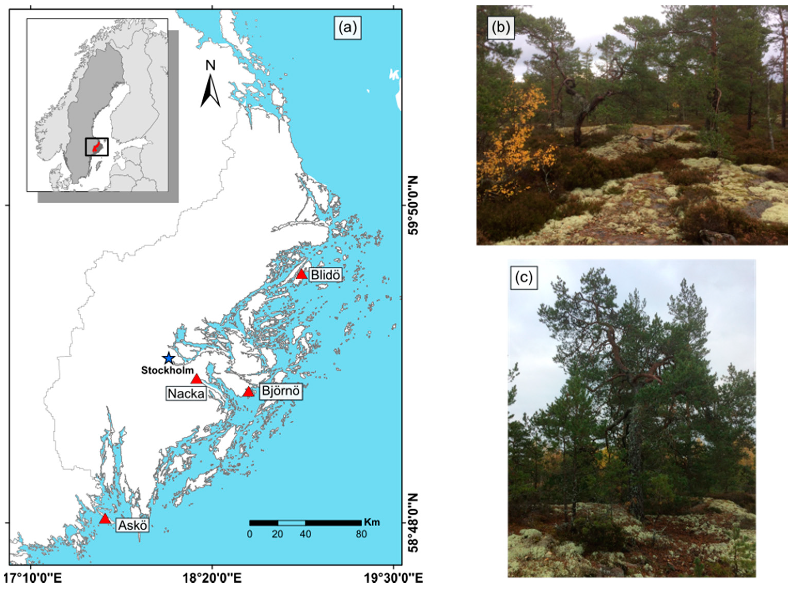
2.1. Study Area

The study area ranges between 58°49′–59°39′ N and 17°38′–18°34′ E in the Stockholm archipelago, located on the east coast of Sweden (Figure 1). The annual mean temperature in the region is 6.6 °C (Stockholm meteorological station, period 1981–2010). February, in general, is the coldest month with a mean temperature of −3.0 °C and July the warmest with a mean temperature of 17.2 °C. The mean annual precipitation is 539 mm with peak rainfall occurring in July and August, and the length of the growing season is 180 days (Swedish Meteorological and Hydrological Institute, SMHI). Additionally, summer precipitation (May–July) was found to be inversely related to temperature (r = −0.35; p < 0.01). The vegetation belongs to the boreonemoral zone, characterized by mixed forests, including P. sylvestris, Picea abies, Quercus robur, Betula pendula, and Populus tremula [31]. The isostatic uplift in the region (4 mm/year) creates a peculiar type of forest known as flat rock forests (Sw: Hällmarksskog). As new land surfaces are exposed to rebound wave action barren bedrock outcrops are left behind. In time, as uplift progresses and these new islands rise above the wave action, they begin to accumulate a very thin layer of dry, nutrient-poor soil, that can support a thin cover of vegetation consisting mainly of mosses and lichen, and slow-growing pine trees emerging from soil-filled cracks in the bedrock. These island forests are not easily accessible and have low economic value. Consequently, the trees can be several hundred years old.

2.2. Tree-Ring Data

Scots pine tree-ring samples were collected from living trees growing in drought-prone environments (Figure 1), where tree-growth is predominantly limited by moisture availability [32]. The locations are the Askö nature reserve, the southernmost site in the study region; the Nacka and Björnö nature reserves, in the central part of the archipelago; and Blidö, the northernmost site in the study area. Tree-cores were collected at breast height (ca 1.3 m above the ground), using a Swedish increment borer (Ø10 mm). Annual ring widths were measured with an accuracy of ±1 µm using a sliding measuring table connected to the TSAP-Win software from Rinntech.
The radiodensitometric data were produced at the Stockholm tree-ring laboratory using the ITRAX-multiscanner from Cox Analytical Systems (www.coxsys.se) and the cores prepared according to standard techniques [33]. Tree cores were glued onto strips of wood, and thin laths (1.2 mm thick) were cut using a twin bladed circular saw. To extract resins and other compounds that are not related to the wood density but may interfere with the analysis, the laths were treated for 24 h with alcohol in a Soxhlet. The samples were then acclimatized in a room with controlled temperature (20 °C) and relative humidity (50%) and once environmentally equilibrated X-ray exposed in the ITRAX- multiscanner equipped with a chrome (Cr) tube, regulated at 30 kV and 50 mA with a line scanning step size of 20 μm for 75 ms [15]. The ITRAX-scan produces an optical digital image and a 16-bit grayscale radiographic image with a resolution of 1270 dpi. The grey levels were calibrated using a calibration wedge from Walesch Electronic GmbH. Density data were produced from the radiographic images with WinDENDRO (Régent Instruments Canada Inc., version 2017a).

2.3. Data Analysis

2.3.1. Standardization and Statistical Analysis

The individual tree-ring series were tested for cross-dating accuracy using the COFECHA software [34], and the four sites were averaged into one single regional chronology.
To remove non-climatic trends related to tree-age, size and stand dynamics [35,36], the data were standardized using the ARSTAN [37]. The density data were characterized by a positive growth trend over the juvenile period and a negative trend thereafter. For this reason, standardization was performed by fitting a Hugershoff-growth curve [38,39] to each density series. The TRW data were standardized by fitting an age-dependent smoothing spline individually to each series. The strength of the chronology was assessed through the inter-series correlation (Rbar), representing the degree of coherence between the density series, and the expressed population signal (EPS: calculated using 50-year window and 25-year lags), which is a measure of the degree to which the mean of all series represents a hypothetically perfect chronology [40,41].

2.3.2. Climate Data

Instrumental data were obtained from the Stockholm meteorological station (59.20.52° N, 18.3.45° E; SMHI), including monthly mean temperature (1895–2018 CE) and monthly precipitation sums (1895–2018 CE). Bootstrapped correlations were generated from 1000 simulations computed with SPSS (SPSS version 26.0, Chicago, IL, USA) to identify and evaluate the climatic signal in the standardized MXD chronology. The spatial correlations between the MXD chronology and 0.5° gridded CRU TS 4.03 climate data obtained from the Climate Research Unit [42] for the period 1901–2018 were produced by KNMI’s climate explorer [43].

2.3.3. Precipitation Reconstruction

The standard MXD chronology and the instrumental precipitation data from Stockholm were used to develop a simple linear regression transfer function to reconstruct past summer precipitation in the region [32]. The mean of May–July was preferred over total precipitation as a predictand since it led to lower standard errors. The MXD chronology was used as the predictor. The robustness of the reconstruction was assessed by the split-sample calibration-validation method. The instrumental period was divided into equal-length calibration and verification periods (i.e., 1895–1956 and 1957–2018) and validation statistics, those recommended by the National Research Council [44], were computed. These included the squared correlation coefficient (r2), reduction of error (RE), and coefficient of efficiency (CE). The verification and calibration periods were then switched, and the validation statistics repeated.
To identify years of anomalously dry and wet conditions in the reconstruction, thresholds were determined based on the percentile distribution of the precipitation levels for the entire 1750–2018 period. Dry summer years were considered as those when precipitation values were below the 15th percentile (<41 mm), and wet summer years when precipitation values were above the 85th percentile (>61 mm). When summer precipitation sums exceeded or fell below the average (51 mm) for 3 or more consecutive years, the period was labeled wet or dry, accordingly. Finally, to place the present reconstruction in a spatial context, it was compared against an existent TRW hydroclimatic reconstruction from Scandinavia (henceforth ScandH17) [20]. The two reconstructions shared no common predictors. The ScandH17 record represents a regional standardized precipitation evapotranspiration index (SPEI) [45] reconstruction, targeting June SPEI, aggregated over a 2-month timescale. Both reconstructions were z-scored over the common period 1750–1995.

2.3.4. Light Ring Formation Years

Light rings were first identified by calculating the mean and standard deviation of each latewood density series then, following the methodology outlined in Wang et al. [29], all data were divided into three groups: weak light rings (when the maximum latewood density of a ring was lower than one standard deviation below the series mean), medium light rings (when the maximum latewood density of a ring was lower than one and a half standard deviations below the series mean) and strong light rings (when the maximum latewood density of a ring was lower than two standard deviations below the series mean). A final chronology, including LRs of all magnitudes, was developed with those years where at least 30% of the trees in the composite chronology presented such a decline in the latewood density. The light ring’s climate–growth relationship was assessed by the non-parametric Mann–Whitney U-test statistics over the period 1895–2018. In this approach, LR years and normal years (NY) were divided into two groups, and the Mann–Whitney U-test used to compare differences in the means of monthly precipitation and temperature of the two groups. A composite map of May–July 500-hPa geopotential heights (Twentieth Century Reanalysis Project V2) [46] was generated in KNMI climate explorer, to evaluate the relationship between the occurrence of LR years and atmospheric circulation regimes over the period 1838–2015.

3. Results

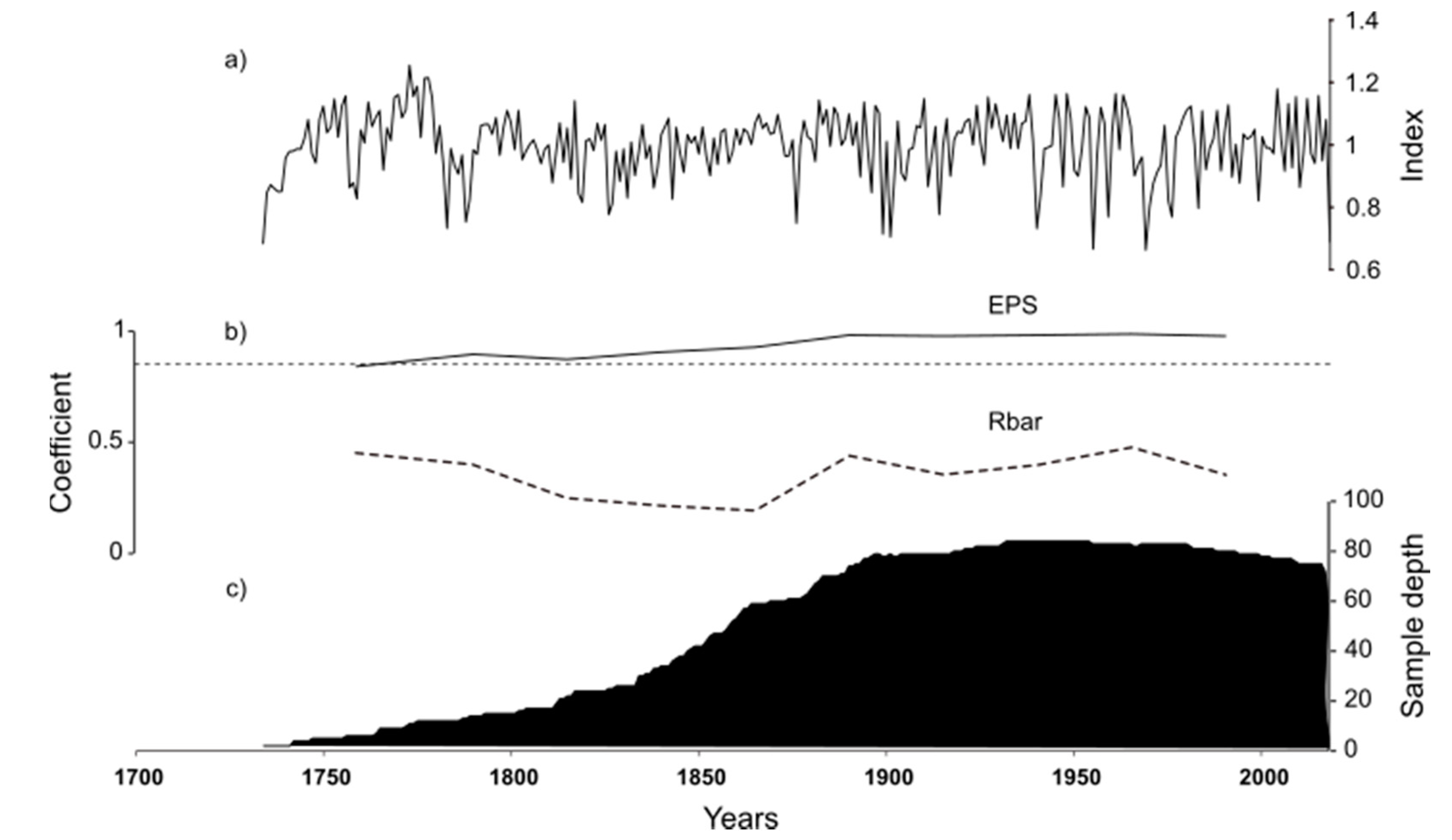
3.1. Chronology Characteristics

Four site chronologies were developed from the study area and averaged into a composite chronology containing a total of 90 density series. Within sites, the series intercorrelation varied from 0.55 for Blidö, the northernmost site, to 0.69 for Nacka nature reserve, highlighting the importance of sample replication (Table 1). The oldest forest stand was found at the Björnö nature reserve, where the oldest tree was 286 years old. The youngest forest stand was found at Blidö, where the oldest tree was 192 years old (Table 1).
The final composite chronology from the Stockholm archipelago spans the period 1734 to 2018 CE (Figure 2). The average tree age was 158 years and displayed a mean sensitivity of 0.17. Accepted EPS values (≥0.85) were reached after 1750 CE when sample depth was ≥5 samples (Figure 2), and, therefore, precipitation was reconstructed from 1750 to 2018 CE.

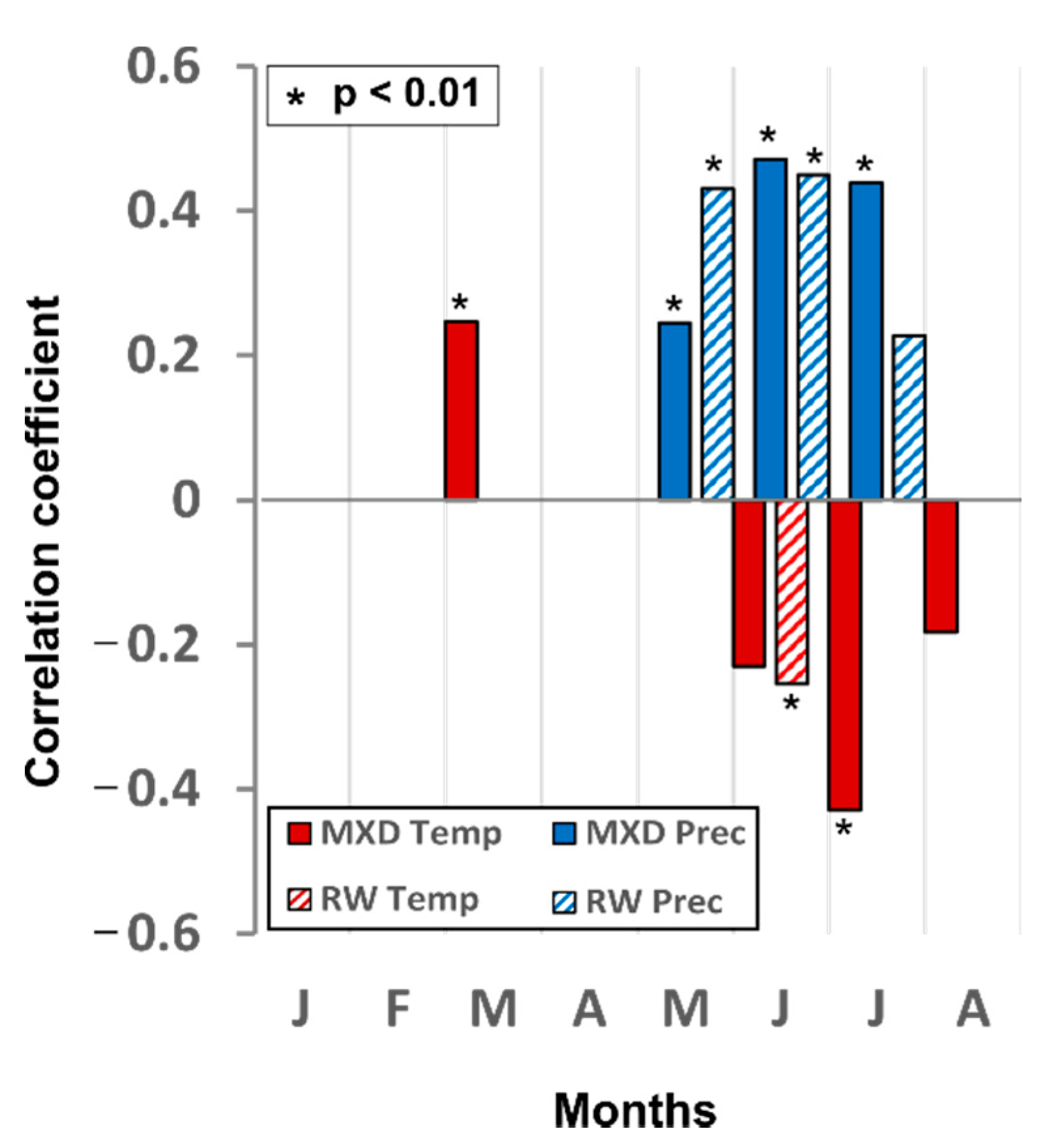
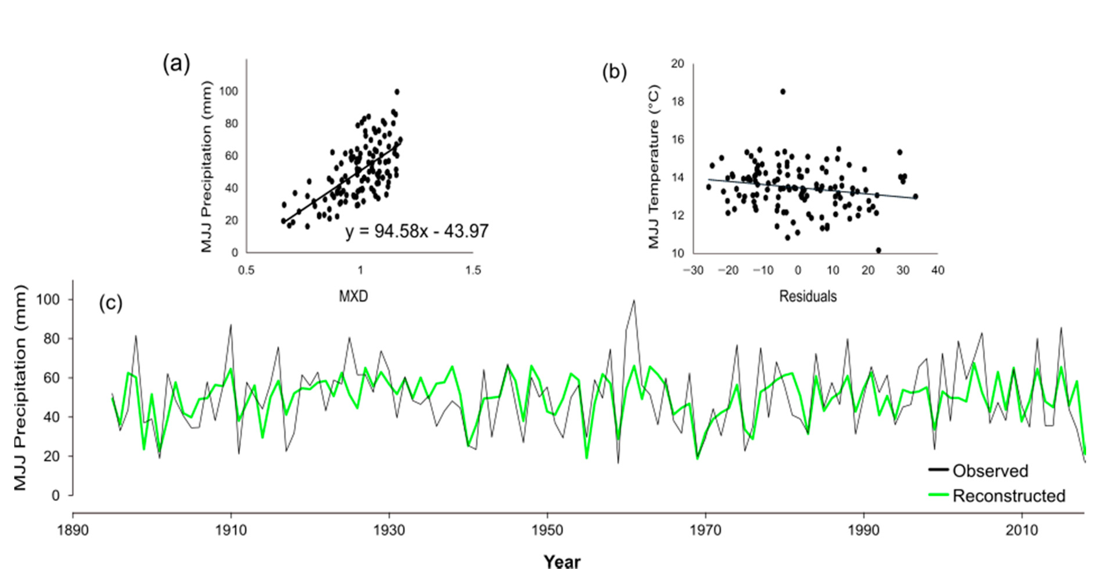
3.2. Climate Sensitivity

Climate growth analysis shows a significant (p < 0.01) and positive response of Scots pine trees to summer (May–July) precipitation (r = 0.64) (Figure 3) with the highest association found in June (r = 0.47). In contrast to precipitation, significant (p < 0.01) negative correlations were found for July temperature (r = −0.37). While the previous year’s temperature did not influence density formation, a weak and positive response (r = 0.20; p < 0.05) was found with the previous year’s August precipitation.
Spatial correlation analysis between the MXD chronology and gridded May–July precipitation data showed a strong positive correlation (r ≈ 0.6) centered over east-central Sweden. Significant, though weaker correlations extended west into Norway and southeast into Lithuania, Latvia, and Estonia (Figure 4).

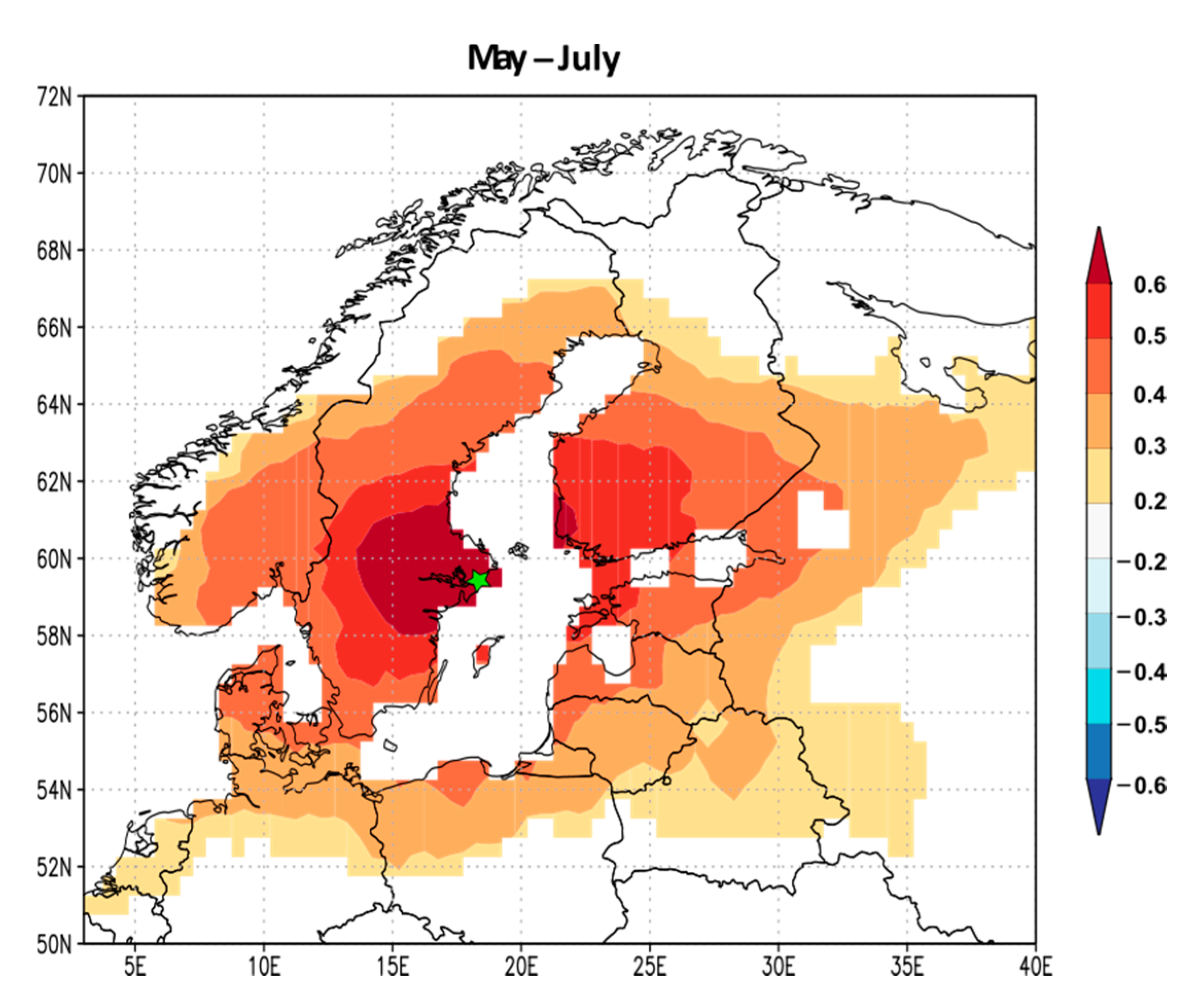
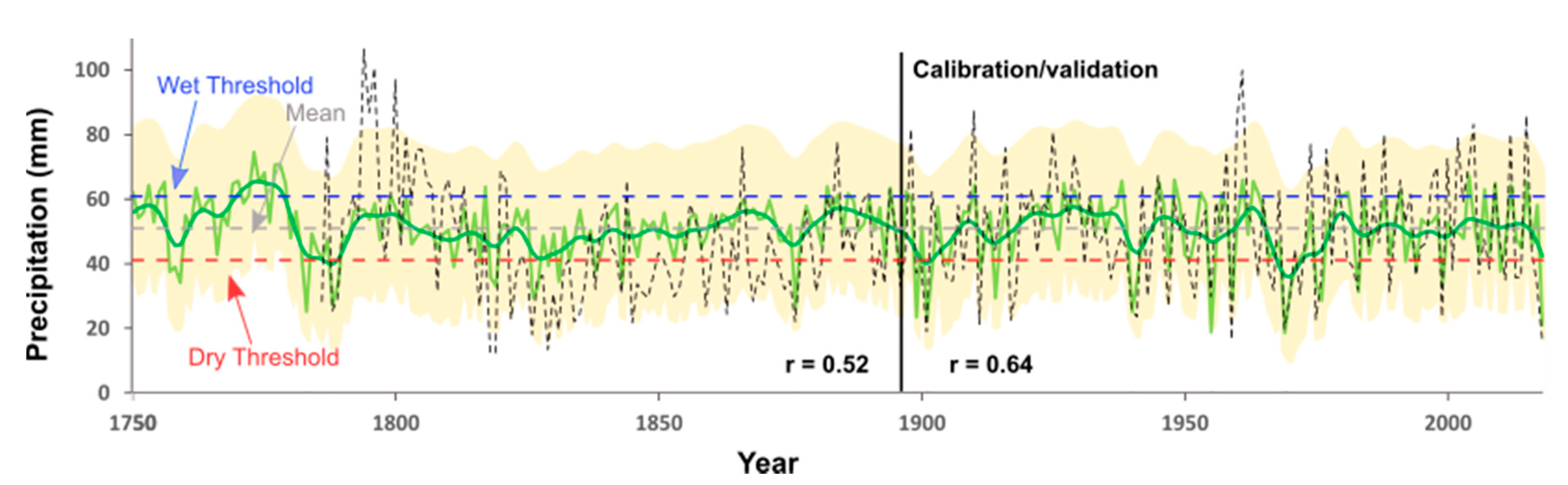
3.3. Regional Summer Precipitation Reconstruction

Based on the climate-sensitivity analysis, a transfer function using a linear regression model was developed to estimate May–July precipitation. The regression equation obtained for the period 1985–2018 was P MJJ(t) = −43.9 + 94.5MXD(t). The calibration and verification of split period statistics confirm the reliability of the model to predict the observed summer precipitation variability. The positive CE and RE statistics indicate the strength of the model. A weak negative (r ≈ −0.2, p < 0.05) correlation was found between the regression residuals and May–July temperature. The calibration and verification statistics are shown in Table 2. The final reconstruction model accounted for 41% of the variance in the instrumental May–July precipitation (Figure 5). The full reconstruction contained 41 dry (<41 mm) and 40 wet (>61 mm) years, out of which 18 dry and 19 wet were recorded in pre-instrumental years (1750–1894) (Figure 6).
The highest cluster of wet years occurred in the latter half of the 18th century. In contrast, the early 19th century presented the highest cluster of dry years (Figure 6). The driest pre-instrumental year was found in 1783 (25.4 mm), whereas the wettest was in 1773 (74.7 mm). Analysis of the reconstructed summer precipitation in pre-instrumental years indicated several periods of dry and wet conditions in the region (Figure 6). The most prolonged period of dryness started in 1782 and lasted for 10 consecutive years, whereas the most prolonged period of wetness started in 1767 and lasted for 13 consecutive years.

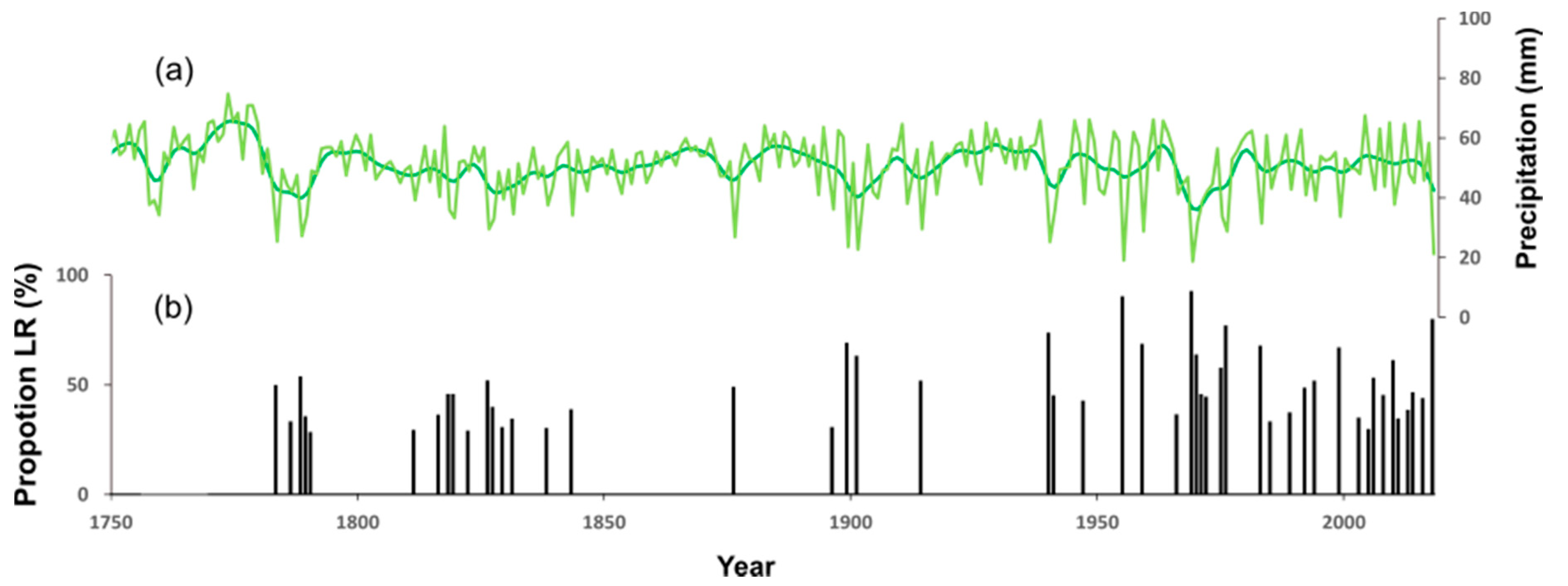
3.4. Light Ring Chronology
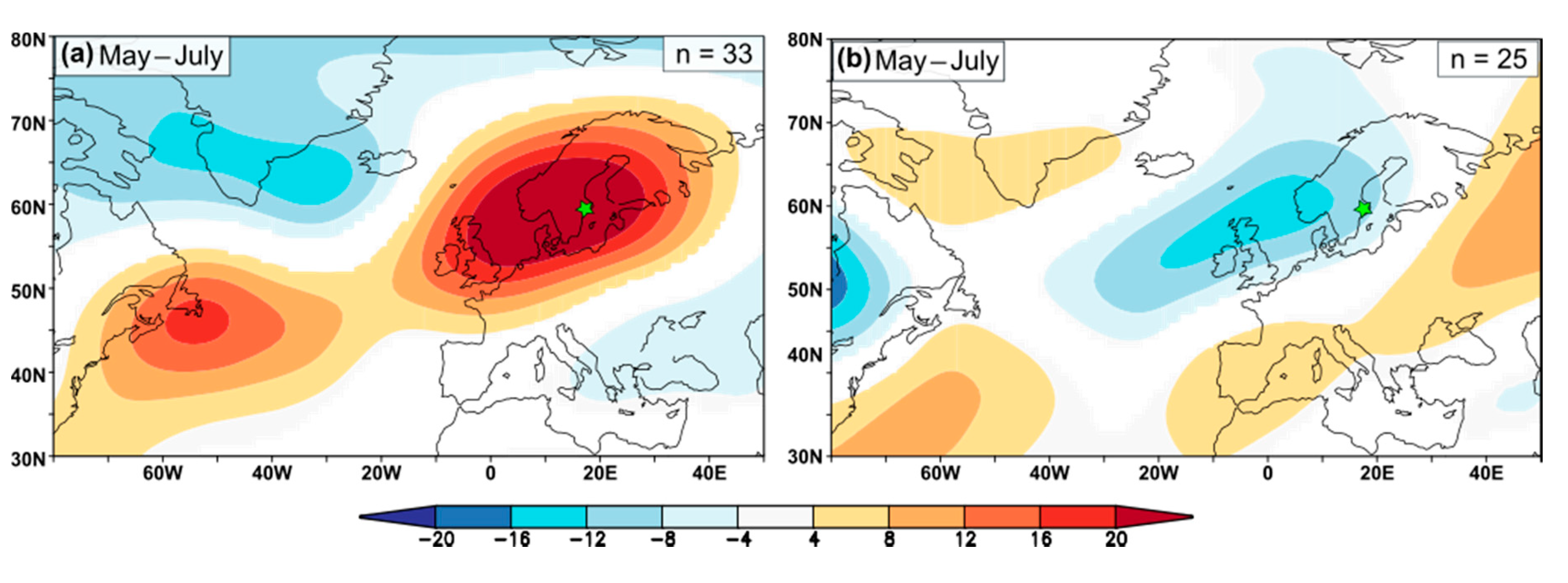
The final LR chronology from the archipelago covers the period 1783–2018 CE, with a total of 47 LR years identified that meet the >30% threshold (Figure 7). The early 19th century and the second half of the 20th century contain the highest occurrence of LR years, with 10 and 16, respectively. The climate–growth/-light ring analysis, conducted over the instrumental period (1895–2018), revealed that the frequency of LR is associated with years in which the total precipitation in May, June, and July was significantly low (p < 0.01). Significant differences were also observed for the monthly mean temperatures of May, June, July, and August (Table 3). Analysis of the 500-hPa geopotential height composite map of all LR years, over the period 1838–2015, suggested that LR occurrence was also associated with persistent positive height anomalies during summer (May–July) centered over the British Isles and northwestern Europe extending west into eastern Canada (Figure 8a).

4. Discussion

The final MXD reconstruction from the archipelago can explain 41% of the total variance in the instrumental May–July precipitation data from Stockholm, which is an improvement in comparison to the 30% (May–June) in Linderholm et al. [47]. In 2013, Seftigen et al. [48] presented a more robust result by using a network of moisture-sensitive chronologies calibrated against standardized precipitation index (SPI), capturing 41.6% of the total variance in the instrumental data, however, with a shorter response window (June–July).
Comparison between the MXD and the TRW chronologies from the archipelago show a reasonably good agreement on the interannual timescale (r = 0.7, n = 269, p < 0.01). The climatic signal was more pronounced for the MXD parameter (Figure 3), and our results showed that, in comparison to TRW, MXD data can improve the precipitation signal and extend the target window for seasonal reconstructions (Table 2), similar to what has been reported several times before for temperature [14,15,25,49,50]. However, since precipitation is highly variable in space and time, a reduced agreement between the predictors and the instrumental data is expected, and, therefore, our reconstruction only account for less than half of the variance in the instrumental May–July precipitation.
Although requiring fewer samples to produce robust paleoclimatic reconstructions, a decrease in variance was observed between ca. 1800 and 1870 in the MXD data, likely due to a lower coherence between the density series, as shown by the EPS and Rbar statistics (Figure 2). It is important to highlight that the period between 1806 and 1835 is reported as one of the longest continuous droughts in the region [51], and the lower agreement between the series may be caused by the experienced physiological stress.
To set the chronology into a spatial context, it was compared against the TRW hydroclimate (SPEI) reconstruction from Scandinavia (ScandH17) [20]. Despite the different seasonal target and slightly different calibration period (i.e., 1901–1995), correlations over the common period 1750–2018 point to a good coherence between the records on the interannual timescale (r = 0.48, n = 246, p < 0.01) (Figure 9). However, the MXD chronology seemed to capture better the severity of the extreme precipitation deficits than the TRW ScandH17 chronology. Similar findings were reported by Esper et al. [52] for temperature cooling estimates of post-volcanic eruptions. Another interesting observation is the increased variability displayed by the MXD data from ca. 1940 CE onwards. Analysis of the precipitation record from Stockholm showed that, during the 2nd half of the 20th century, dry and wet summers were not only more frequent but also more interspersed. The biological memory imprinted in the TRW data, reflecting previous year conditions [52,53], may reduce the ability of this proxy to represent interannual variability, suggesting a better fitting of the MXD data as a proxy for short-term climatic variations [25]. On the interdecadal timescale, similarities among the records were more pronounced during dry periods. The largest discrepancy in the reconstructions was found between 1768 and 1777 CE. The narrow seasonal target, together with the slightly different calibration period (i.e., 1901–1995), may explain the overall higher mean of the ScandH17 in the 20th century.
The climate/growth analysis indicated a weaker response of the MXD proxy to May precipitation (r = 0.24), reflecting the period of earlywood formation [23]. The strong climatic response observed between MXD and June–July precipitation (r = 0.47 and r = 0.44, respectively) showed that increased late summer precipitation in the region may lead to prolonged cell maturation (i.e., thicker cell walls), increased density [54], and probably result in an extended growing season. Our data also showed that precipitation deficit generated low MXD values, mainly due to the slow cell wall thickening of the latewood cells [32]. This process originated from light-colored rings, characterized by very few layers of latewood cells [26,29]. Our results showed that the observed light rings in the archipelago chronology are not only a product of precipitation deficit but also of above-average summer temperatures (1 to 2 °C), especially in July. Higher temperatures lead to higher evaporation rates directly affecting tree-growth in moisture sensitive areas. To withstand extreme drought events and prevent hydraulic failure, trees close their stomata, thereby limiting photosynthesis and cell enlargement [55,56] that may result in the formation of light rings [30]. Most light ring research has been conducted in regions where annual tree growth is limited by temperature, strongly suggesting low thermal conditions during latewood formation as the main reasons for light ring formation [27,28,57,58]. Here we showed that light rings can also be used in moisture sensitive regions as a bioindicator of extreme drought conditions. Similar findings were reported by Liang and Eckstein [30] for semiarid areas. As such studies are still scarce, complementary cellular analysis using micro-coring or pinning [59,60] would help to better understand the relationship between climate and light ring formation years.
Atmospheric synoptic conditions during light ring years (Figure 8a) resembled the pattern as described for the positive phase of the summer North Atlantic Oscillation (SNAO); a dipole pressure field further characterized by warm and dry conditions over northern Europe and cold anomalies over Greenland [61]. In contrast, during reconstructed wet years (Figure 8b), synoptic conditions resembled the negative phase of the SNAO, where a southward displacement of the main storm track leads to increased precipitation and cooler conditions over the British Isles and southern Scandinavia [62,63]. This analysis highlights the influence of large-scale circulation patterns on Scandinavian regional climate.

5. Conclusions

In this study, we presented a new precipitation reconstruction for east-central Sweden derived from MXD data. The reconstruction spanned the period 1750 to 2018 CE and captured 41% of the variance in the instrumental record. Our results showed that MXD provides a stronger climate–growth relationship than TRW and allows a wider target seasonal average (May–July) to be reconstructed. The reconstruction showed that the driest pre-instrumental period occurred in the 1780s–1790s and the two wettest in the late 1760s–1780s and 1860s early 1870s. The developed light-ring chronology can be used to assess the impact of large-scale circulation patterns on regional climate variability.
Several dendroclimatic studies from central and southern Scandinavia have shown the potential of using Scots pine TRW data to reconstruct past moisture availability. The addition of this new dataset to the existent network of moisture sensitivity chronologies is an important achievement towards a more robust understanding of past climate variability in the region. The combination of different tree-ring parameters, such as TRW, MXD, and LR, provides seasonal information and is the key to continue improving our knowledge on past climatic systems at the regional scale.

Author Contributions

E.R., B.E.G. and S.H. designed the study. E.R., B.E.G. and S.H. conducted field and laboratory work. Data were analyzed by E.R, and all authors discussed the results and contributed to the final manuscript. All authors have read and agreed to the published version of the manuscript.

Funding

This research was supported by the Bolin Centre for Climate Research.

Acknowledgments

Support for the Twentieth Century Reanalysis Project version 3 dataset is provided by the U.S. Department of Energy, Office of Science Biological and Environmental Research (BER), by the National Oceanic and Atmospheric Administration Climate Program Office, and by the NOAA Earth System Research Laboratories Physical Sciences Laboratory.

Conflicts of Interest

The authors declare no conflict of interest.

References

  1. Linderholm, H.W.; Nicolle, M.; Francus, P.; Gajewski, K.; Helama, S.; Korhola, A.; Solomina, O.; Yu, Z.; Zhang, P.; D’Andrea, W.J.; et al. Arctic hydroclimate variability during the last 2000 years: Current understanding and research challenges. Clim. Past 2018, 14, 473–514. [Google Scholar] [CrossRef] [Green Version]
  2. St. George, S. An overview of tree-ring width records across the Northern Hemisphere. Quat. Sci. Rev. 2014, 95, 132–150. [Google Scholar] [CrossRef]
  3. St. George, S.; Ault, T.R. The imprint of climate within Northern Hemisphere trees. Quat. Sci. Rev. 2014, 89, 1–4. [Google Scholar] [CrossRef]
  4. Cook, E.R.; Seager, R.; Kushnir, Y.; Briffa, K.R.; Büntgen, U.; Frank, D.; Krusic, P.J.; Tegel, W.; van der Schrier, G.; Andreu-Hayles, L.; et al. Old World megadroughts and pluvials during the Common Era. Sci. Adv. 2015, 1, e1500561. [Google Scholar] [CrossRef] [Green Version]
  5. Cook, E.R.; Meko, D.M.; Stahle, D.W.; Cleaveland, M.K. Drought Reconstructions for the Continental United States. J. Clim. 1999, 12, 1145–1162. [Google Scholar] [CrossRef] [Green Version]
  6. D’Arrigo, R.; Wilson, R.; Jacoby, G. On the long-term context for late twentieth century warming. J. Geophys. Res. Atmos. 2006, 111. [Google Scholar] [CrossRef]
  7. Schneider, L.; Smerdon, J.E.; Büntgen, U.; Wilson, R.J.S.; Myglan, V.S.; Kirdyanov, A.V.; Esper, J. Revising midlatitude summer temperatures back to A.D. 600 based on a wood density network. Geophys. Res. Lett. 2015, 42, 4556–4562. [Google Scholar] [CrossRef] [Green Version]
  8. Stoffel, M.; Khodri, M.; Corona, C.; Guillet, S.; Poulain, V.; Bekki, S.; Guiot, J.; Luckman, B.H.; Oppenheimer, C.; Lebas, N.; et al. Estimates of volcanic-induced cooling in the Northern Hemisphere over the past 1500 years. Nat. Geosci. 2015, 8, 784–788. [Google Scholar] [CrossRef]
  9. Wilson, R.; D’Arrigo, R.; Buckley, B.; Büntgen, U.; Esper, J.; Frank, D.; Luckman, B.; Payette, S.; Vose, R.; Youngblut, D. A matter of divergence: Tracking recent warming at hemispheric scales using tree ring data. J. Geophys. Res. Atmos. 2007, 112. [Google Scholar] [CrossRef] [Green Version]
  10. Linderholm, H.W.; Björklund, J.A.; Seftigen, K.; Gunnarson, B.E.; Grudd, H.; Jeong, J.-H.; Drobyshev, I.; Liu, Y. Dendroclimatology in Fennoscandia—From past accomplishments to future potential. Clim. Past 2010, 6, 93–114. [Google Scholar] [CrossRef] [Green Version]
  11. Briffa, K.R.; Bartholin, T.S.; Eckstein, D.; Jones, P.D.; Karlén, W.; Schweingruber, F.H.; Zetterberg, P.A. 1400-year tree-ring record of summer temperatures in Fennoscandia. Nature 1990, 346, 434–439. [Google Scholar] [CrossRef]
  12. Helama, S.; Lindholm, M.; Timonen, M.; Meriläinen, J.; Eronen, M. The supra-long Scots pine tree-ring record for Finnish Lapland: Part 2, interannual to centennial variability in summer temperatures for 7500 years. Holocene 2002, 12, 681–687. [Google Scholar] [CrossRef]
  13. Linderholm, H.W.; Gunnarson, B.E. Summer Temperature Variability in Central Scandinavia during the Last 3600 Years. Geogr. Ann. Ser. A Phys. Geogr. 2005, 87, 231–241. [Google Scholar] [CrossRef]
  14. Grudd, H. Torneträsk tree-ring width and density ad 500–2004: A test of climatic sensitivity and a new 1500-year reconstruction of north Fennoscandian summers. Clim. Dyn. 2008, 31, 843–857. [Google Scholar] [CrossRef] [Green Version]
  15. Gunnarson, B.; Linderholm, H.; Moberg, A. Improving a tree-ring reconstruction from west-central Scandinavia: 900 years of warm-season temperatures. Clim. Dyn. 2011, 36, 97–108. [Google Scholar] [CrossRef]
  16. Björklund, J.A.; Gunnarson, B.E.; Seftigen, K.; Esper, J.; Linderholm, H.W. Blue intensity and density from northern Fennoscandian tree rings, exploring the potential to improve summer temperature reconstructions with earlywood information. Clim. Past 2014, 10, 877–885. [Google Scholar] [CrossRef] [Green Version]
  17. Fuentes, M.; Salo, R.; Björklund, J.; Seftigen, K.; Zhang, P.; Gunnarson, B.; Aravena, J.-C.; Linderholm, H.W.A. 970-year-long summer temperature reconstruction from Rogen, west-central Sweden, based on blue intensity from tree rings. Holocene 2018, 28, 254–266. [Google Scholar] [CrossRef] [Green Version]
  18. Loader, N.J.; Young, G.H.F.; Grudd, H.; McCarroll, D. Stable carbon isotopes from Torneträsk, northern Sweden provide a millennial length reconstruction of summer sunshine and its relationship to Arctic circulation. Quat. Sci. Rev. 2013, 62, 97–113. [Google Scholar] [CrossRef]
  19. Drobyshev, I.; Niklasson, M.; Linderholm, H.W.; Seftigen, K.; Hickler, T.; Eggertsson, O. Reconstruction of a regional drought index in southern Sweden since AD 1750. Holocene 2011, 21, 667–679. [Google Scholar] [CrossRef]
  20. Seftigen, K.; Goosse, H.; Klein, F.; Chen, D. Hydroclimate variability in Scandinavia over the last millennium—Insights from a climate model-proxy data comparison. Clim. Past 2017, 13, 1831–1850. [Google Scholar] [CrossRef] [Green Version]
  21. Helama, S.; Lindholm, M. Droughts and rainfall in south-eastern Finland since AD 874, inferred from Scots pine ring-widths. Boreal Environ. Res. 2003, 8, 171–183. [Google Scholar]
  22. Jönsson, K.; Nilsson, C. Scots Pine (pinus sylvestris L.) on Shingle Fields: A Dendrochronologic Reconstruction of Early Summer Precipitation in Mideast Sweden. J. Clim. 2009, 22, 4710–4722. [Google Scholar] [CrossRef] [Green Version]
  23. Seftigen, K.; Fuentes, M.; Ljungqvist, F.C.; Björklund, J. Using Blue Intensity from drought-sensitive Pinus sylvestris in Fennoscandia to improve reconstruction of past hydroclimate variability. Clim. Dyn. 2020. [Google Scholar] [CrossRef]
  24. Rydval, M.; Druckenbrod, D.; Anchukaitis, K.J.; Wilson, R. Detection and removal of disturbance trends in tree-ring series for dendroclimatology. Can. J. For. Res. 2016. [Google Scholar] [CrossRef] [Green Version]
  25. Wilson, R.; Anchukaitis, K.; Briffa, K.R.; Büntgen, U.; Cook, E.; D’Arrigo, R.; Davi, N.; Esper, J.; Frank, D.; Gunnarson, B.; et al. Last millennium northern hemisphere summer temperatures from tree rings: Part I: The long term context. Quat. Sci. Rev. 2016, 134, 1–18. [Google Scholar] [CrossRef] [Green Version]
  26. Filion, L.; Payette, S.; Gauthier, L.; Boutin, Y. Light rings in subarctic conifers as a dendrochronological tool. Quat. Res. 1986, 26, 272–279. [Google Scholar] [CrossRef]
  27. Girardin, M.P.; Tardif, J.C.; Epp, B.; Conciatori, F. Frequency of cool summers in interior North America over the past three centuries. Geophys. Res. Lett. 2009, 36. [Google Scholar] [CrossRef]
  28. Tardif, J.C.; Girardin, M.P.; Conciatori, F. Light rings as bioindicators of climate change in Interior North America. Glob. Planet. Chang. 2011, 79, 134–144. [Google Scholar] [CrossRef]
  29. Wang, L.; Payette, S.; Bégin, Y.A. Quantitative Definition of Light Rings in Black Spruce (Picea mariana) at the Arctic Treeline in Northern Québec, Canada. Arct. Antarct. Alp. Res. 2000, 32, 324–330. [Google Scholar] [CrossRef]
  30. Liang, E.; Eckstein, D. Light rings in Chinese pine (Pinus tabulaeformis) in semiarid areas of north China and their palaeo-climatological potential. New Phytol. 2006, 171, 783–791. [Google Scholar] [CrossRef]
  31. Rydin, H.; Snoeijs, P.; Diekmann, M.; Van Der Maarel, E. (Eds.) Swedish Plant Geography (Acta Phytogeographica Suecica); Svenska Växtgeografiska Sällskapet: Uppsala, Sweden, 1999; ISBN 978-91-7210-484-6. [Google Scholar]
  32. Fritts, H.C. Tree Rings and Climate; Academic Press: Cambridge, MA, USA, 1976; ISBN 978-0-12-268450-0. [Google Scholar]
  33. Schweingruber, F.H.; Fritts, H.C.; Bräker, O.U.; Drew, L.G.; Schär, E. The X-Ray Technique as Applied to Dendroclimatology. Tree-Ring Bull. 1978, 38, 61–91. [Google Scholar]
  34. Holmes, R.L. Computer-Assisted Quality Control in Tree-Ring Dating and Measurement. Tree-Ring Bull. 1983, 43, 69–78. [Google Scholar]
  35. Fritts, H.C.; Guiot, J.; Gordon, G.A.; Schweingruber, F. Methods of Calibration, Verification, and Reconstruction. In Methods of Dendrochronology: Applications in the Environmental Sciences; Cook, E.R., Kairiukstis, L.A., Eds.; Springer: Dordrecht, The Netherlands, 1990; pp. 163–217. ISBN 978-94-015-7879-0. [Google Scholar]
  36. Schweingruber, F.H. Tree Rings and Environment: Dendroecology; Paul Haupt AG: Berne, Switzerland, 1996; p. 609. [Google Scholar]
  37. Cook, E.R.; Krusic, P.J. Program ARSTAN: A Tree-Ring Standardization Program Based on Detrending and Autoregressive Time Series Modeling, with Interactive Graphics; Lamont-Doherty Earth Observatory, Columbia University: Palisades, NY, USA, 2005. [Google Scholar]
  38. Cook, E.; Briffa, K.; Shiyatov, S.; Mazepa, V. Tree-ring standardization and growth-trend estimation. In Methods of Dendrochronology. Applications in the Environmental Sciences; Cook, E., Kairiukstis, L., Eds.; Kluwer Academic Pub: Berlin, Germany, 1990; pp. 104–162. [Google Scholar]
  39. Warren, W.G. On Removing the Growth Trend from Dendrochronological Data. Tree-Ring Bull. 1980, 40, 35–44. [Google Scholar]
  40. Cook, E.R.; Kairiukstis, L.A. (Eds.) Methods of Dendrochronology: Applications in the Environmental Sciences; Springer: Dordrecht, The Netherlands, 1990; ISBN 978-0-7923-0586-6. [Google Scholar]
  41. Wigley, T.M.L.; Briffa, K.R.; Jones, P.D. On the Average Value of Correlated Time Series, with Applications in Dendroclimatology and Hydrometeorology. J. Clim. Appl. Meteor. 1984, 23, 201–213. [Google Scholar] [CrossRef]
  42. Harris, I.; Osborn, T.J.; Jones, P.; Lister, D. Version 4 of the CRU TS monthly high-resolution gridded multivariate climate dataset. Sci. Data 2020, 7, 109. [Google Scholar] [CrossRef] [Green Version]
  43. Trouet, V.; Oldenborgh, G.J.V. KNMI Climate Explorer: A Web-Based Research Tool for High-Resolution Paleoclimatology. Tree-Ring Res. 2013, 69, 3–13. [Google Scholar] [CrossRef] [Green Version]
  44. National Research Council. Surface Temperature Reconstructions for the Last 2000 Years; The National Academies Press: Washington, DC, USA, 2006; ISBN 978-0-309-10225-4. [Google Scholar]
  45. Vicente-Serrano, S.M.; Beguería, S.; López-Moreno, J.I. A Multiscalar Drought Index Sensitive to Global Warming: The Standardized Precipitation Evapotranspiration Index. J. Clim. 2010, 23, 1696–1718. [Google Scholar] [CrossRef] [Green Version]
  46. Compo, G.P.; Whitaker, J.S.; Sardeshmukh, P.D.; Matsui, N.; Allan, R.J.; Yin, X.; Gleason, B.E.; Vose, R.S.; Rutledge, G.; Bessemoulin, P.; et al. The Twentieth Century Reanalysis Project. Q. J. R. Meteorol. Soc. 2011, 137, 1–28. [Google Scholar] [CrossRef]
  47. Linderholm, H.W.; Niklasson, M.; Molin, T. Summer Moisture Variability in East Central Sweden since the Mid-Eighteenth Century Recorded in Treerings. Geogr. Ann. Ser. A Phys. Geogr. 2004, 86, 277–287. [Google Scholar] [CrossRef]
  48. Seftigen, K.; Linderholm, H.W.; Drobyshev, I.; Niklasson, M. Reconstructed drought variability in southeastern Sweden since the 1650s. Int. J. Climatol. 2013, 33, 2449–2458. [Google Scholar] [CrossRef] [Green Version]
  49. Esper, J.; Büntgen, U.; Timonen, M.; Frank, D.C. Variability and extremes of northern Scandinavian summer temperatures over the past two millennia. Glob. Planet. Chang. 2012, 88–89, 1–9. [Google Scholar] [CrossRef]
  50. McCarroll, D.; Loader, N.J.; Jalkanen, R.; Gagen, M.H.; Grudd, H.; Gunnarson, B.E.; Kirchhefer, A.J.; Friedrich, M.; Linderholm, H.W.; Lindholm, M.; et al. A 1200-year multiproxy record of tree growth and summer temperature at the northern pine forest limit of Europe. Holocene 2013, 23, 471–484. [Google Scholar] [CrossRef] [Green Version]
  51. Linderholm, H.; Molin, T. Early nineteenth century drought in east central Sweden inferred from dendrochronological and historical archives. Clim. Res. 2005, 29, 63–72. [Google Scholar] [CrossRef]
  52. Esper, J.; Schneider, L.; Smerdon, J.E.; Schöne, B.R.; Büntgen, U. Signals and memory in tree-ring width and density data. Dendrochronologia 2015, 35, 62–70. [Google Scholar] [CrossRef] [Green Version]
  53. Frank, D.; Büntgen, U.; Böhm, R.; Maugeri, M.; Esper, J. Warmer early instrumental measurements versus colder reconstructed temperatures: Shooting at a moving target. Quat. Sci. Rev. 2007, 26, 3298–3310. [Google Scholar] [CrossRef]
  54. Cleaveland, M.K. Climatic Response of Densitometric Properties in Semiarid Site Tree Rings. Tree-Ring Bull. 1986, 46, 13–29. [Google Scholar]
  55. Hsiao, T.C.; Acevedo, E. Plant responses to water deficits, water-use efficiency, and drought resistance. Agric. Meteorol. 1974, 14, 59–84. [Google Scholar] [CrossRef]
  56. Zweifel, R.; Rigling, A.; Dobbertin, M. Species-Specific Stomatal Response of Trees to Drought: A Link to Vegetation Dynamics? J. Veg. Sci. 2009, 20, 442–454. [Google Scholar] [CrossRef]
  57. Gindl, W. Climatic Significance of Light Rings in Timberline Spruce, Picea abies, Austrian Alps. Arct. Antarct. Alp. Res. 1999, 31, 242–246. [Google Scholar] [CrossRef]
  58. Yamaguchi, D.K.; Filion, L.; Savage, M. Relationship of Temperature and Light Ring Formation at Subarctic Treeline and Implications for Climate Reconstruction. Quat. Res. 1993, 39, 256–262. [Google Scholar] [CrossRef]
  59. Deslauriers, A.; Morin, H.; Urbinati, C.; Carrer, M. Daily weather response of balsam fir (Abies balsamea (L.) Mill.) stem radius increment from dendrometer analysis in the boreal forests of Québec (Canada). Trees 2003, 17, 477–484. [Google Scholar] [CrossRef]
  60. Schmitt, U.; Jalkanen, R.; Eckstein, D. Cambium dynamics of Pinus sylvestris and Betula spp. in the northern boreal forest in Finland. Silva Fenn. 2004, 38. [Google Scholar] [CrossRef] [Green Version]
  61. Folland, C.K.; Knight, J.; Linderholm, H.W.; Fereday, D.; Ineson, S.; Hurrell, J.W. The Summer North Atlantic Oscillation: Past, Present, and Future. J. Clim. 2009, 22, 1082–1103. [Google Scholar] [CrossRef]
  62. Dong, B.; Sutton, R.T.; Woollings, T.; Hodges, K. Variability of the North Atlantic summer storm track: Mechanisms and impacts on European climate. Environ. Res. Lett. 2013, 8, 034037. [Google Scholar] [CrossRef]
  63. Linderholm, H.W.; Folland, C.K. Summer North Atlantic Oscillation (SNAO) variability on decadal to palaeoclimate time scales. PAGES Mag. 2017, 25, 57–60. [Google Scholar] [CrossRef]
Figure 1. Maps of the study area (a) (base maps courtesy of ©Lantmäteriet) showing where the sample sites are (red triangles) and location of the Stockholm meteorological station (blue star). Photographs of characteristics Scots pine trees at sites Blidö (b) and Askö (c).
Atmosphere 11 00790 g001
Figure 2. (a) Indexed maximum latewood density (MXD) mean chronology. (b) EPS and inter-series correlation (Rbar) statistics of the archipelago composite chronology calculated a sliding 50-year window with 25-years’ overlap. The dashed line indicates the 0.85 level for EPS [41], and (c) sample depth.
Atmosphere 11 00790 g002
Figure 3. Bootstrap correlation of MXD and tree-ring width (TRW) chronologies against the climatic data from the Stockholm meteorological station (temperature in red, precipitation in blue) for the 1895–2018 period. Correlations shown are significant at p < 0.05 and p < 0.01.
Atmosphere 11 00790 g003
Figure 4. Spatial correlation (p < 0.01) pattern between the MXD chronology and gridded May–July precipitation data (CRU TS 4.0.3) for the period 1901–2018. The map was produced using the Royal Netherlands Meteorological Institute (KNMI) Climate Explorer.
Atmosphere 11 00790 g004
Figure 5. (a) Scatter plot of May–July mean precipitation and MXD data with a least-square linear trend inset. (b) Scatter plot of the May–July temperature and the regression residuals (c) Comparison between observed (black) and reconstructed (light green) mean May–July precipitation from the Stockholm region.
Atmosphere 11 00790 g005
Figure 6. Comparison between the Stockholm instrumental record (dashed black) and reconstructed (light green) mean May-July precipitation from the archipelago pines, composite MXD chronology with respective correlation coefficients. Green bold line represents the 10-year-low-pass Gaussian filter. Yellow shading indicates the chronology uncertainty (2 ± the standard errors). Dry years were classified as instrumental values falling below the 15th percentile threshold (<41 mm), and wet years were those that rise above the 85th percentile threshold (>61 mm).
Atmosphere 11 00790 g006
Figure 7. (a) Reconstructed May–July precipitation and (b) regional light ring (LR) chronology developed from Scots pine trees growing in the Stockholm archipelago. The proportion of LR present in >30% of the samples (black bars).
Atmosphere 11 00790 g007
Figure 8. 500-hPa geopotential height (m) composite anomalies for May–July during (a) the occurrence of LR years and (b) wet years (>61 mm) reconstructed years over the period 1838–2015. The heights are expressed as anomalies from the 1981–2010 mean. The maps were produced using KNMI Climate Explorer (Royal Netherlands Meteorological Institute).
Atmosphere 11 00790 g008
Figure 9. Comparison of the archipelago MXD precipitation reconstruction (dashed black line) and the Scandinavian hydroclimatic reconstruction (ScandH17) (dashed blue line) (Seftigen et al., 2017) standardized precipitation evapotranspiration index (SPEI) reconstruction. The reconstructions were z-scored over the 1750–1995 CE period. Low-frequency variation (thick lines) were indicated by a 10-year-low pass Gaussian filter.
Atmosphere 11 00790 g009
Table 1. Site location (location, Lat = Latitude, Long = Longitude) and chronology characteristics including mean segment length (MSL), series intercorrelation (SI) mean sensitivity (MS).
SiteLat. (N)Long. (E)PeriodNo. of TreesMSL (Years)SIMS
Askö58.8217.641775–2017311430.620.19
Nacka59.2718.231773–2017261650.690.15
Björnö59.2318.571734–2018171880.580.18
Blidö59.6118.911826–2017161480.550.18
Archipelago Composite 1734–2018901590.590.17
Table 2. Calibration and verification statistics for reconstructions of May–July (MJJ)/May–June (MJ) summer precipitation based on maximum latewood density (MXD) and tree-ring width (TRW). Number of observations (N.obs.), Pearson correlation (r), squared correlation coefficient (r2), reduction of error (RE), and coefficient of efficiency (CE).
1895–1956 Calibration
1957–2018 Verification
1957–2018 Calibration
1895–1956 Verification
1895–2018
Full Calibration
TR ParameterTarget SeasonN. obs.rr2REN. obs.rr2RECEN. obs.rr2
MXDMJJ620.59 *0.350.420.42620.70*0.480.250.231240.64 *0.41
TRWMJJ620.60 *0.360.310.31620.56*0.320.360.351240.58 *0.33
TRWMJ620.54 *0.290.420.41620.68*0.460.230.231240.61 *0.38
* The correlation is significant at p < 0.01.
Table 3. Significant differences in monthly mean precipitation (mm) and temperatures (°C) between Light ring years (LRY) and normal years (NY) over the reference period 1895–2018 (April–September) following the Mann–Whitney U-test.
MonthsMean Precipitation(mm)Difference Verification between NY and LRYMean TemperatureDifference Verification between NY and LRY
NYLRYSignificanceNYLRYSignificance
April3235NS *44NS *
May3825p < 0.01910p 0.05
June5434p < 0.011415p < 0.01
July7543p < 0.0116.519p < 0.01
August7466NS *15.616.5p < 0.01
September5750NS *1212NS *
MJJ5634p < 0.011315p < 0.01
* NS = non-significant.

