An Artificial Intelligence Approach to Prediction of Corn Yields under Extreme Weather Conditions Using Satellite and Meteorological Data

 , , ,
, , ,  and
and
Abstract
:1. Introduction
2. Study Area and Data
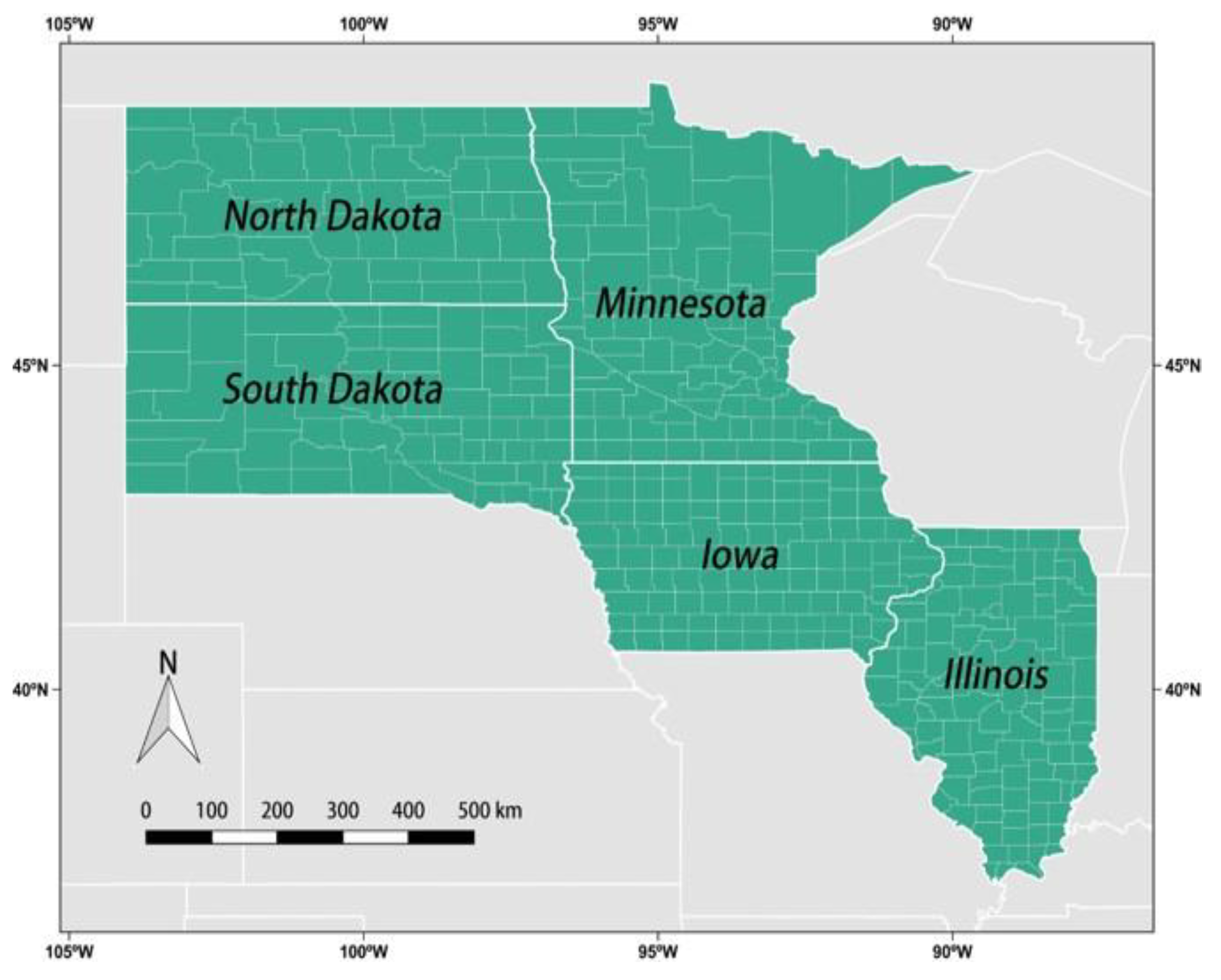
2.1. Study Area
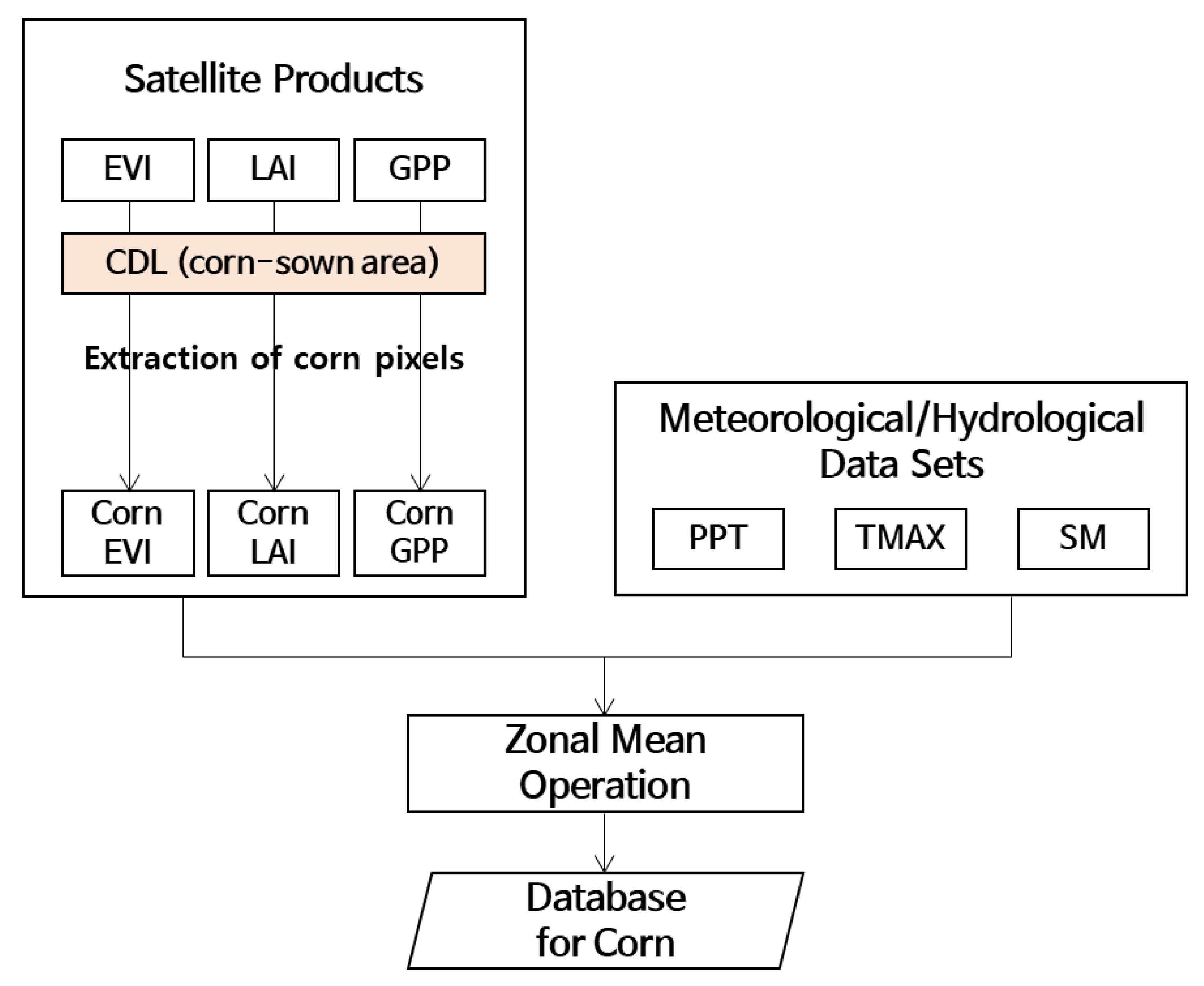
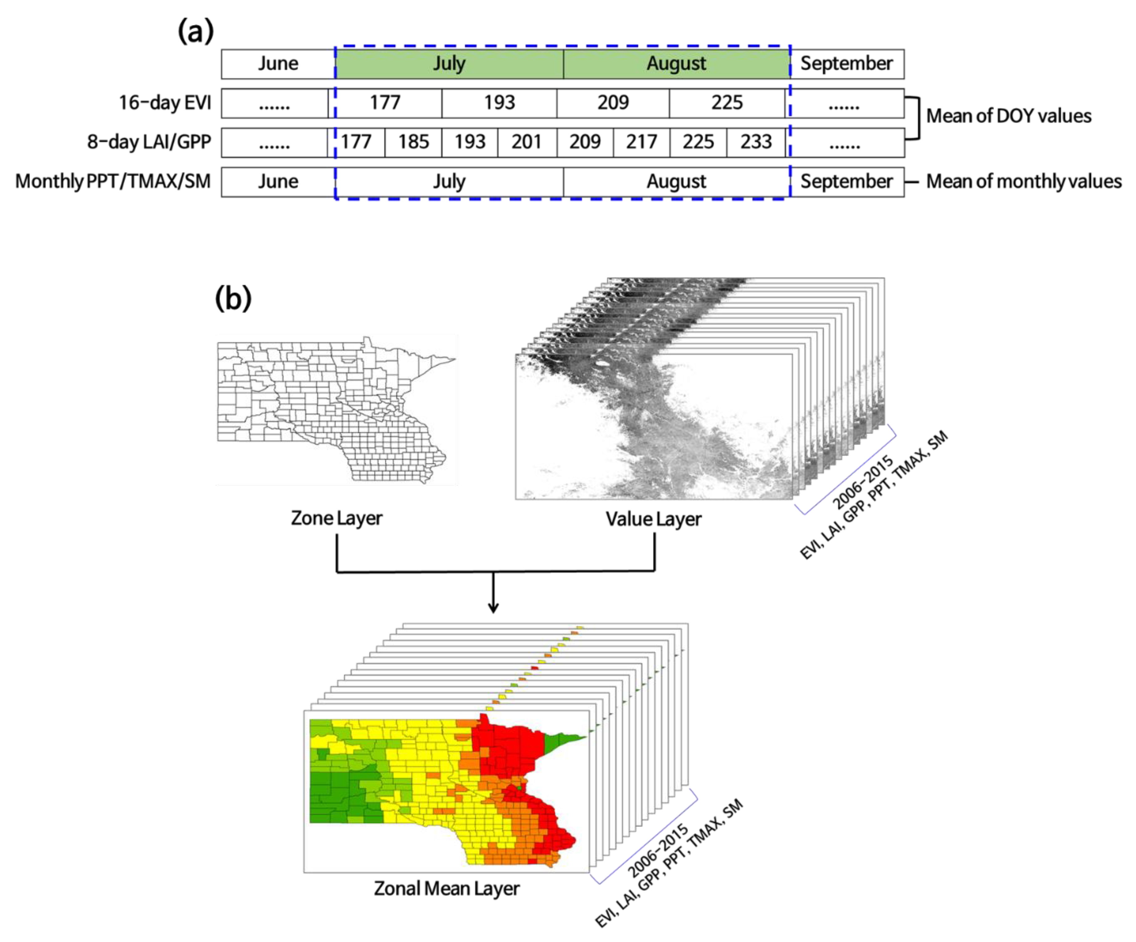
2.2. Data
3. Methods
3.1. Definition of Extreme Weather Events
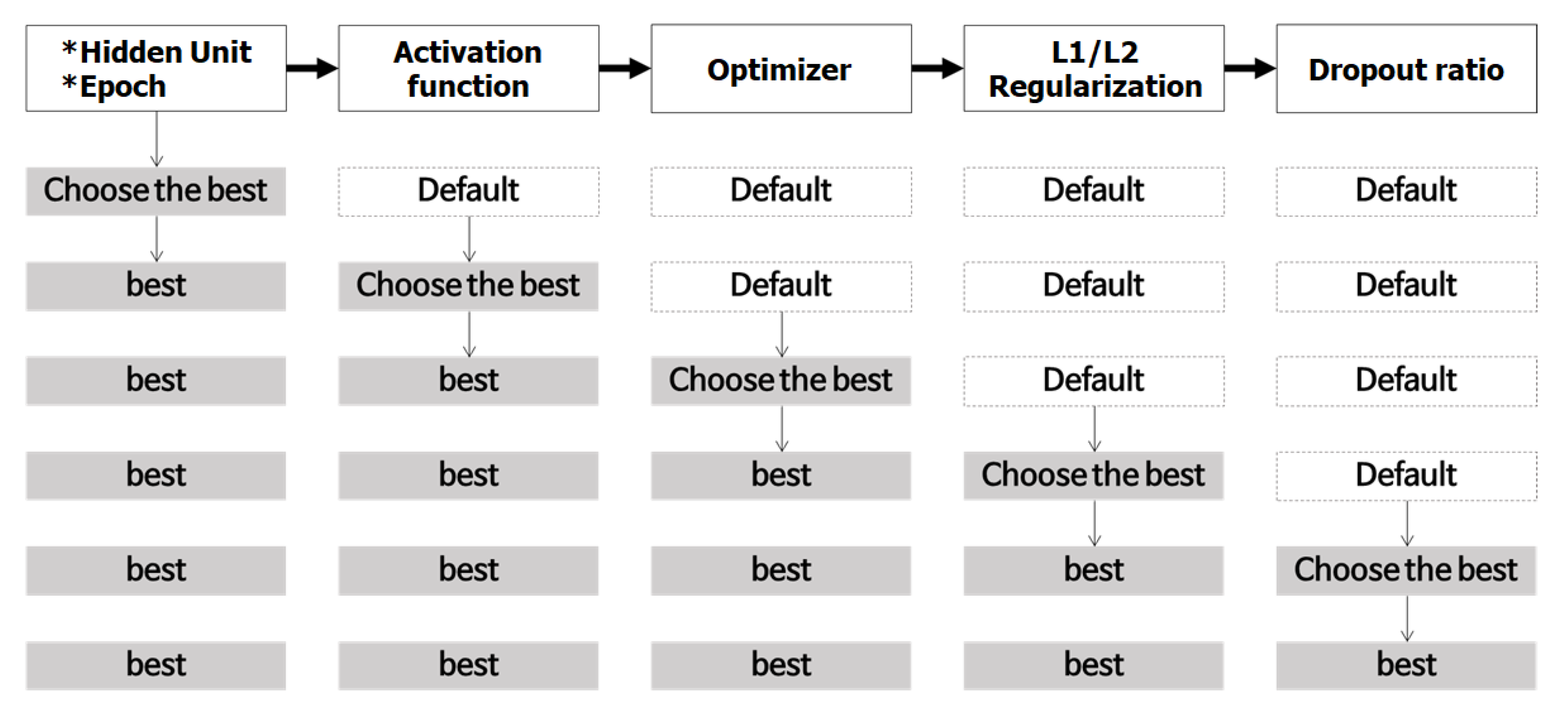
3.2. Artificial Intelligence Models
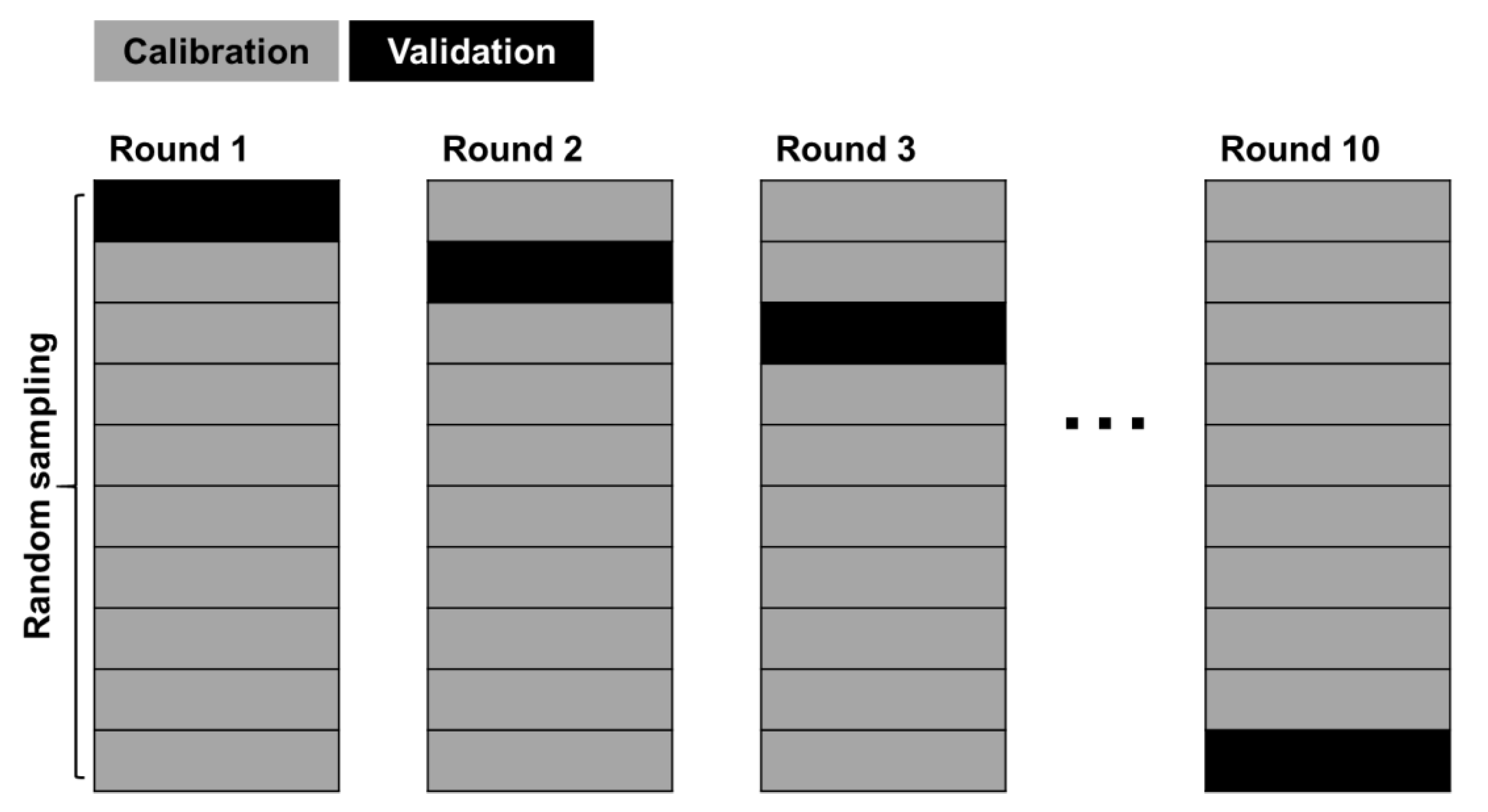
3.3. Training and Validation
4. Results and Discussion
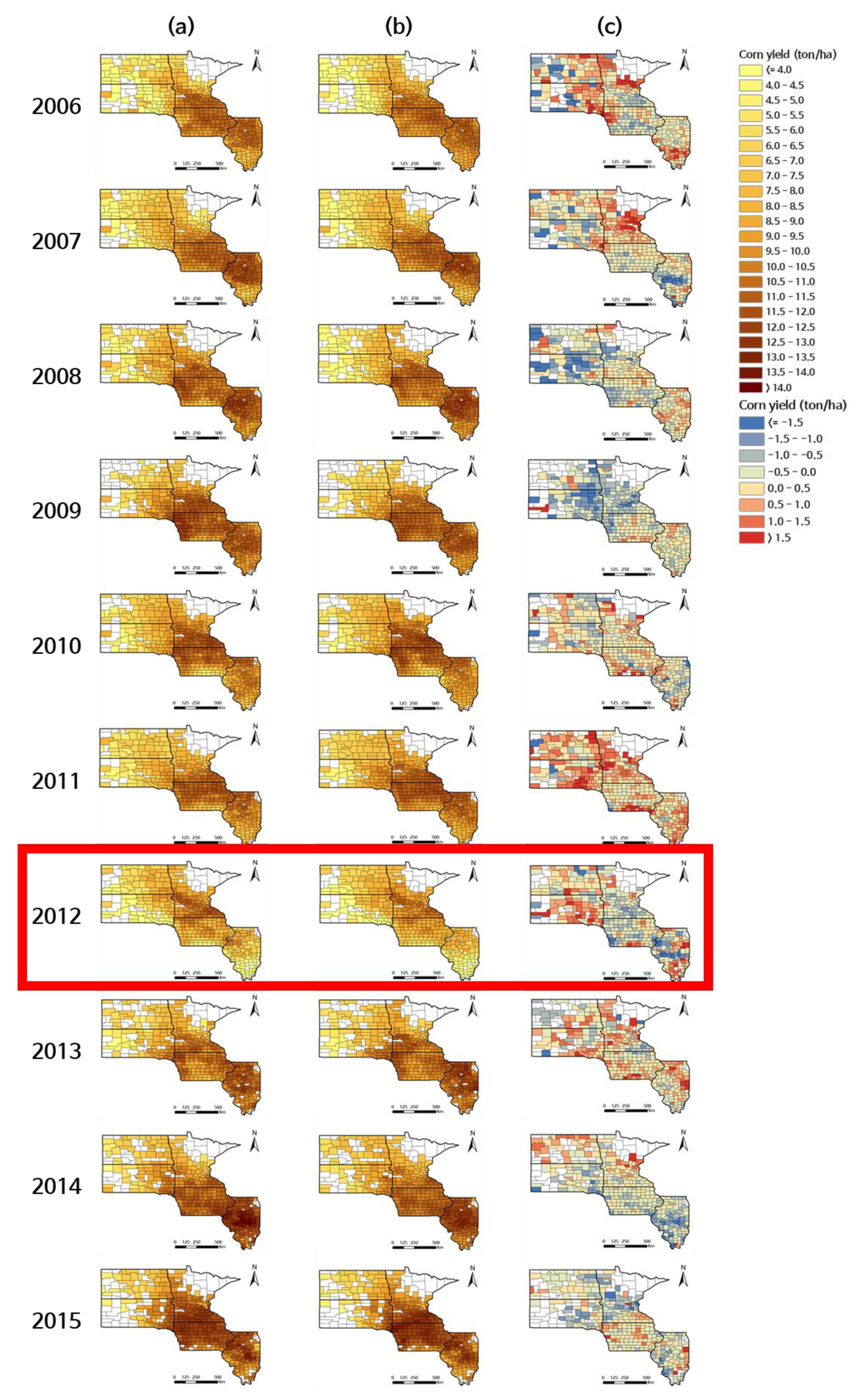
4.1. Experiments under Drought Conditions
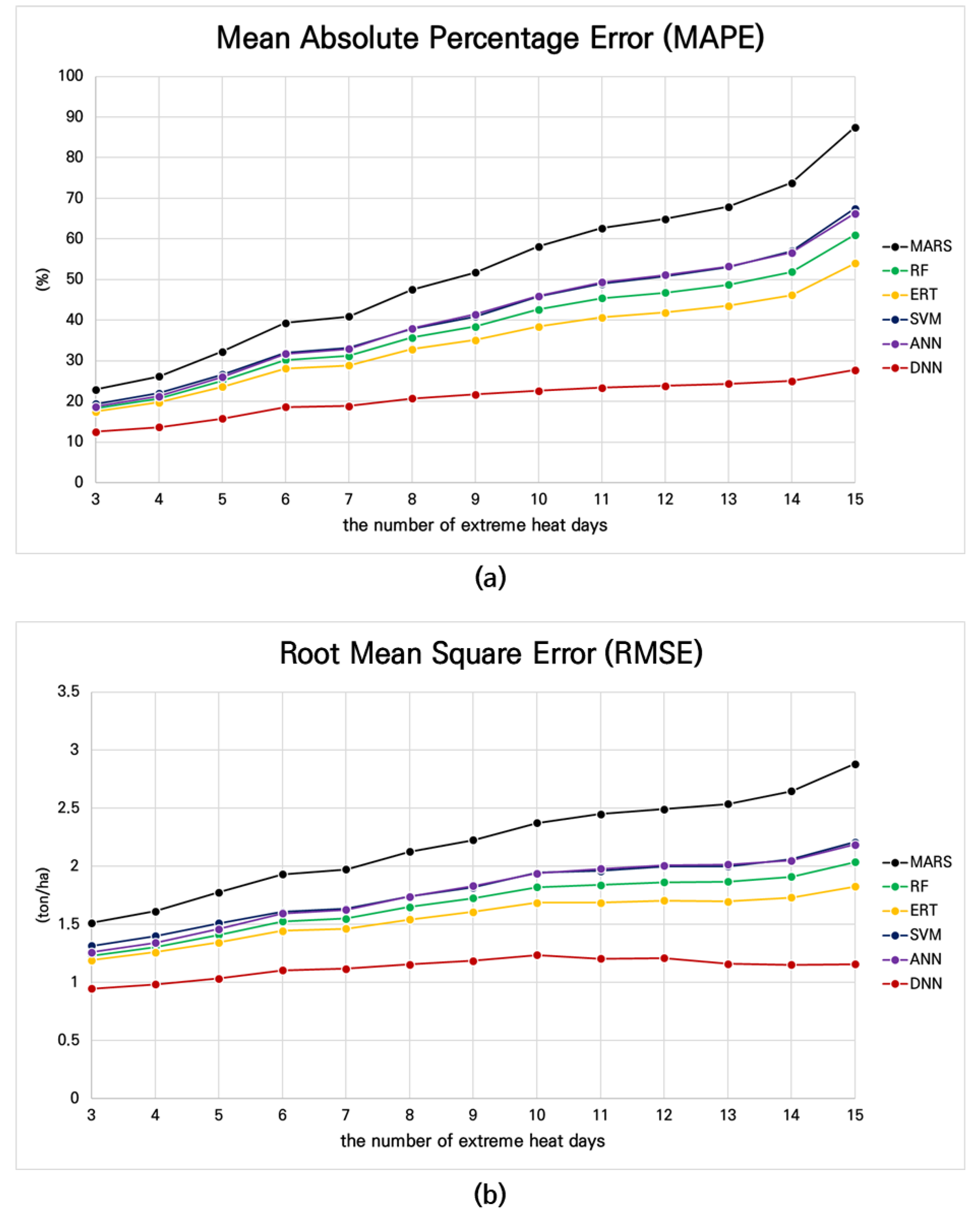
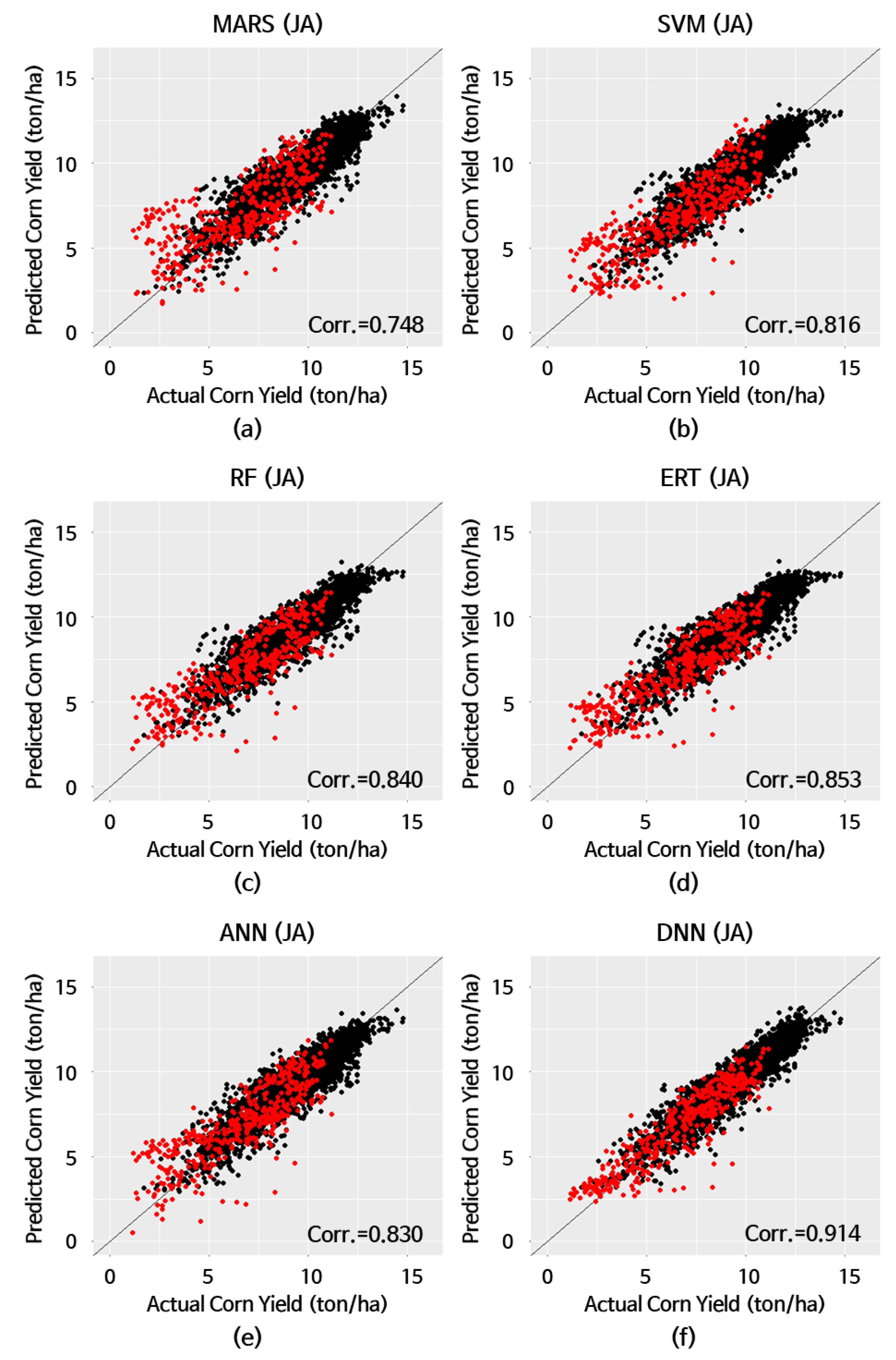
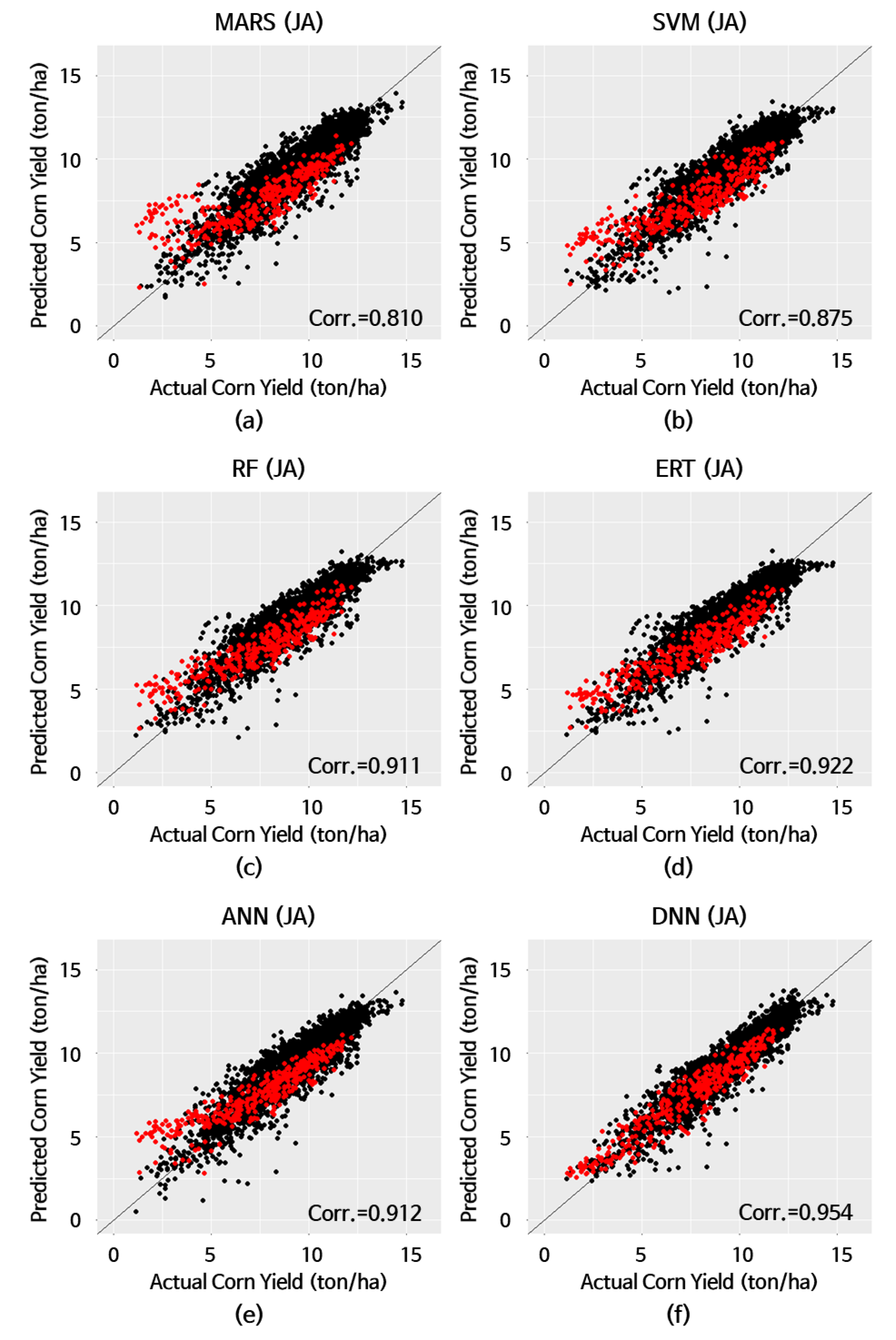
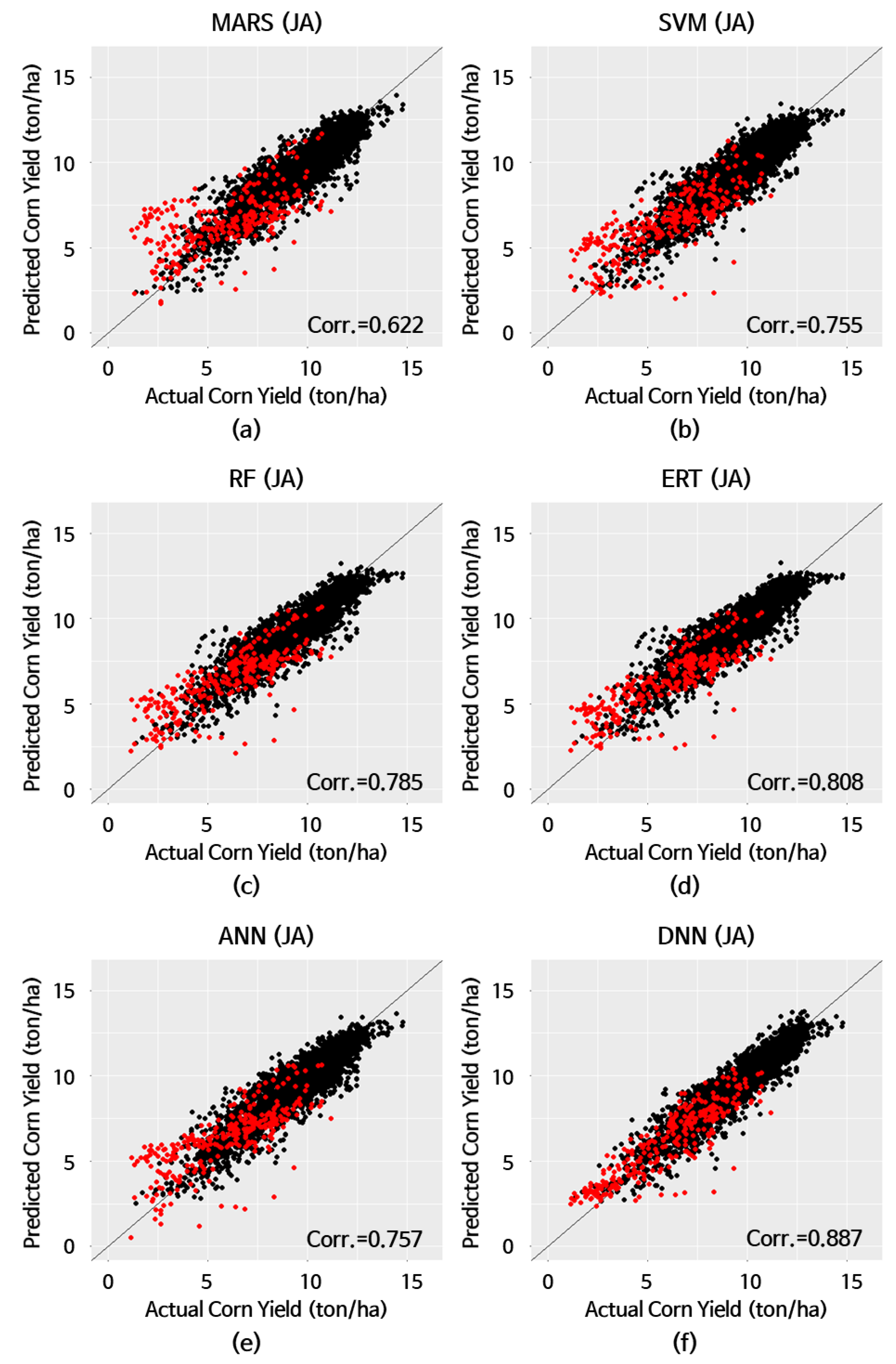
4.2. Experiments under Heatwave Conditions
4.3. Another Type of Blind Test
5. Conclusions
Author Contributions
Funding
Conflicts of Interest
References
- Intergovernmental Panel on Climate Change (IPCC). Climate Change 2014: Impacts, Adaptation and Vulnerability, Part A: Global and Sectoral Aspects, Contribution of Working Group II to the Fifth Assessment Report of the Intergovernmental Panel on Climate Change; Field, C.B., Barros, V.R., Dokken, D.J., Mach, K.J., Mastrandrea, M.D., Bilir, T.E., Chatterjee, M., Ebi, K.L., Estrada, Y.O., Genova, R.C., Eds.; Cambridge University Press: Cambridge, UK; New York, NY, USA, 2014.
- Food and Agriculture Organization of the United Nations (FAO). Available online: http://www.fao.org/news/story/tr/item/44570/icode/en/ (accessed on 1 May 2020).
- National Oceanic and Atmospheric Administration (NOAA) National Climatic Data Center. Available online: http://www.ncdc.noaa.gov/sotc/hazards/2010/7 (accessed on 1 May 2020).
- Lesk, C.; Rowhani, P.; Ramankutty, N. Influence of extreme weather disasters on global crop production. Nature 2016, 529, 84–87. [Google Scholar]
- Teixeira, E.I.; Fischer, G.; Van Velthuizen, H.; Walter, C.; Ewert, F. Global hot-spots of heat stress on agricultural crops due to climate change. Agric. Meteorol. 2013, 170, 206–215. [Google Scholar]
- Iizumi, T.; Shin, Y.; Kim, W.; Kim, M.; Choi, J. Global crop yield forecasting using seasonal climate information from a multi-model ensemble. Clim. Serv. 2018, 11, 13–23. [Google Scholar] [CrossRef]
- Lobell, D.B.; Schlenker, W.; Costa-Roberts, J. Climate trends and global crop production since 1980. Science 2011, 333, 616–620. [Google Scholar] [CrossRef] [Green Version]
- Qian, B.; Zhang, X.; Smith, W.; Grant, B.; Jing, Q.; Cannon, A.J.; Neilsen, D.; McConkey, B.; Li, G.; Bonsal, B.; et al. Climate change impacts on Canadian yields of spring wheat, canola and maize for global warming levels of 1.5 °C, 2.0 °C, 2.5 °C and 3.0 °C. Environ. Res. Lett. 2019, 14, 074005. [Google Scholar]
- Jeong, J.H.; Resop, J.P.; Mueller, N.D.; Fleisher, D.H.; Yun, K.; Butler, E.E.; Timlin, D.J.; Shim, K.-M.; Gerber, J.S.; eddy, V.R.; et al. Random forests for global and regional crop yield predictions. PLoS ONE 2016, 11, e0156571. [Google Scholar]
- Kuwata, K.; Shibasaki, R. Estimating crop yields with deep learning and remotely sensed data. In Proceedings of the 2015 IEEE International Geoscience and Remote Sensing Symposium (IGARSS), Milan, Italy, 26–31 July 2015; pp. 858–861. [Google Scholar]
- Kuwata, K.; Shibasaki, R. Estimating corn yield in the United Sates with MODIS EVI and machine learning methods. ISPRS Ann. Photogramm. Remote Sens. Spat. Inf. Sci. 2016, 3, 131–136. [Google Scholar]
- Kim, N.; Ha, K.-J.; Park, N.-W.; Cho, J.; Hong, S.; Lee, Y.-W. A comparison between major artificial intelligence models for crop yield prediction: Case study of the Midwestern United States, 2006–2015. ISPRS Int. J. Geo Inf. 2019, 8, 240. [Google Scholar]
- Taylor, R.D.; Koo, W.W. Outlook of the U.S. and world corn and soybean industries, 2010–2020. In Agribusiness and Applied Economics Report; North Dakota State University: Fargo, ND, USA, 2011; p. 682. [Google Scholar]
- Food and Agriculture Organization of the United Nations (FAO). FAO Statistical Databases. 2013. Available online: http://faostat.fao.org (accessed on 1 March 2020).
- NASA EARTHDATA Search Home Page. Available online: https://search.earthdata.nasa.gov/ (accessed on 1 March 2020).
- Townshend, J.R.G.; Justice, C.O.; Li, W.; Gurney, C.; McManus, J. Global land cover classification by remote sensing: Present capabilities and future capabilities. Remote Sens. Environ. 1991, 35, 243–255. [Google Scholar]
- Huete, A.R.; Didan, K.; Miura, T.; Rodriguez, E.P.; Gao, X.; Ferreria, L.G. Overview of the radiometric and biophysical performance of the MODIS vegetation indices. Remote Sens. Environ. 2002, 83, 195–213. [Google Scholar] [CrossRef]
- Sellers, P.J. Canopy reflectance, photosynthesis and transpiration. Int. J. Remote Sens. 1985, 6, 1335–1372. [Google Scholar] [CrossRef]
- Lee, S.-J.; Cho, J.; Hong, S.; Ha, K.-J.; Lee, H.; Lee, Y.-W. On the relationships between satellite-based drought index and gross primary production in the North Korean croplands, 2000–2012. Remote Sens. Lett. 2016, 7, 790–799. [Google Scholar] [CrossRef]
- PRISM Climate Group Home Page. Available online: http://www.prism.oregonstate.edu/ (accessed on 1 March 2020).
- GES DISC Home Page. Available online: https://disc.gsfc.nasa.gov/ (accessed on 1 March 2020).
- Rodell, M.; Houser, P.R.; Jambor, U.; Gottschalck, J.; Mitchell, K.; Meng, C.-J.; Arsenault, K.; Cosgrove, B.; Radakovich, J.; Bosilovich, M.; et al. The global land data assimilation system. Bull. Am. Meteorol. Soc. 2004, 85, 381–394. [Google Scholar] [CrossRef] [Green Version]
- De Jeu, R.; Holmes, T.; Dorigo, W.; Wagner, W.; Hahn, S.; Parinussa, R. Evaluation of SMOS soil moisture with other existing satellite products. In Proceedings of the Remote Sensing and Hydrology 2010 Symposium, Jackson Hole, WY, USA, 27–30 September 2010. [Google Scholar]
- NASS USDA Home Page. Available online: https://www.nass.usda.gov/ (accessed on 1 March 2020).
- Boryan, C.; Yang, Z.; Mueller, R.; Craig, M. Monitoring US agriculture: The US department of agriculture, national agricultural statistics service, cropland data layer program. Geocarto Int. 2011, 26, 341–358. [Google Scholar] [CrossRef]
- Becker-Reshef, I.; Vermote, E.; Lindeman, M.; Justice, C. A generalized regression-based model for forecasting winter wheat yields in Kansas and Ukraine using MODIS data. Remote Sens. Environ. 2010, 114, 1312–1323. [Google Scholar] [CrossRef]
- NASS USDA Quick Stats Home Page. Available online: http://quickstats.nass.usda.gov (accessed on 1 March 2020).
- Wilhite, D.A.; Glantz, M.H. Understanding: The drought phenomenon: The role of definitions. Water Int. 1985, 10, 111–120. [Google Scholar] [CrossRef] [Green Version]
- Quiring, S.M.; Papakryiakou, T.N. An evaluation of agricultural drought indices for the Canadian prairies. Agric. For. Meteorol. 2003, 118, 49–62. [Google Scholar] [CrossRef]
- Vicente-Serrano, S.M.; Gouveia, C.; Camarero, J.J.; Beguería, S.; Trigo, R.; López-Moreno, J.I.; Azorín-Molina, C.; Pasho, E.; Lorenzo-Lacruz, J.; Revuelto, J.; et al. Response of Vegetation to Drought Time-Scales across Global Land Biomes. Proc. Natl. Acad. Sci. USA 2013, 110, 52–57. [Google Scholar] [CrossRef] [Green Version]
- Crutchfiled, S.U.S. Drought 2012: Farm and Food Impacts; USDA Economic Research Service: Washington, DC, USA, 2012.
- Global Vegetation Health Products. Available online: https://www.star.nesdis.noaa.gov/smcd/emb/vci/VH/index.php (accessed on 18 May 2020).
- Palmer Drought Severity Index (PDSI). Available online: https://climatedataguide.ucar.edu/climate-data/palmer-drought-severity-index-pdsi (accessed on 18 May 2020).
- Lee, K.; Kang, H.-S.; Cho, C.H. Climate change-induced high temperature stress on global crop production. Korean Geogr. Soc. 2016, 51, 622–649. [Google Scholar]
- Challinor, A.J.; Wheeler, T.R.; Craufurd, P.Q.; Slingo, J.M. Simulation of the impact of high temperature stress on annual crop yields. Agric. Meteorol. 2005, 135, 180–189. [Google Scholar] [CrossRef] [Green Version]
- Hastie, T.; Tibshirani, R.; Friedman, J. The Elements of Statistical Learning: Data Mining, Inference and Prediction, 2nd ed.; Springer: New York, NY, USA, 2009. [Google Scholar]
- Pal, M.; Mather, P.M. An assessment of the effectiveness of decision tree methods for land cover classification. Remote Sens. Environ. 2003, 86, 554–565. [Google Scholar]
- Jensen, J.R.; Im, J.; Hardin, P.; Jense, R.R. Image Classification. In The Sage Handbook of Remote Sensing; Warner, T.A., Nellis, M.D., Foody, G.M., Eds.; SAGE Publications Ltd.: London, UK, 2009; Chapter 19; pp. 269–296. [Google Scholar]
- Duro, D.C.; Franklin, S.E.; Dube, M.G. A comparison of pixel-based and object-based image analysis with selected machine learning algorithms for the classification of agricultural landscapes using SPOT-5 HRG imagery. Remote Sens. Environ. 2012, 118, 259–272. [Google Scholar] [CrossRef]
- Mountrakis, G.; Im, J.; Ogole, C. Support vector machines in remote sensing: A review. ISPRS J. Photogramm. Remote Sens. 2011, 66, 247–259. [Google Scholar] [CrossRef]
- Foody, G.M.; Mathur, A. The use of small training sets containing mixed pixels for accurate hard image classification: Training on mixed spectral responses for classification by SVM. Remote Sens. Environ. 2006, 103, 179–189. [Google Scholar]
- Van der Linder, S.; Hoster, P. The influence of urban structures on impervious surface maps from airborne hyperspectral data. Remote Sens. Environ. 2009, 113, 2298–2305. [Google Scholar] [CrossRef]
- Breiman, L.; Culter, A. Random Forests. 2014. Available online: http://www.stat.berkeley.edu/~breiman/RandomForests/cc_home.htm (accessed on 1 March 2020).
- Breiman, L. Random forests. Mach. Learn. 2001, 45, 5–32. [Google Scholar] [CrossRef] [Green Version]
- Ali, J.; Khan, R.; Ahmad, N.; Maqsood, I. Random forests and decision trees. Int. J. Comput. Sci. Issues 2012, 9, 272–278. [Google Scholar]
- Geurts, P.; Ernst, D.; Wehenkel, L. Extremely randomized trees. Mach. Learn. 2006, 63, 3–42. [Google Scholar]
- Kaul, M.; Hill, R.L.; Walthall, C. Artificial neural networks for corn and soybean yield prediction. Agric. Syst. 2005, 85, 1–18. [Google Scholar]
- Brown, M.E.; Lary, D.J.; Vrieling, A.; Stathakis, D.; Mussan, H. Neural networks as a tool for constructing continuous NDVI time series from AVHRR and MODIS. Int. J. Remote Sens. 2008, 29, 7141–7158. [Google Scholar] [CrossRef] [Green Version]
- Ji, B.; Sun, Y.; Yang, S.; Wan, J. Artificial neural networks for rice yield prediction in mountainous regions. J. Agric. Sci. 2007, 145, 249–261. [Google Scholar] [CrossRef]
- Pham, V.; Bluche, T.; Kernorvant, C.; Louradour, J. Drop-out improves recurrent neural networks for handwriting recognition. In Proceedings of the 2014 14th International Conference on Frontiers in Handwriting Recognition (ICFHR), Crete, Greece, 1–4 September 2014. [Google Scholar]
- Erhan, D.; Bengio, Y.; Courville, A.; Manzagol, P.A.; Vincent, P. Why does unsupervised pre-training help deep learning? J. Mach. Learn. Res. 2010, 11, 625–660. [Google Scholar]
- Classen, M.M.; Shaw, R.H. Water deficit effects on corn. I. Grain components. Agron. J. 1970, 62, 652–655. [Google Scholar] [CrossRef]
- Carlson, R.E. Heat stress, plant-available soil moisture, and corn yields in Iowa: A short- and long-term view. J. Prod. Agric. 2013, 3, 293–297. [Google Scholar]
- Thomas, J.F.; Raper, C.D.; Weeks, W.W. Day and night temperature effects on nitrogen and soluble carbohydrate allocation during early reproductive growth in soybeans. Agron. J. 1981, 73, 577–582. [Google Scholar] [CrossRef]
- Wallace, D.H. Physiological genetics of plant maturity, adaptation, and yield. In Plant Breeding Review; Janick, J., Ed.; John Wiley & Sons, Inc.: Hoboken, NJ, USA, 1985; Volume 3, pp. 21–167. [Google Scholar]


| Data | Spatial Resolution | Temporal Resolution | Source | |
|---|---|---|---|---|
| Cropland | CDL (1) | 56 m (2006–2009) 30 m (2010–2015) | Yearly | USDA (8) |
| Satellite images | EVI (2) | 250 m | 16 days | NASA EOSDIS (9) |
| LAI (3) | 500 m | 8 days | ||
| GPP (4) | ||||
| Meteorological data | PPT (5) | 4 km | Monthly | PRISM (10) Climate Group |
| TMAX (6) | ||||
| Hydrological data | SM (7) | 25 km | Monthly | NASA GES DISC (11) |
| Yield statistics | Corn | County | Yearly | USDA (8) |
| Year | Corn Yield (ton/ha) | PPT (mm/Month) | TMIN (°C) | TMAX (°C) | TMEAN (°C) | VHI (0 to 100) | PDSI (Unitless) |
|---|---|---|---|---|---|---|---|
| 2006 | 8.519 | 85.6 | 17.0 | 29.8 | 23.4 | 45.2 | −0.886 |
| 2007 | 8.871 | 103.5 | 16.6 | 29.1 | 22.8 | 49.0 | 1.083 |
| 2008 | 9.420 | 83.8 | 15.6 | 28.3 | 21.9 | 58.0 | 2.855 |
| 2009 | 10.061 | 105.4 | 14.3 | 26.0 | 20.1 | 68.7 | 2.890 |
| 2010 | 9.167 | 119.5 | 17.4 | 29.3 | 23.3 | 61.1 | 4.953 |
| 2011 | 8.938 | 82.9 | 17.6 | 29.6 | 23.6 | 61.3 | 3.288 |
| 2012 | 7.352 | 52.9 | 16.6 | 30.9 | 23.7 | 32.2 (1) | −3.336 (2) |
| 2013 | 9.489 | 52.1 | 15.7 | 28.0 | 21.9 | 58.5 | −0.207 |
| 2014 | 10.265 | 99.5 | 15.5 | 26.7 | 21.1 | 70.1 | 1.149 |
| 2015 | 10.651 | 112.1 | 15.6 | 27.3 | 21.5 | 65.0 | 1.066 |
| Mean | 9.283 | 89.7 | 16.2 | 28.5 | 22.3 | 56.9 | 1.286 |
| Model | Hyperparameters (Optimized) | Library Used |
|---|---|---|
| MARS (1) | Pruning method: backward | earth library in R |
| SVM (2) | Kernel function: Gaussian radial basis function | e1071 library in R |
| RF (3) | Number of trees: 500 Number of variables used for splitting nodes: n/3 (n is the number of input variables) | randomForest library in R |
| ERT (4) | Number of trees: 500 Number of variables used for splitting nodes: n/3 (n is the number of input variables) | extraTrees library in R |
| ANN (5) | Number of hidden units: 3 | nnet library in R |
| DNN (6) | Hidden units: 300–300 Loss function: Sum of Squared Errors (SSE) Activation function: Rectified Linear Unit (ReLU) Optimizer: Adaptive Gradient (AdaGrad) Dropout ratio: 40% | tensorflow library in Python |
| Model | MBE (1) (ton/ha) | MAE (2) (ton/ha) | RMSE (3) (ton/ha) | MAPE (4) (%) | Corr.(5) |
|---|---|---|---|---|---|
| MARS (6) | 0.168 | 1.153 | 1.643 | 29.2 | 0.810 |
| SVM (7) | 0.019 | 1.123 | 1.423 | 25.0 | 0.875 |
| RF (8) | 0.068 | 1.025 | 1.303 | 23.2 | 0.911 |
| ERT (9) | −0.056 | 1.012 | 1.248 | 21.6 | 0.922 |
| ANN (10) | 0.171 | 0.975 | 1.304 | 23.7 | 0.912 |
| DNN (11) | −0.017 | 0.666 | 0.828 | 12.9 | 0.954 |
| No. of Years for Training | No. of Experiments (1) | MBE (2) (ton/ha) | MAE (3) (ton/ha) | RMSE (4) (ton/ha) | MAPE (5) (%) | Corr.(6) |
|---|---|---|---|---|---|---|
| 3 years | 20 out of 9C3 | 0.070 | 0.920 | 1.154 | 19.0 | 0.919 |
| 5 years | 20 out of 9C5 | −0.091 | 0.915 | 1.153 | 19.1 | 0.926 |
| 7 years | 20 out of 9C7 | 0.007 | 0.874 | 1.090 | 18.2 | 0.931 |
| 9 years | 1 (9C9) | −0.017 | 0.666 | 0.828 | 12.9 | 0.954 |
| Models | MBE (1) (ton/ha) | MAE (2) (ton/ha) | RMSE (3) (ton/ha) | MAPE (4) (%) | Corr.(5) |
|---|---|---|---|---|---|
| Current model (w/ SM (6)) | −0.017 | 0.666 | 0.828 | 12.9 | 0.954 |
| Current model (w/ SM) + VHI (7) | −0.038 | 0.618 | 0.791 | 11.4 | 0.954 |
| Current model (w/ SM) + PDSI (8) | −0.021 | 0.704 | 0.914 | 12.5 | 0.937 |
| Current model (w/ SM) + VHI + PDSI | 0.013 | 0.632 | 0.818 | 11.4 | 0.950 |
| Model | MBE (1) (ton/ha) | MAE (2) (ton/ha) | RMSE (3) (ton/ha) | MAPE (4) (%) | Corr.(5) | |
|---|---|---|---|---|---|---|
| HW≧5 (6) | MARS (8) | 0.490 | 1.352 | 1.776 | 32.3 | 0.748 |
| SVM (9) | 0.328 | 1.180 | 1.510 | 26.6 | 0.816 | |
| RF (10) | 0.326 | 1.104 | 1.411 | 25.1 | 0.840 | |
| ERT (11) | 0.257 | 1.068 | 1.345 | 23.6 | 0.853 | |
| ANN (12) | 0.350 | 1.119 | 1.459 | 26.0 | 0.830 | |
| DNN (13) | 0.108 | 0.781 | 1.033 | 15.8 | 0.914 | |
| HW≧7(7) | MARS (8) SVM (9) | 0.546 0.445 | 1.514 1.278 | 1.974 1.638 | 40.9 33.1 | 0.622 0.755 |
| RF (10) ERT(11) | 0.401 0.307 | 1.220 1.165 | 1.550 1.463 | 31.2 28.9 | 0.785 0.808 | |
| ANN (12) DNN (13) | 0.414 0.101 | 1.263 0.857 | 1.626 1.117 | 32.9 18.9 | 0.757 0.887 |
| Validation Method | MBE (1) (ton/ha) | MAE (2) (ton/ha) | RMSE (3) (ton/ha) | MAPE (4) (%) | Corr.(5) | |
|---|---|---|---|---|---|---|
| Drought | leave-one-year-out | −0.017 | 0.666 | 0.828 | 12.9 | 0.954 |
| 10-fold | −0.001 | 0.694 | 0.934 | 12.6 | 0.934 | |
| HW ≧ 5 (6) | leave-one-year-out | 0.108 | 0.781 | 1.033 | 15.8 | 0.914 |
| 10-fold | 0.019 | 0.780 | 1.079 | 15.9 | 0.906 | |
| HW ≧ 7 (7) | leave-one-year-out | 0.101 | 0.857 | 1.117 | 18.9 | 0.887 |
| 10-fold | 0.083 | 0.863 | 1.179 | 19.0 | 0.875 |
© 2020 by the authors. Licensee MDPI, Basel, Switzerland. This article is an open access article distributed under the terms and conditions of the Creative Commons Attribution (CC BY) license (http://creativecommons.org/licenses/by/4.0/).
Share and Cite
Kim, N.; Na, S.-I.; Park, C.-W.; Huh, M.; Oh, J.; Ha, K.-J.; Cho, J.; Lee, Y.-W. An Artificial Intelligence Approach to Prediction of Corn Yields under Extreme Weather Conditions Using Satellite and Meteorological Data. Appl. Sci. 2020, 10, 3785. https://doi.org/10.3390/app10113785
Kim N, Na S-I, Park C-W, Huh M, Oh J, Ha K-J, Cho J, Lee Y-W. An Artificial Intelligence Approach to Prediction of Corn Yields under Extreme Weather Conditions Using Satellite and Meteorological Data. Applied Sciences. 2020; 10(11):3785. https://doi.org/10.3390/app10113785
Chicago/Turabian StyleKim, Nari, Sang-Il Na, Chan-Won Park, Morang Huh, Jaiho Oh, Kyung-Ja Ha, Jaeil Cho, and Yang-Won Lee. 2020. "An Artificial Intelligence Approach to Prediction of Corn Yields under Extreme Weather Conditions Using Satellite and Meteorological Data" Applied Sciences 10, no. 11: 3785. https://doi.org/10.3390/app10113785
APA StyleKim, N., Na, S.-I., Park, C.-W., Huh, M., Oh, J., Ha, K.-J., Cho, J., & Lee, Y.-W. (2020). An Artificial Intelligence Approach to Prediction of Corn Yields under Extreme Weather Conditions Using Satellite and Meteorological Data. Applied Sciences, 10(11), 3785. https://doi.org/10.3390/app10113785