Evaluating the Performance of Individual and Novel Ensemble of Machine Learning and Statistical Models for Landslide Susceptibility Assessment at Rudraprayag District of Garhwal Himalaya

Abstract

Landslides are known as the world’s most dangerous threat in mountainous regions and pose a critical obstacle for both economic and infrastructural progress. It is, therefore, quite relevant to discuss the pattern of spatial incidence of this phenomenon. The current research manifests a set of individual and ensemble of machine learning and probabilistic approaches like an artificial neural network (ANN), support vector machine (SVM), random forest (RF), logistic regression (LR), and their ensembles such as ANN-RF, ANN-SVM, SVM-RF, SVM-LR, LR-RF, LR-ANN, ANN-LR-RF, ANN-RF-SVM, ANN-SVM-LR, RF-SVM-LR, and ANN-RF-SVM-LR for mapping landslide susceptibility in Rudraprayag district of Garhwal Himalaya, India. A landslide inventory map along with sixteen landslide conditioning factors (LCFs) was used. Randomly partitioned sets of 70%:30% were used to ascertain the goodness of fit and predictive ability of the models. The contribution of LCFs was analyzed using the RF model. The altitude and drainage density were found to be the responsible factors in causing the landslide in the study area according to the RF model. The robustness of models was assessed through three threshold dependent measures, i.e., receiver operating characteristic (ROC), precision and accuracy, and two threshold independent measures, i.e., mean-absolute-error (MAE) and root-mean-square-error (RMSE). Finally, using the compound factor (CF) method, the models were prioritized based on the results of the validation methods to choose best model. Results show that ANN-RF-LR indicated a realistic finding, concentrating only on 17.74% of the study area as highly susceptible to landslide. The ANN-RF-LR ensemble demonstrated the highest goodness of fit and predictive capacity with respective values of 87.83% (area under the success rate curve) and 93.98% (area under prediction rate curve), and the highest robustness correspondingly. These attempts will play a significant role in ensemble modeling, in building reliable and comprehensive models. The proposed ANN-RF-LR ensemble model may be used in the other geographic areas having similar geo-environmental conditions. It may also be used in other types of geo-hazard modeling.

1. Introduction

The landmass movement is the physical process in downhill geomorphic regions, which causes rolls of rubble, regoliths, and large masses of soil in down slope direction under the impact of gravity. It is a predominantly geological event which takes place when the force of the material exceeds the resistance of the shear strength of the soil [1]. Landslides are ranked as the seventh most destructive geohazard among the various natural hazards prevalent around the world in terms of the magnitude of the loss of lives and properties [2]. The occurrence of landslides depends upon the physiographic, hydrological, geological, and geomorphic setups of the study area. Sometimes, the movement of a large landmass in the hilly regions causes a change in topography, drainage pattern, and courses of rivers. The impact of landslides can be attributed to a wide range of phenomenon such as deforestation, habitat loss of human and wild lives, soil loss, disruption of roads and constructions, and flooding in specific cases [3,4]. In the mountainous landscape, landslides occur frequently, triggered by a heavy rainstorm along with interactions among the various environmental causative factors. According to Raman and Punia [5], around 0.49 million sq.km land of India is under the threat of landslide hazard, which is about 15% of the land area of the country. In Indian sub-continent, landmass movement and failure of slope are mostly activated by a heavy precipitation during monsoon, however in the Himalayan belt, the occurrence of landfalls are pretty normal due to seismic activities viz. the Uttarakhand earthquake in 2017, the Chamoli earthquake in 1999, and the Sikkim earthquake in 2011 [6,7,8,9]. Wadhawan [10] mentioned that the mountainous region of Konkan and the Nilgiri ranges in the south and south-western India and the Western Ghats are severely vulnerable to landslides and mass movements. Other than seismic tremors and rainstorm, human interventions and unplanned encroachment, i.e., construction of roads, civil structures etc., disturb the resistance of landmass and accelerate the rate of landslide occurrence.

Therefore, it is important to know the spatial relationship between the geo-environmental factors and landslide events for quantitative evaluation of landslide susceptibility (LSS). The reliability of analysis and modelling is determined by the quality and availability of input data and methodology employed. Assembling landslide data in mountainous regions is a very challenging task, mostly owing to poor accessibility. Obtaining data through field inspection techniques can be time intensive and costly, and application of remotely sensed data in this regard is fruitful. The literatures suggested that landslide susceptibility zonation has been performed previously using various bivariate and multivariate statistical techniques, such as frequency ratio [11,12], evidential belief function [13,14], statistical index model [15], logistic regression [12,16], weight-of-evidence [15,17], etc. These studies have shown a good accuracy of these techniques in predicting LSS spatially. However, with the advancement of the machine learning-based modelling, LSS has come out as a greater efficient and effective approach in recent decades. There are various studies that used machine learning and artificial intelligence models in performing landslide susceptibility (LSS) assessment such as random forest [18,19], boosted regression tree [12], naïve bayes [20], decision tree [21], neuro-fuzzy [14], artificial neural network [22], support vector machine [20], and many others.

However, one of the major weaknesses of statistical models lies in the fact that some assumptions should be defined before conducting any analysis, and therefore a spatial relationship between causative factors is widely neglected [23]. In contrast, while dealing with the machine learning models, the advantages are they do not need statistical assumptions before analysis and they can deal with data of various types, i.e., categorical and continuous [13]. In this regard, the ensemble models can resolve nonlinear difficulties and complexities [24]. In recent decades, numerous studies were conducted using the ensemble model approach which has shown greater effectiveness in the spatial assessment of various environmental hazards viz. gully erosion susceptibility assessment [25,26], groundwater contamination risk assessment [27], groundwater potential mapping [28], flood risk assessment [29], and landslide vulnerability assessment [30,31].

The main purpose of the predictive models is to recognize the LSS extents depending upon the nature of spatial relationship between causative factors and previous landslides. In this work, we used landslide causative factors using remote sensing data and applied several machine learning models to produce landslide susceptibility maps (LSMs) of Rudraprayag district in Uttarakhand. Subsequently, LSMs were ensemble to attain better accuracy that can be achieved from a single model. The ensemble of the models in the present analysis was implemented in four-stages, whereby in the first stage, individual models were calibrated and then a two-model combination approach was performed, i.e., artificial neural network-random forest (ANN-RF), ANN-support vector machine (ANN-SVM), SVM-RF, SVM-logistic regression (SVM-LR), LR-RF, and LR-ANN. In the second stage, LSS model calibration was performed compiling three model ensemble approaches, i.e., ANN-LR-RF, ANN-RF-SVM, ANN-SVM-LR, RF-SVM-LR. Finally, all four models were combined.

2. Study Area

The Rudraprayag district is located in a highly elevated (2936 feet or 895 m) part of the Garhwal Himalaya in the state of Uttarakhand, India (Figure 1). This downhill district covers an area of 2439 sq. km and geographically extended between 78°49ʹ E and 79°21ʹ2ʹʹ E and from 30°12ʹ N to 30°48ʹ N. According to Hindu mythology, the name of the district comes from the terminology “Rudra” which means “god of wind or storm” in Hindu religion. Because of the unique physiographic set-up of this Himalayan region, the Rudraprayag district is frequently affected by landslides in the past few decades causing deaths and economic losses [32]. The hilly parts of this district are intensely deepened by the major river Alaknanada. Relative relief per unit area is very high (500–3000 m) and the district is categorised under steep-sloped topography. Soil formation is very weak and the layer depth ranges between 0 and 10 m. The geological formation of this area is characterised by Guinness and Dalling sequence, Siwalik rock, Gondwana Park rock and Pleistocene rises. The area lies within the sub-tropical humid region where the highest temperature (25 to 37 °C) prevail in May to July and lowest temperature (2 to 16 °C) recorded between November to February. The average annual precipitation is about 405.17 cm of which 75% to 80% occurs in monsoon (between June and September) when numerous landslides take place (Indian Meteorological Department [33]. Because of its location in a seismic-tectonic disturbance zone and due to anthropogenic interventions (often found along the National Highway 109 and 58 of India), landslides have become a frequent phenomenon in this region. Such topographic, climatic, and anthropogenic frameworks are intensifying the need for the identification of potential areas of landslides in the Rudraprayag district.

3. Materials Used

Topographical map of the study area (sheet no. 78B/5) in 1: 50,000 scale was collected from the Survey of India (SOI), Kolkata which was visually compiled with Google Earth (GE) images from 2017 to 2019 for updating the river map, settlement, and road map. Land use/land covers categories were classified using Sentinel-2 satellite imagery of 10 × 10 m resolution downloaded from the US Geological Survey Earthexplorer [34] which was crosschecked using Cohen’s Kappa coefficient through field truth, GE imagery. The Geological Survey of India provided a detailed lithological map in 1:250,000 scale, which was resampled to match to scale with other thematic layers. To map the seismically disturbed zones, an earthquake zoning map was downloaded and extracted from National Center for Seismology, under the Ministry of Earth Sciences, India in 30 m × 30 m resolution. The lineament was extracted in 1:50,000 scale from the web platform of ISRO (Indian Space Research Organization) that is Bhuvan [35]. Slope, aspect, topographical wetness index (TWI), and stream power index (SPI), were extracted from advanced land observation satellite (ALOS) phased array type L-band synthetic aperture radar (PALSAR) derived digital elevation model (DEM) of 12.5 × 12.5 m resolution downloaded from the Alaska Satellite Facility. Spatial variation of soil depth and texture at 1:50,000 scale was gathered from NBSSLUP Regional Centre, Kolkata and classified based on the texture classification method of U.S. Department of Agriculture (USDA). The rainfall data was collected from the Indian Meteorological Department (

Table 1. Landslide conditioning factors (LCFs), detailed of data used and their respective sources.

LCFS	Data Used	Scale	Sources	Method and Formula	References
Altitude	PALSAR DEM	12.5 m × 12. 5 m	Alaska Satellite	12.5 m × 12. 5 m digital elevation model	[42]
Slope				$\mathrm{Tan}\theta =\frac{N\times i}{636.6}$ N = No. of Contour Cutting; I = Contour Interval	[43]
aspect				$Aspect=57.29578\times a\tan 2(\left[dz/dy\right],-\left[dz/dx\right])$ where, $dz/dx=((c+2f+i)-(a+2d+g))/8$ $dz/dy=((g+2h+i)-(a+2b+c))/8$ Here, a to i indicates the cell value of 3 × 3 window.	[44]
Curvature				$s=\frac{-Z1+Z3+Z7-Z9}{4\times {\Delta }_s^2}$ where Z1–Z9 are altitude values in 3 × 3 cellular networks and ${\Delta }_S$ denotes the cell size.	[45]
SPI				$SPI=As\times \tan (slope)$ where ‘As’ is the specific catchment area in meters.	[46]
Rainfall (cm)	Indian meteorological department	-	https://mausam.imd.gov.in/	Kriging Interpolation method	[47]
Drainage density (sq. km)	Open series toposheets	1:50,000	Survey of India	$DD=\frac{{{\displaystyle \sum }}_1^{n}L}{A}$ where “L” is stream length and “A” is the study area.	[47]
TWI	PALSAR DEM	12.5 m × 12. 5 m	Alaska Satellite	$TWI=\ln \left(\frac{As}{\tan \left(slope\right)}\right)$ where ‘As’ is the specific catchment area in meter and slope in degrees.	[48]
Soil type	Reference district soil map	1:50,000	National Bureau of Soil Survey and Land Use Planning	Digitization process	[49]
Soil depth (m)	Reference district soil map	1:50,000	National Bureau of Soil Survey and Land Use Planning	Digitization process	[49]
Geology	Reference geological map	1:250,000	Geological Survey of India	Digitization process	[49]
Distance to lineaments	Lineaments	1: 50,000	http://bhuvan.nrsc.gov.in	Euclidean distance buffering	[49]
Seismic zones	Last 200 years point data of earthquake	30 m × 30 m	National Centre for Seismology, New Delhi, India	Gridding and interpolation (inverse distance weight method)	[50]
Road Density	Open series toposheets	1:50,000	SOI	$RD=\frac{{{\displaystyle \sum }}_1^{n}Lr}{A}$ where “Lr” is road length and “A” is the study area.	[49]
NDVI	Sentinel-2	10 m × 10 m	https://earthexplorer.usgs.gov.	$NDVI=\frac{NIR-red}{NIR+red}$ where, NIR is near infrared band and IR is the infrared band.	[51]
LU/LC				Supervised classification (Maximum likelihood)	[10]

). However, the spatial resolution of these factors are not same. For producing the landslide susceptibility map, the resolution of the ALOS PALSAR DEM (12.5 m × 12.5 m) was considered as the base resolution and all the causative factors were resembled into 12.5 × 12.5 m resolution.

4. Methodology

This study involved several steps and processes for creating landslide susceptibility (LSS) maps including (Figure 2):

(i)

A total of 223 landslide locations were identified using the high-resolution Google earth images and afterward these locations were verified through field investigation with a global positioning system (GPS) which was conducted during April 2018 and September 2019. The same number of non landslide points as landslide locations were taken randomly for training the models. The 16 environmental factors were considered for modeling (Table 1).

(ii)

Relief-F technique was used to judge the effectiveness of the landslide conditioning factors (LCFs) for LSS mapping.

(iii)

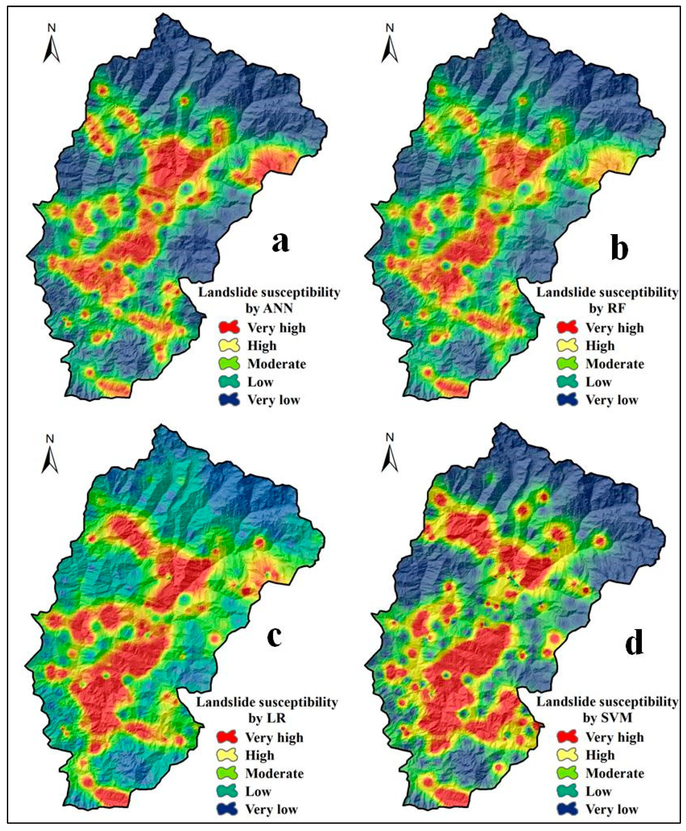
LSS maps first were prepared using ANN, SVM, LR, and RF models. The ensemble models were prepared combining the two, three and four models subsequently.

(iv)

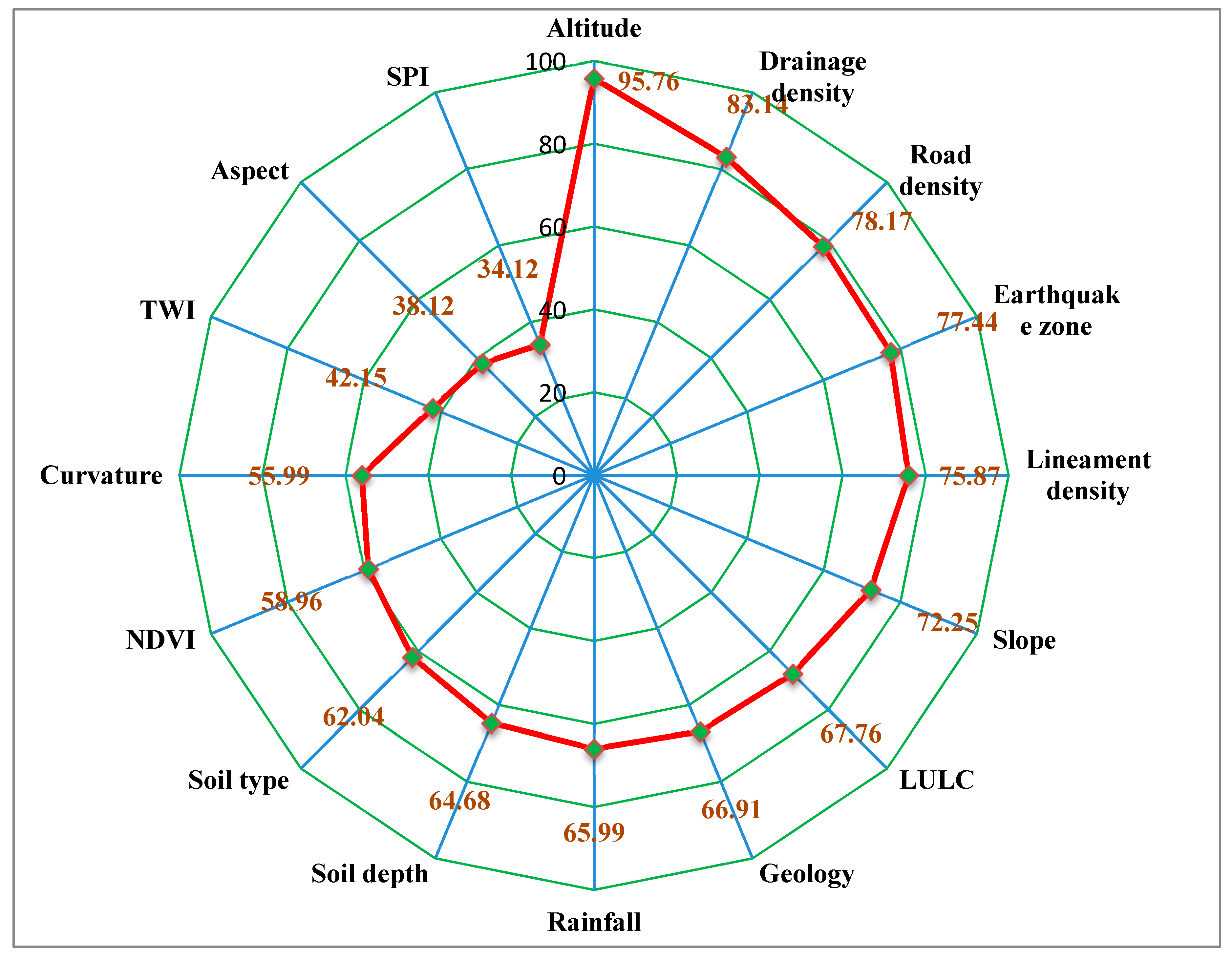
The contribution of the LCFs was assessed using the random forest (RF) model,

(v)

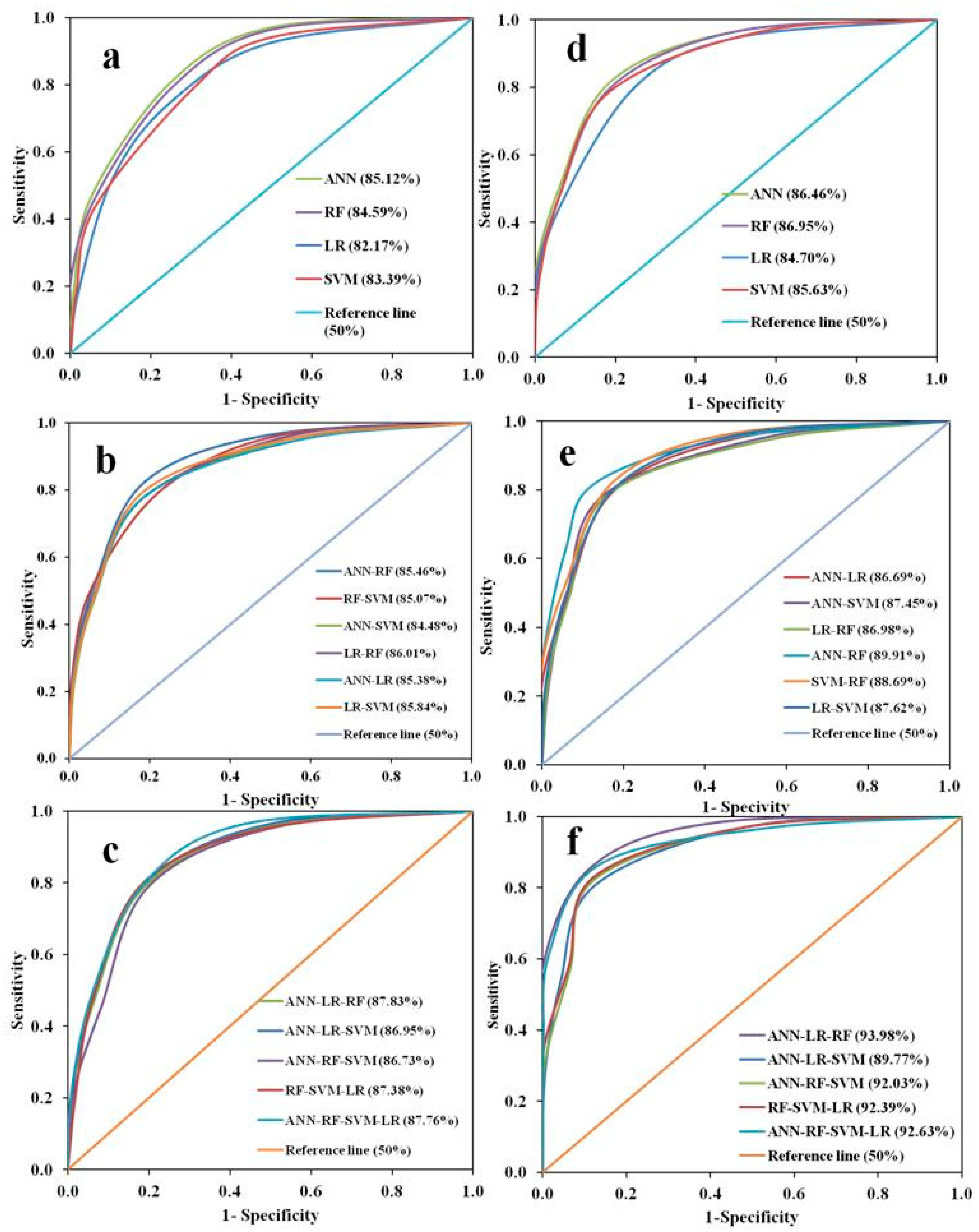
The LSS model’s performances were evaluated through the area under receiver operating characteristic curve (AUCROC), precision, accuracy, mean-absolute-error (MAE), and root-mean-square-error (RMSE).

(vi)

Finally, compound factor (CF) method was used to choose the best model.

4.1. Generation of Landslide Inventory (GLI)

Generation of Landslide Inventory (GLI) is the set of previous and present locations of landslides and is the prerequisite for modeling the landslide susceptibility (LSS). LSS modeling can be assessed through understanding the connections between GLI and landslide causative factors [36]. GLI data set can be prepared through compiling various data sources considering field investigation, past landslide records and evaluation of the Google Earth imageries [37]. In this research, the GLI was prepared by compiling a total of 223 landslide locations recorded in between April 2018 and September 2019 through several field campaigns (Figure 3) using GPS and secondary historical record (record of National Disaster Management Authority, Uttarakhand). Among these inventory, over 40% landslides are translational slides. According to the Uttarakhand National Disaster Management Authority, huge landslides have occurred because of cloudburst rainfall that occurred in July 2019. For training the models, we have selected same amount of non-landslide points randomly over the study area. These historical landslides were then spatially mapped in a 12.5 × 12.5 m resolution, dividing randomly into two sub-set viz. training sub-set, which is comprised of 70% (156 nos.) of GLI and validation or testing sub-set, which includes remaining 30% (67 nos.). The separation of the whole GLI was performed using the extension titled “Geostatistical Analyst” in ArcGIS version of 10.3.1. Training sub-set was used for simulation of the models to generate LSMs and validation sub-set was applied to assess the models’ performances (Figure 1). Landslides mainly occurred in this study area due to rainfall and earthquakes. Rate of landslide has increased with the anthropogenic activities as well. Among the recorded landslides, smallest and largest was 21.73 sq. m and 633.78 sq. m, respectively, while the mean extent was 272.41 sq. m.

4.2. Relief-F Method

Research relief-F is an effective method for the selection of the relevant parameters. Kononenko (1994) [38] suggested various relief models. Investigational outcomes have displayed that Relief-F attains greater performance than the original Relief [39]. It synthesizes the factor weights following their relevance with the goal. Suppose ‘P’ is a randomly selected sample. Then, ‘RWi’ (Relief-F weight) of i-th item can be assessed following Equation (1). One random point can estimate its two nearest neighbors point (one is its same class; other is from diverse class).

$$\begin{array}{c}RWi\leftarrow Wi+\left|P^i-N{H}^i\right|-\left|P^i-N{M}^i\right|\\ \left[\mathrm{here}, \mathrm{NH}=\mathrm{nearest} \mathrm{hit} \mathrm{and} \mathrm{NM}=\mathrm{nearest} \mathrm{miss}\right]\end{array}$$

(1)

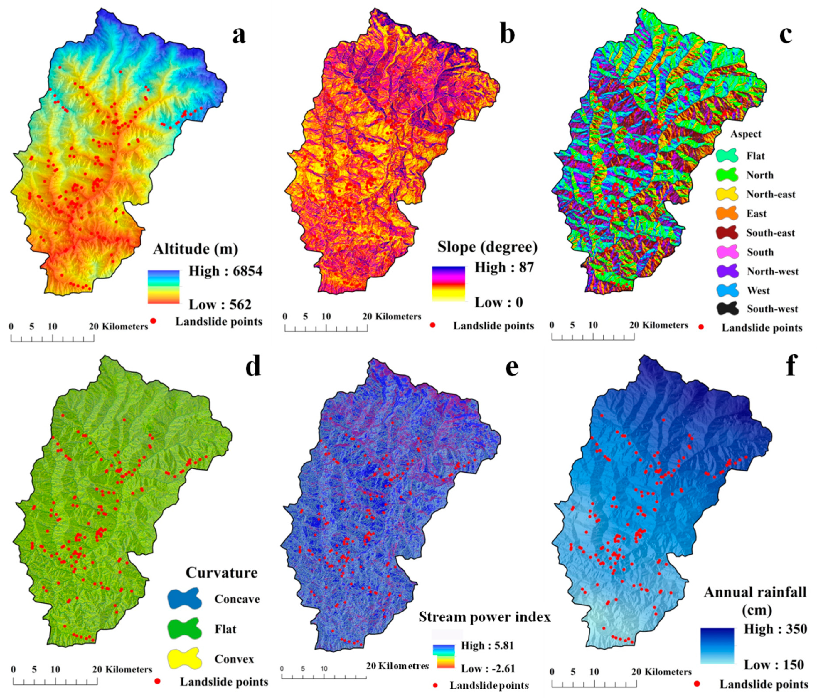
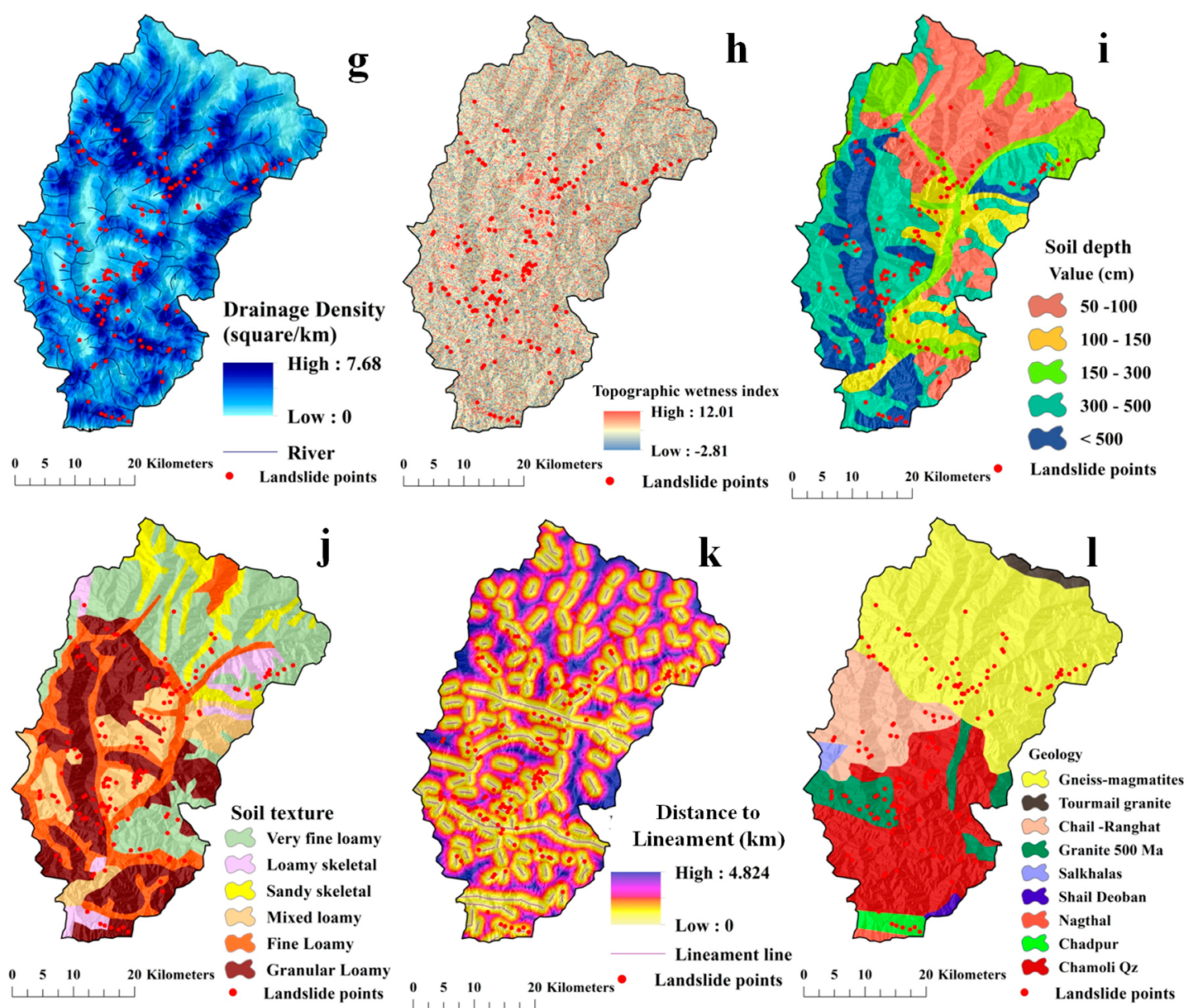
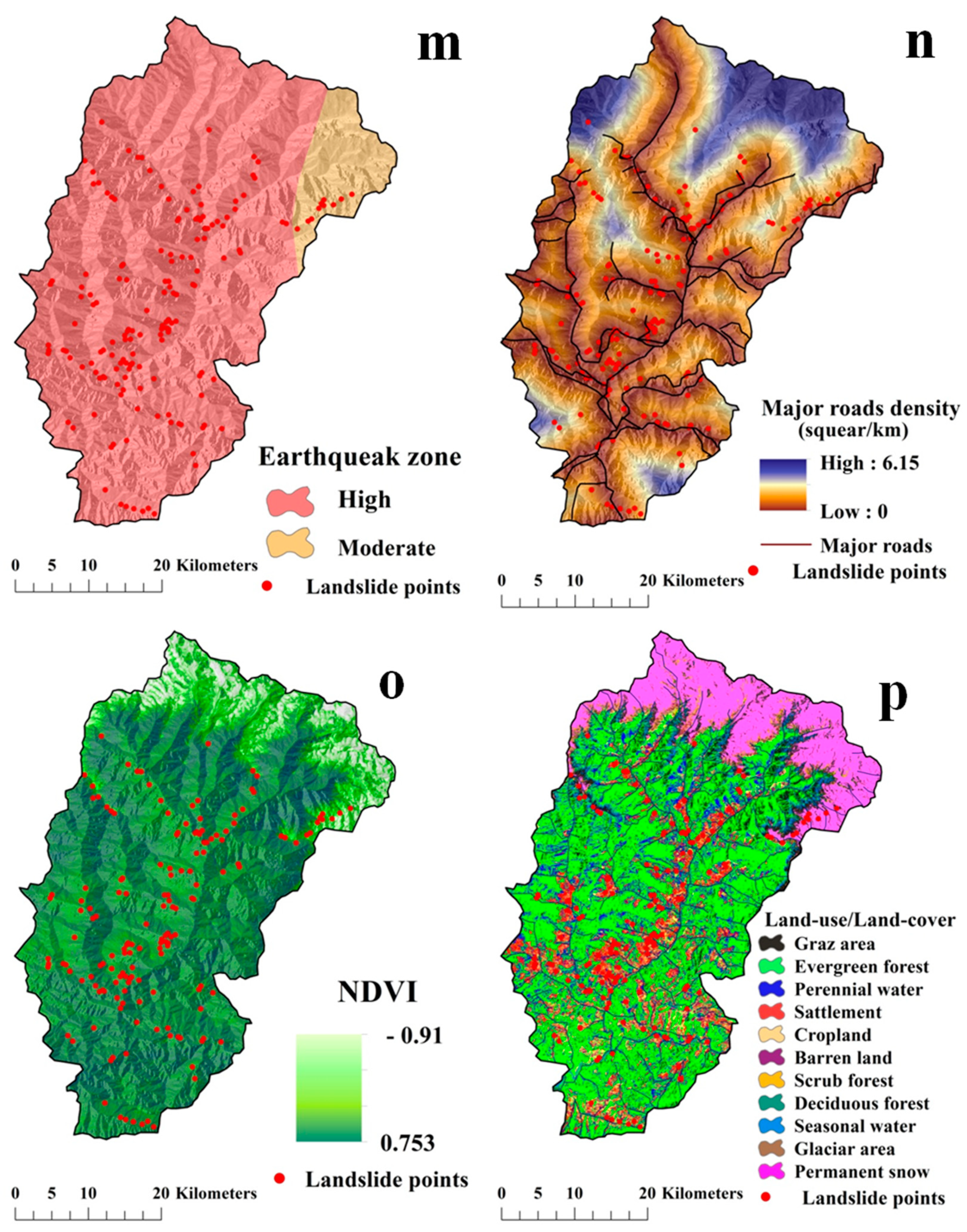
4.3. Preparation of the Landslide Causative Factors (LCFs)

Selection of the causative factors in an analysis is very challenging as it has no determined norms. Similar hydrological, topographical, and environmental variables are not appropriate for modeling and may be varied according to the geographic setting of the regions. In this research, the LCFs were chosen based on the existing literature [10,40,41] and applying the one factor selection method, i.e., Relief-F. For this study, sixteen LCFs were selected for landslide susceptibility mapping. Among the selected factors, rainfall and earthquake zone are landslide triggering factors and the rest are landslide causative factors. The details of the LCFs are given in Table 1.

Topographic LCFs were extracted from a PALSAR DEM with the resolution of 12.5 × 12.5 m using ‘surface’ tool in ArcGIS 10.3.1 software. These LCFs are altitude, slope gradient, slope aspect, curvature and stream power index. Higher altitude areas, especially downhill segments of hilly regions, are favourable for landslides (LS) and the study area has a range of 500 ft. to 2936 ft. elevation (Figure 4a). Slope gradient (Figure 4b) is the result of a combination of factors, i.e., drainage intensity, vegetation, run-off, and geologic. Thus, it was selected as one of the key LCFs in studying landslide susceptibility. The slope angle in the Rudraprayag district varies from 0 to 87° indicating gentle to very-steep gradient. A very steep slope intensifies the potentiality of a landslide (LS) event [40,41]. Duration and magnitude of sunray over the surface is not similar in all facets of slope, which in terms endures varying rate of physical weathering, vegetation growth and soil moisture thereby producing different potential segments for LS hazard. Therefore, slope aspect (Figure 4c) is a vital LCF, particularly in the regions of higher elevation. In the case of curvature (Figure 4d), a rise of curvature value denounces the landslide probability. SPI (Figure 4e) in the process of landmass movement indicates the power of erosion by water which stimulates energy to disintegrate and transport the surface elements.

Hydrological LCFs selected for this study are rainfall, drainage density and topographical wetness index (TWI). For spatial mapping of the rainfall distribution, the precipitation data from 1901 to 2019 (119 years) was considered. The average rainfall map of the study area was prepared using the Kriging method based on the data collected from different stations. Rainfall (Figure 4f) is a widely used LCF in LSS mapping as it triggers the processes like soil slip, debris fall by declining the stability, integration and compaction of the surface forming materials. Towards the north and north-eastern part of the district, amount of average annual rainfall gradually increases from 150 cm to 300 cm. The arrangement of the drainage is the outcome of long-term interactions among geology, topography, climate and lithology. Generally, high intensity of drainages epitomizes low infiltration and prompt run-off and vice versa [52,53]. A large share of the inventory landslides was found along the high drainage density regions (Figure 4g). TWI (Figure 4h) is controlled by topographic factors and the index values represent the tendency of flow accumulation at a specific point and ability of the gravitational forces to flow the water downward in a slope segment [54].

Soil related LCFs in this research are soil texture and soil depth. Six categories of soil texture (Figure 4j) were mapped i.e., coarse loamy, fine loamy mixed loamy, loamy skeletal, loamy sandy, and loamy. Loamy skeletal to the gravelly loamy texture of soil has more erosion susceptibility as it is found in the regions of higher relative relief and drainage density. Higher soil depth with higher elevation in the slope segment designates a higher possibility of the LS hazard (Figure 4i).

Geological factors of the present study are distance to lineaments, geology and earthquake zonation. Areas near to the fault lines are geologically high unstable compared to the distant locations. The lineaments were derived from analyzing satellite images using environment for visualizing images (ENVI) and PCI Geomatica software and from Bhuvan web platform of ISRO. Distances were categorized into five classes (Figure 4k) by applying Jenk’s natural breaks classification scheme. The geological distinctions of this district are Chamoli Quartzite, Tourmaline Granite, Chandpur, Nagthat, Tourmaline Granite, Gneiss-Magmata, Granite 500 Ma, Chail-Ramgarh-Amri, and Shalkhalas-Jutogh (Figure 4l). Numerous past landslide events had occurred in Gneiss-Magmata and Chamoli Quartzite category regions. Occurrence of landslides is also influenced by the earthquake events, seismic disturbances, mountain slope direction and dip direction near the faults. Therefore, the earthquake zonation of the district was included as an LCF in this research. The zones were categorised according to MSK intensity scale (Medvedev–Sponheuer–Karnik scale) in Figure 4m. This scale (

Table 2. Earthquake zonation based on Medvedev–Sponheuer–Karnik (MSK) scale.

Earthquake Zone	MSK Scale	Characteristics
Zone-4	VII. Very strong	Most dwellers are frightened and try to escape outside. Low to medium landmass moved downward.
	VIII. Damaging	Formation of wave on loose surface. Wider cracks and breaches introduce the breakdown of ice.
	IX. Distractive	Disruption of underground pipes. Surface fracturing, large size landfalls.
Zone-5	X. Devastating	Massive landslide may stimulate flooding at surrounding areas and create new bodies of water.
	XI. Catastrophic	Most of the houses/settlements and civil structures are crumbled. Widespread and huge landfall occurs.
	XII. Very catastrophic	Extreme demolition of underground and above-surface infrastructure and households. Landscape transformation, drainage or channel shifting happens.

) helps in evaluating the gravity of the seismic event based on the effect on the district.

Human related factor i.e., road density was considered for the landslide susceptibility mapping. Construction of roadways on the steep slopes removes the support of above landmasses. Removal of the landmass across the slope segment interrupts the stability along the gradient resulting in topographic failure event. Therefore, road density is a vital factor in landslide susceptibility mapping. The landslide inventories showed a tendency of taking place alongside the roadways (Figure 4n).

Environmental LCFs considered in this study are Normalized Difference Vegetation Index (NDVI) and Land Use/Land Cover (LU/LC). NDVI (Figure 4o) is considered as it is the reflection of diverse character of soil properties i.e., moisture, structural composition, climatic event and vegetation types, which are allied with landmass removal processes [51]. Various LU/LC categories exhibit different role in LS hazard in the downhill such as agriculture area and settlement have a positive relation with the landslide (Figure 4p). The district was classified into several broad LU/LCs which are evergreen forest (47.31%), deciduous forest (8.53%), settlement (1.50%), cropland (5.68%), grazing area (6.53%), barren rocky land (8.76%), perennial water bodies (2.05%), glacier region (1.05%), seasonal water body (0.79%), and permanent snow region (15.27%).

4.4. Methods of Landslide Modeling

4.4.1. RF Model

RF was introduced by Breiman [55] and is an extended form of the model CART (Classification and Regression Tree). In regression and classification difficulties, RF model is recommended as a strong tool as illustrated in the literature [12,26,56]. The RF model is an ensemble one and modified bootstrap aggregation [57]. This model represents the modified bagging or bootstrap aggregating method and is therefore ensemble in nature. Integrated decision rules of RF model generates a very large number of trees to form a ‘forest’ and these are grown on the basis of bootstrapped sample applying CART framework with a random subgroup of variable chosen at every node. The final discernment about class membership and model building are decided on the basis of election of all decision trees [58]. In the current research, to run the RF model, ‘RandomForest’ package of ‘R Studio’ was used along with ArcGIS 10.3.1.

4.4.2. ANN

Based on the actual construction and behaviour of physiological neurons of the nervous system, ANN (artificial neuron networks), an artificially structured model computes process and transmits information to another level to provide response or output. The salient advantages of this model are: it differentiates and recognizes several sets of data within a large range of data, does not require existing experience, knowledge, or a pre-existing frame to train data [59,60]. In the present study, MLP (multi-layer perceptron) architecture of ANN was employed which have three layers, i.e., input, hidden, and output functioned through several neurons.

The MLP architecture in the present analysis operates in the following way: (a) assignment of random weight to all the linkages of causative landslide factors to start the model, (b) find out the activation rate using inputs and linkages, (c) find the error rate at the output node and recalibrate all the linkages between hidden nodes and output nodes, (d) cascade down the error to hidden nodes, (e) further recalibration and repetition of the process till convergence criterion is met, and (f) finally uses the final linkage weight score to the output node to produce the result.

$$net={\displaystyle \sum }_{i=0}^n{w}_i{x}_i$$

(2)

$$y_i=f\left(net\right)$$

(3)

where $x_i$ are the inputs, $w_i$ is corresponding weights and $y_i$ is the output derived through the function of $net$.

4.4.3. SVM

Support vector machine is a binary classifier of supervised learning based on the law of structural risk minimization [61] in the field of data mining. This technique differentiates the hyper-plane construction from training sub-set of inventory data. Under the original space of n coordinates (xi factor in vector x), differentiation of hyper-plane was produced between the points of two distinctive classes [24]. SVM constructs a classification hyper-plane in the middle of the highest margin as it revealed the highest limit of separation among the classes [62]. The classification is defined as the +1 (point over hyper-plane) which represent landslide presence pixels and -1 (point under the hyper-plane) designates landslide absence pixels. The training sub-sets which are adjacent to optimal hyper-plane are termed as support vectors. After the acquisition of a decision surface, the categorization of the new data can be prepared, including the training sub-set, i.e., label pairs ($X_i{Y}_i$) with $X_i\in R^n$, $Y_i\in \left\{+1,-1\right\}$ and $i=1\dots ,m.$ [63]. For producing the LSMs in the present study, X (vector space) was comprised of altitude, slope gradient, slope aspect, curvature, stream power index, rainfall, drainage density, topographical wetness index, distance from fault, geology, earthquake zonation, distance to roads, normalized difference vegetation index, and land use/land cover. The target of support vector machine is to extract optimal differentiating hyper-plane in which the training sub-set could split into absence and presence of landslides [−1, +1]. In this study, for the preparation of a landslide model using SVM, the radial basis function (RBF) kernel was used. More detailed regarding the SVM function are available in the literature of Roy et al. [64].

4.4.4. Logistic Regression (LR)

The logistic regression involves analysing a problem in which the outcome is estimated based on binary response of the dependent variable i.e., true or false and 0 or 1, specifically presence or absence of landslide event in this analysis which is predicted by one or a set of causative variables [65]. The relative contribution of a number (n) of independent variables (V₁, V_2,…,V_n) on a dependent (Y) is used to predict a logit transformation of probability based on the presence or absence of landslide. Though the LR model does not directly define the susceptibility, but the derived probability values could be helpful to draw an inference. The model was fitted using Equation (4).

$$Y=Logit \left(p\right)=\ln \left\{\frac{p}{1-p}\right\}=C_0+C_1{V}_1+C_2{V}_2+\dots +C_n{V}_n$$

(4)

where p represents the probability of landslide event Y (dependent variable), p/(1−p) is the likelihood ratio, C₀ is intercept and C1, C2,…,Cn are the coefficients which were used to compute the contribution of the independent variables V1, V2,…,Vn.

In this analysis, considering landslide event (training dataset) as dependent variable and sixteen causative parameters as independent variable, the spatial relationship was calculated using Equations (3) and (4). Similar to Akgun [66], in this study, using the probabilities, the possibility of occurrence of landslide was acquired using the coefficients from Equation (5).

$$\begin{array}{cc}\hfill \mathrm{LSI}& =-3.469 - \left(\mathrm{Altitude}\times B\right)+\left(\mathrm{Slope}\times B\right)+\left(\mathrm{Rainfall}\times B\right)+\left(\mathrm{TWI}\times B\right)\hfill \\ & {+\mathrm{Curvature}}_B+\left(\mathrm{Drainage}\times B\right)+\left(\mathrm{Road}\times B\right){+\mathrm{Earthquake}}_B+\left(\mathrm{NDVI}\times B\right)\hfill \\ & +\left(\mathrm{STI}\times B\right)+\left(\mathrm{SPI}\times B\right){+\mathrm{LULC}}_B{+\mathrm{Geology}}_B{+\mathrm{Soil} \mathrm{texture}}_B{+\mathrm{Aspect}}_B\hfill \\ & +\left(\mathrm{Soil} \mathrm{depth}\times B\right)\hfill \end{array}$$

(5)

where B is the logistic regression coefficient value, while Earthquake_B, LULC_B, Geology_B, Soil texture_B, and Aspect_B are the logistic regression coefficient values.

4.5. Ensemble of Models

Ensemble modeling is a method of combining the effects of different models into a unified embedded model to improve predictive capacity [67,68]. This methodology has raised the attention of researchers, in particular those familiar with the models of data mining and machine learning [63,68,69]. Using the weighted aggregation of an individual model, the ensemble models can be generated. The way these weights are measured, however, is complex. The present research uses a form of integration defined as a heterogeneous framework that uses mathematics of multiplication, division, addition, and subtraction where an improved equation was developed for the analysis and goes further [57]. Using Equation (5), the weighted mean expression was used to construct the ensemble models within the four parameters.

$$EM=\frac{{{\displaystyle \sum }}_{i=1}^n\left(AUSR{C}_i\times M_i\right)}{{{\displaystyle \sum }}_{i=1}^{n}AUSRC}$$

(6)

where EM is the resulted ensemble model, AUSRC_i is the area under the success rate curve (AUSRC) value of the ith single model (Mi).

4.6. Validation Techniques

The present research includes two methods for evaluating the models, i.e., discrimination accuracy measures and reliability accuracy measures.

4.6.1. Discrimination Accuracy Measures

Area under the curve, precision, and accuracy were computed to trace the discrimination ability of the models under landslide and non-slide classes. Performance evaluation of the models by ROC (receiver operating characteristics) is a proficient and widely accepted method in the field of landslide susceptibility mapping [64]. The area under curve (AUC) validates the competence and accuracy of the employed models [70]. ROC method has been used in several disciplines including medical studies, physics and other branches, however, it has been most frequently applied for validating the spatial models of hazard predictions [64,68]. The ROC curve evaluates the outcome of classifier methods over the whole range of its cut-off points [71]. The curve represents the reliability in two-dimensional form and there remain two types of error in the simulations which are chance of presence or chance of absence of any event [72]. In the X-axis, the curve plots 1-specificity, and Y-axis represents sensitivity. The sturdiness of prognostic models and their steadiness has also been assessed using precision, and efficiency which have computed following Equations (7) and (8). Values of precision and efficiency nearer to 1 also specify the better prediction ability of the models.

The precision, efficiency, and AUC in the present work computed following the equations below:

$$\mathrm{Precision}=\frac{\mathrm{TP}}{\mathrm{TP}+\mathrm{FP}}$$

(7)

$$\mathrm{Efficiency}=\frac{\mathrm{TP}+\mathrm{TN}}{\mathrm{TP}+\mathrm{TN}+\mathrm{FP}+\mathrm{FN}}$$

(8)

$$\mathrm{AUC}=\left({\displaystyle \sum }\mathrm{TP}+{\displaystyle \sum }\mathrm{TN}\right)/\left(\mathrm{P}+\mathrm{N}\right)$$

(9)

where TP denotes true positive and TN is the true negative, which reflects a perfect classification of pixels under landslide presence and landslide absence, respectively. FP expressed as false positive refers to a quantity of landslide absence pixels that are incorrectly categorized under landslide present classes. FN is the false negative and signifies the number of pixels with landslide presence incorrectly categorized under landslide absence class. AUC value nearer to the 1 specifies a stronger performance of the models [73].

4.6.2. Reliability Accuracy Measures

The reliability of the models was assessed using two statistical techniques viz. mean absolute error (MAE) and root mean square error (RMSE). The MAE can be elaborate as the summation of difference between actual and predicted values divided by all total observations of a dataset. The MAE and RMSE have been illustrated in Equations (10) and (11).

$$\mathrm{MAE}=\frac{1}{\mathrm{n}}{\displaystyle \sum }_{\mathrm{i}=1}^{\mathrm{n}}\left|{\mathrm{L}}_{\mathrm{predicted}}-{\mathrm{L}}_{\mathrm{actual}}\right|$$

(10)

$$RMSE=\sqrt{\frac{1}{n}{\displaystyle \sum }_{i=1}^n{\left(L_{predicted}-L_{actual}\right)}^2}$$

(11)

where n is the sample size for training or testing sub-set, L_predicted and L_actual are the predicted and actual values of landslides (dependent factor). RMSE and MAE values less than 0.5 designate a better prediction ability of the models and greater than 0.5 resembles less ability [74].

4.6.3. Model Prioritization Using Compound Factor

The compound factor (CF) method seeks to allot consecutive rank to the variables depending on their delegacy relevance aiming the goal. The average values of consigned ranks to the variables epitomize their relative priority [75,76].

$$CF=\raisebox{1ex}{$1$}\!\left/ \!\raisebox{-1ex}{$n$}\right.{\displaystyle \sum }_{i=1}^{Vn}R$$

(12)

where ‘R’ is the variable rank and $V_n$ is the number of variables. To identify the best fit model for producing LSMs the CF-based prioritization was performed in terms of precision, efficiency, AUC, MAE, and RMSE values among the 15 models.

5. Results

5.1. Result of Relief-F Analysis

Selection of the appropriate attributes or LCFs to enhance the model’s capability is essential before the calibration and Relief-F in this regard accredited as an effective factor selection method [77]. This method was involved to compute the average merit (AM) of the LCFs and AM value greater than ‘0′ of LCFs denotes higher importance of the factor while negative or values <0 indicate very low or negative significance. The importance of the LCFs is shown in

Table 3. Average merit of the LCFs in the modelling.

Sl. No	LCFs	Average Merit (AM)
1	Altitude	0.05082
2	Drainage density	0.03908
3	Road density	0.03446
4	Earthquake zone	0.03378
5	Distance to lineaments	0.03232
6	Slope gradient	0.02895
7	LU/LC	0.02478
8	Geology	0.02399
9	Rainfall	0.02313
10	Soil depth	0.02191
11	Soil type	0.01946
12	NDVI	0.01659
13	Curvature	0.01383
14	TWI	0.00861
15	Slope aspect	0.00338
16	SPI	0.00326

in which they are ordered according to descending average merit.

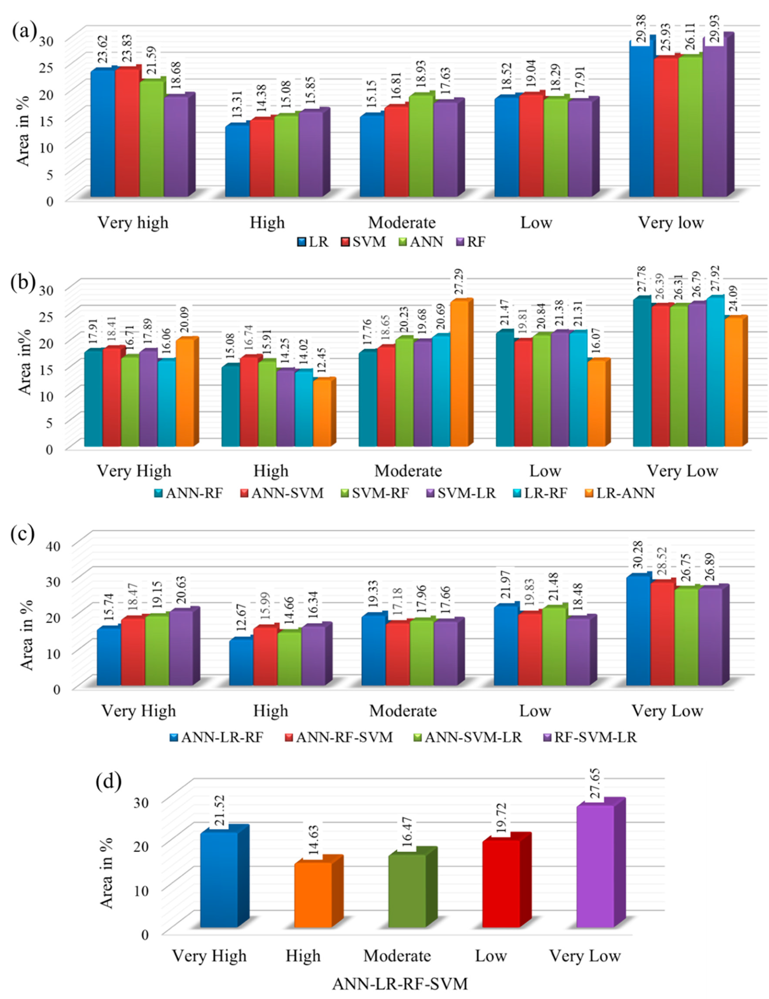
5.2. LSMs by Individual Models

In the first phase of analysis, landslide susceptibility maps (LSMs) were produced applying the single-model based assessment method. Therefore, four different LSMs of the Rudraprayag district were produced by random forest, artificial neural network, support vector machine and logistic regression models individually. All the models were functioned in ‘R studio’ using R programming along with SPSS v17. For all the models, the susceptibility was categorised into five classes based on Jenk’s natural breaks classification algorithm such as Very-high (VH), High (H), Moderate (M), Low (L) and Very-low (VL). For the classification of LSMs into VH, H, M, L, and VL, four techniques were tested, i.e., geometric interval, natural breaks, equal interval, and quantile. The calibration results provided by the Jenk’s natural break are more prominent in distributing landslides as it has no bias and minimum deviation in intra-class and maximum deviation in inter-class which was also found in the work of Arabameri et al. [78].

RF model based LSM (Figure 5b) is categorised into 18.68%, 15.85%, 17.63%, 17.91%, and 29.93% area of the district under VH, H, M, L, and VL classes, respectively. Random forest was fabricated by the relative weight of the mean decrease in accuracy of the Gini index. The ANN model produced 21.59%, 15.08%, 18.93%, 18.29%, and 26.11% areas are susceptible under VH, H, M, L, VL categories, accordingly (Figure 5a). Similarly, the LR model-based result categorized 23.62% area of the district as very highly susceptible, 13.31% as highly susceptible and 15.15%, 18.52%, and 29.38% areas as moderate, low, and very-low category, respectively (Figure 5c). In the case of the SVM model-based LSM (Figure 5d), the very-low (25.93%) and moderate (16.81%) susceptibility class cover the largest areas of the district respectively followed by very-high (23.83%), high (14.38%) and low susceptibility (25.93%) classes. The comparative visualization of the individual model based LSMs are represented in Figure 6.

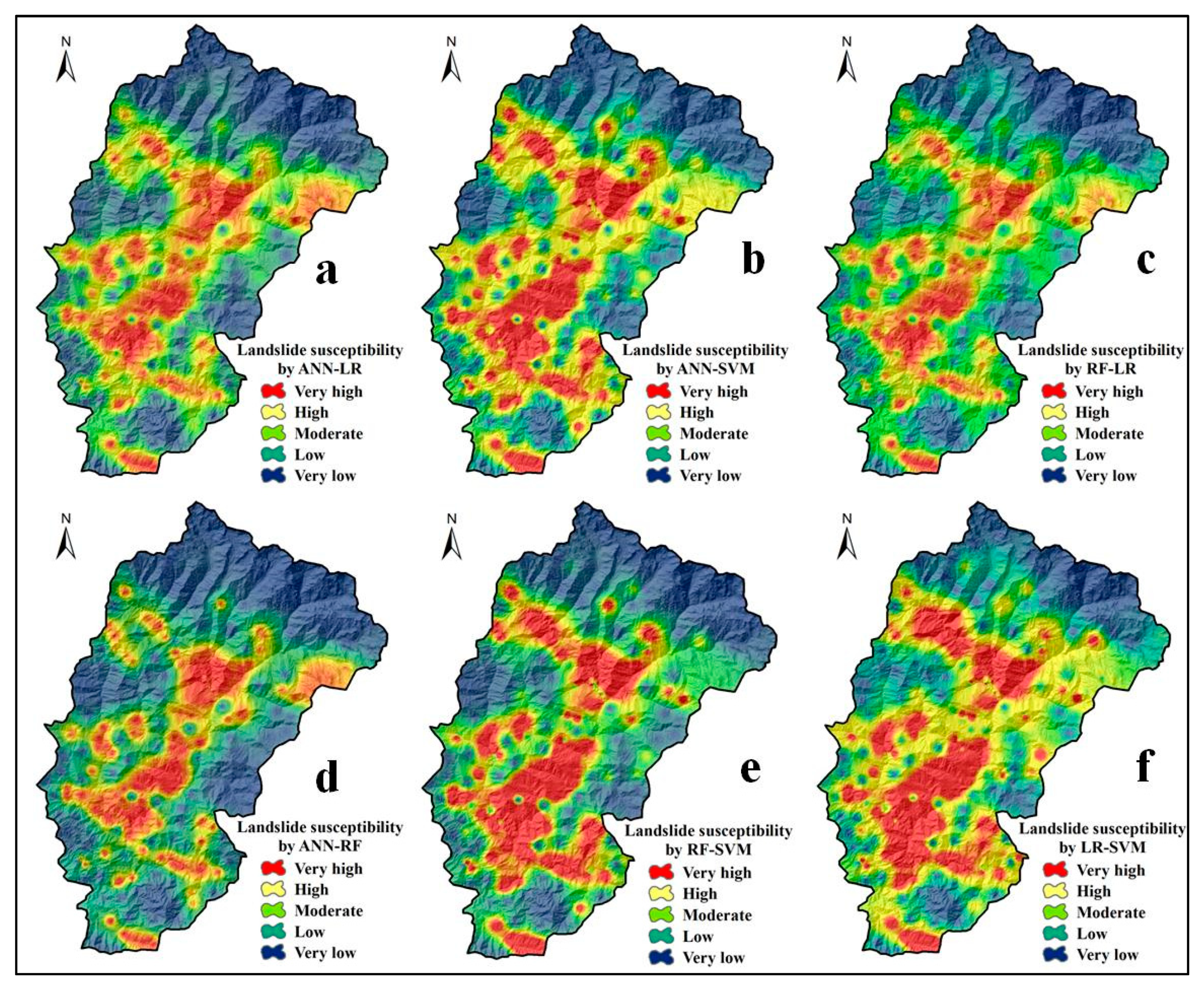
5.3. LSMs by Two Ensemble Models

The second phase of the analysis was to produce LSMs using an ensemble of two-models (Figure 7). Considering each of RF, ANN, LR and SVM model, a set of six ensemble models were derived, i.e., ANN-RF, ANN-SVM, SVM-RF, SVM-LR, LR-RF, and LR-ANN. and the derived LSMs showed varied results. The areal expansion of VH susceptibility class extracted by ANN-RF, ANN-SVM, SVM-RF, SVM-LR, LR-RF and LR-ANN ensemble model are 17.91%, 18.41%, 16.71%, 17.89%, 16.06%, and 20.09% of the total area, respectively. Regarding high susceptibility category, the areas are 15.08%, 16.74%, 15.91%, 14.25%, 14.02%, and 12.45%, respectively for each of the models. The largest area under the moderate category was shown by the LR-ANN model (27.29%) followed by LR-RF (20.69%), SVM-RF (20.23%), SVM-LR (19.68%), ANN-SVM (18.65%), and ANN-RF (17.76%) models. Correspondingly, the total area under L and VL susceptibility classes of the LSMs was 49.25%, 46.2%, 47.15%, 48.17%, 49.23%, and 40.16% accordingly (Figure 6).

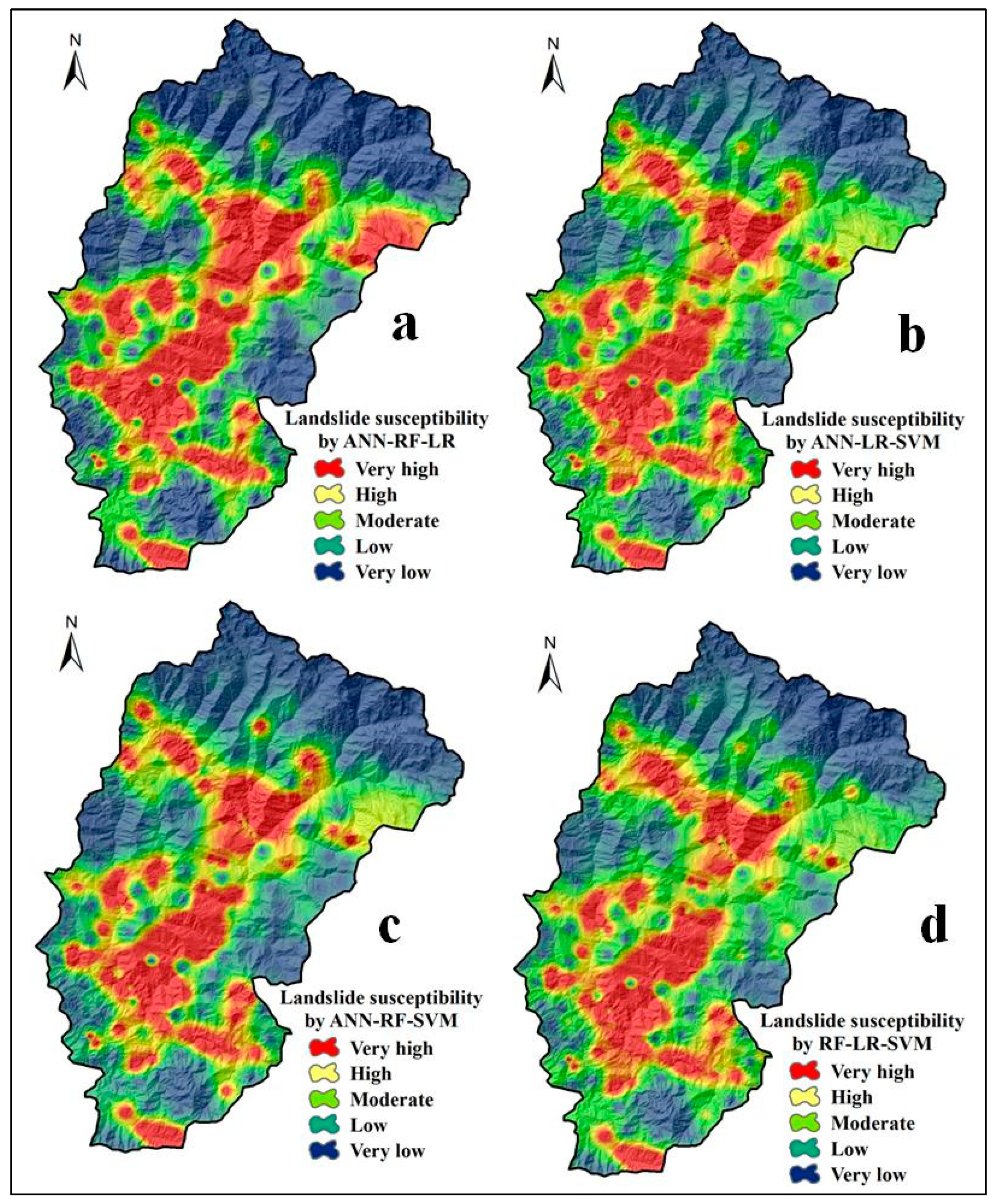
5.4. LSMs by Ensemble of Three-Models

In the third phase, the ensemble approach was executed considering three models differently viz. ANN-LR-RF, ANN-RF-SVM, ANN-SVM-LR, and RF-SVM-LR, which produced four LSMs of the district. The consecutive areal extension of VH, H, M, L, and VL susceptibility classes of derived LSMs was 15.74%, 12.67%, 19.33%, 21.97%, 30.28% of the district by the ANN-LR-RF model (Figure 8a); 18.47%, 15.99%, 17.18%, 19.83%, and 28.52% by the ANN-RF-SVM model (Figure 8c); 19.15%, 14.66%, 17.96%, 21.48%, and 26.75% area by the ANN-SVM-LR model (Figure 8b), and 20.62%, 16.34%, 17.66%, 18.48%, and 26.89% of study area by the RF-SVM-LR model (Figure 8b).

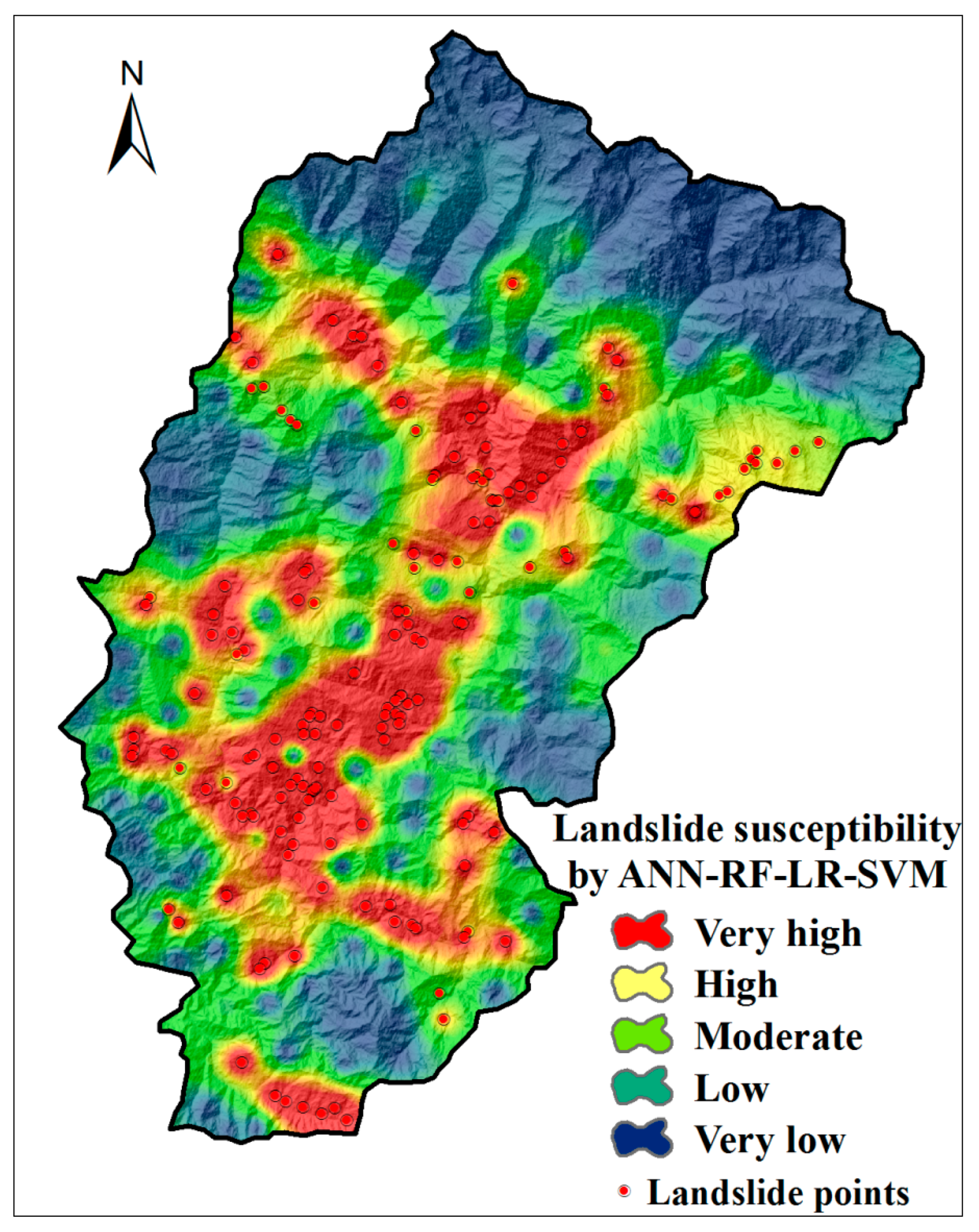
5.5. LSMs by Ensemble of Four-Models

Finally, all four models, i.e., RF, ANN, LR, and SVM models, were combined to prepare the LSM of the Rudraprayag district. The ensemble model of ANN-LR-RF-SVM classified 21.52% area under the very high susceptibility category, 14.63% area under high, 16.47% area under moderate, 19.72% area under low, and 27.65% area of the district under the very low susceptibility category (Figure 9).

5.6. Results of the Validation Techniques

The validation method in this research includes two approaches such as reliability and discrimination ability evaluation. AUCROC, precision and efficiency were computed for measuring the discrimination abilities of the models while the reliability was assessed applying MAE and RMSE which were applied in various research works as validation techniques [79,80,81]. The present research using effective model-based approaches has produced fifteen LSMs considering both single and combined techniques. Therefore, precision, efficiency, AUC, MAE, and RMSE of 15 models using both of the training and testing sub-set GLIs were computed and presented in

Table 4. Results of validation techniques and accuracy prioritization based on training datasets.

Matrix	Training Data Set					Rank					Rank Total	CF	Priority Rank
	Precision	Efficiency	AUC	MAE	RMSE	Precision	Efficiency	AUC	MAE	RMSE
ANN	0.718	0.722	85.12	0.038	0.058	9	9	10	3	3	34	6.8	4
SVM	0.695	0.703	83.39	0.096	0.156	10	10	14	5	6	45	9	11
RF	0.665	0.667	84.59	0.036	0.052	13	13	12	2	2	42	8.4	10
LR	0.636	0.665	82.17	0.237	0.432	15	15	15	13	15	73	14.6	15
ANN-SVM	0.678	0.687	85.07	0.365	0.107	12	12	11	15	5	55	11	12
ANN-LR	0.685	0.69	85.46	0.267	0.249	11	11	8	14	13	57	11.4	13
LR-SVM	0.663	0.683	85.84	0.182	0.266	14	14	6	10	14	58	11.6	14
LR-RF	0.857	0.871	85.48	0.206	0.245	2	2	7	12	12	35	7	6
SVM-RF	0.77	0.785	85.38	0.163	0.069	7	7	9	7	4	34	6.8	5
ANN-RF	0.775	0.789	84.01	0.093	0.168	6	6	13	4	7	36	7.2	8
ANN-LR-SVM	0.766	0.784	86.95	0.182	0.231	8	8	4	9	10	39	7.8	9
ANN-RF-SVM	0.791	0.796	86.73	0.191	0.242	4	4	5	11	11	35	7	7
RF-SVM-LR	0.846	0.861	87.38	0.165	0.215	3	3	3	8	9	26	5.2	2
ANN-LR-RF	0.871	0.878	87.83	0.016	0.019	1	1	1	1	1	5	1	1
ANN-RF-SVM-LR	0.784	0.804	87.76	0.151	0.195	5	5	2	6	8	26	5.2	3

and

Table 5. Results of validation techniques and accuracy prioritization based on testing datasets.

Matrix	Testing Data Set					Rank					Rank Total	CF	Priority Rank
	Precision	Efficiency	AUC	MAE	RMSE	Precision	Efficiency	AUC	MAE	RMSE
ANN	0.817	0.838	86.45	0.027	0.164	7	6	13	1	7	34	6.8	5
SVM	0.785	0.792	85.63	0.067	0.125	9	10	14	2	2	37	7.4	7
RF	0.667	0.708	86.95	0.085	0.146	14	14	11	4	4	47	9.4	10
LR	0.825	0.829	84.7	0.131	0.18	5	8	15	9	10	47	9.4	11
ANN-SVM	0.715	0.723	87.45	0.302	0.387	12	12	9	15	15	63	12.6	15
ANN-LR	0.705	0.709	86.69	0.139	0.186	13	13	12	10	11	59	11.8	14
LR-SVM	0.667	0.708	87.62	0.228	0.0287	15	15	8	14	1	53	10.6	13
LR-RF	0.748	0.77	86.98	0.102	0.159	11	11	10	6	6	44	8.8	9
SVM-RF	0.859	0.881	88.69	0.189	0.217	3	5	7	13	12	40	8	8
ANN-RF	0.821	0.885	89.91	0.109	0.164	6	4	5	7	8	30	6	4
ANN-LR-SVM	0.785	0.812	89.77	0.163	0.275	10	9	6	11	14	50	10	12
ANN-RF-SVM	0.857	0.889	92.03	0.172	0.241	4	3	4	12	13	36	7.2	6
RF-SVM-LR	0.815	0.835	92.29	0.089	0.149	8	7	3	5	5	28	5.6	3
ANN-LR-RF	0.878	0.893	93.98	0.117	0.138	1	1	1	8	3	14	2.8	1
ANN-RF-SVM-LR	0.873	0.889	92.63	0.0761	0.172	2	2	2	3	9	18	3.6	2

and Figure 10. The prioritization results of the models found best success rate (using training GLIs) of ANN-LR-RF model as it ranked 1 (precision = 0.871, efficiency = 0.878, AUC = 87.83, MAE = 0.016, RMSE = 0.019) through compound factor (CF) analysis. Furthermore, in the case of prediction ability (using testing GLIs), the prioritization results also assigned rank 1 for the ANN-LR-RF model (precision = 0.878, efficiency = 0.893, AUC = 93.98, MAE = 0.117, RMSE = 0.138) which confirmed the best fit of this model in the current research of mapping LSS in Rudraprayag district of Uttarakhand, India.

5.7. Result of Variable Importance Analysis

The results of the assessment of the variable importance based on the mean decrease of Gini coefficient using RF model are shown in Figure 11. In addition, the coefficients of logistic regression which also indicates the importance of the variables are shown in

Table 6. Logistic regression coefficients of landslide causative factors.

Landslide Causative Factors	Coefficients of Logistic Regression (B)	Landslide Causative Factors	Coefficients of Logistic Regression (B)
Altitude	1.461	Geology (Gneiss-magmatites)	0.122
Slope	0.028	Geology (Tourmail granite)	2.478
Aspect (Flat)	−1.185	Geology (Chail-Ranghat)	−3.412
Aspect (North)	−0.179	Geology (Granite 500Ma)	−1.744
Aspect (North-east)	0.348	Geology (Salkhlas)	1.062
Aspect (East)	−0.447	Geology (Shail Deoban)	−0.513
Aspect (South-east)	0.531	Geology (Nagthal)	−1.185
Aspect (South)	−0.632	Geology (Chadpur)	−0.179
Aspect (South-west)	−1.185	Geology (Chamoli Qz)	0.348
Aspect (West)	−1.32	Earthquake zone (High)	0.348
Aspect (North-West)	−2.199	Earthquake zone (Moderate)	−0.447
Curvature	0.976	Major Road density	1.241
SPI	0.026	NDVI	−0.005
Rainfall	1.076	LULC (Graz area)	0.078
Drainage density	1.016	LULC (Evergreen forest)	−0.048
TWI	0.034	LULC (Perennial water)	0.122
Soil depth	0.084	LULC (Settlement)	2.478
Soil texture (Very fine)	−0.334	LULC (Cropland)	1.412
Soil texture (Loamy skeletal)	1.476	LULC (Barren land)	−1.744
Soil texture (Sandy skeletal)	−1.194	LULC (Scrub forest)	1.062
Soil texture (Mixed loamy)	1.445	LULC (Deciduous forest)	−0.513
Soil texture (Fine loamy)	−0.119	LULC (Seasonal water)	−1.185
Soil texture (Granular loamy)	1.114	LULC (Glacial area)	−0.513
Distance from lineament	1.102	LULC (Permanent snow)	−1.185

. As Figure 11 shows, all the causative factors generally contributed to the landslide susceptibility model. However, altitude is the most important factor, followed by drainage density, road density, lineament density and slope respectively. Like the mean decrease of Gini, the coefficients of logistic regression (Table 6) also indicate a strong relationship between the landslide occurrence and the altitude, rainfall, drainage density, road density and distance from lineament. These results showed that most of the landslides occurred in elevated areas with high drainage density and road density.

6. Discussion

Determining the LCFs, generation of LSMs and selection of the best-fitted model is the initial stage of landslide hazard assessment and the present research was intended to attempt that. As the landslide is the uncertainty of spatial association among the several factors, different models can be applied for the prediction. During the last decades, various empirical and numerical models have been attempted to forecast geohazards [14,79,82]. However, those models have some limitations and assumptions [15,24]. Recently, data mining models have been largely popularised in the research community, especially in modelling different environmental risks due to their ability to analyse complex connection between predictors (LCFs) and responses (landslide or non-landslide). Besides this, the ensemble of different data mining models along with statistical models also has been used effectively to produce LSMs [13,63,83]. This work was carried out through four phases of ensemble approaches that made the work novel compared to other works. In resolving the over-fitting problem, an ensemble of these machine learning models has more capability because these models automate the task of selecting multiple datasets without pre-assumption and can handle massive data [77]. Furthermore, the evaluation of the prediction ability of the models is a fundamental phase in any modelling work and it could be judged using both threshold dependent and independent methods [14,83]. Therefore, the AUC, precision, efficiency, MAE, and RMSE of each modelling approach were assessed considering both the training sub-set GLIs and testing or validation sub-set GLIs. Measurement of AUC including training sub-set represents success rate while the prediction rate was computed using testing sub-set of GLIs [14,73].

Considering the training sub-set GLIs, in the individual modelling, the AUC was found highest (85.12%) in ANN model followed by RF (84.59%), SVM (83.39%) and LR (82.17%) model (Table 4). In terms of precision and efficiency values, ANN leads the highest performance followed by SVM, RF and LR model (Table 4). However, both the reliability measures MAE and RMSE showed best results for RF model followed by ANN, SVM and LR model (Table 4). LR-RF showed the best result in terms of precision and efficiency when two models were combined and all the two-model ensembles have shown greater accuracy than the individual model in term of AUC (Figure 10). When the three models were combined, ANN-LR-RF revealed the best result under each measure of precision (0.871), efficiency (0.878), AUC (87.83%), MAE (0.016) and RMSE (0.019) (Table 4). At the last phase, to produce LSM, all four models were combined and the performances of the ensemble ANN-RF-SVM-LR model were: precision = 0.784, efficiency = 0.804, AUC = 87.76%, MAE = 0.151, and RMSE = 0.195. Correspondingly, the performances (reliability and discrimination ability) of the models were assessed considering testing sub-set of GLIs as well. Individually, the LR model regarded as the best in terms of precision (0.825) and efficiency (0.829) but AUC defined the RF model as the best fit for predicting landslide susceptibility. The RF model has greater acceptability in spatial risk mapping as found in various research works [30,54,78]. Similarly, the validation results of two-model ensemble, three-model ensemble and four-model ensemble have been listed in Table 5.

Compound factor-based prioritization of models in terms of the discrimination and reliability accuracy measures considering training and testing datasets was used to find the best-fitted models. Regarding the success rate of the produced LSMs, the CF method showed that an ensemble of ANN-LR-RF models was the best fit followed by RF-SVM-LR and ANN-RF-SVM-LR models, respectively. In the context of prediction performance, priority was the highest for ANN-LR-RF again followed by ANN-RF-SVM-LR and RF-SVM-LR models. The produced LSMs by the individual and ensemble models were classified into five susceptibility classes. The areas covering different susceptibility classes were varied from model to model. The best fit ensemble model, i.e., ANN-LR-RF showed that 15.74%, 12.67%, 19.33%, 21.97%, and 30.28% areas have VH, H, M, L, and VL susceptibility for the landslide. However, the output of the work will help the planners for the management of landslide in this area.

7. Conclusions

The key field of concern in this study is the analysis of landslide susceptibility. Single and ensemble models were successfully used for landslide susceptibility evaluation in the Rudraprayag district of Garhwal Himalaya. ROC curve, efficiency, accuracy, MAE, and RMSE were employed to assess and compare these LSS models. Finally, using the CF the best model was selected. The findings of the validation techniques show that the LSS models prepared by ANN, FR, SVM, LR, and their ensembles performed well in this analysis. The ensemble of ANN, RF, SVM, and LR models played an improving role as they improved the values of AUC. However, with respect to the results of robustness, the ANN-RF-LR ensemble had the highest reliability in terms of results where the highest agreement was found in the efficiency, accuracy, AUC of success rate curve, and predictive rate curve values, MAE and RMSE. The present research shows that ensemble models are effective tools that could be used in landslide prediction and landslide management for efficient decision-making by the authorities. In the present analysis, these models were utilized in the Rudraprayag district. However, for wider use, the output of such models may be used for areas of similar geo-environmental conditions. The key drawback of this analysis is that we used a limited set of LCFs and a fixed training testing samples dataset ratio (70:30) for the all the models. The performance of the models will have to be further tested through a variety of training and testing sets of sample datasets as well as LCF sets.

References

1. IAEG Commission on Landslides. Suggested nomenclature for landslides. Bull. Int. Assoc. Eng. Geol. 1990, 41, 3–16. [Google Scholar]
2. Nadim, F.; Kjekstad, O.; Peduzzi, P. Global landslide and avalanche hotspots. Landslides 2006, 3, 159–173. [Google Scholar] [CrossRef]
3. Geertsema, M.; Highland, L.; Vaugeouis, L. Environmental impact of landslides. In Landslides–Disaster Risk Reduction; Springer: Berlin, Germany, 2009; pp. 589–607. [Google Scholar]
4. Faiz, M.A.; Liu, D.; Fu, Q.; Sun, Q.; Li, M.; Baig, F.; Li, T.; Cui, S. How accurate are the performances of gridded precipitation data products over Northeast China? Atmos. Res. 2018, 211, 12–20. [Google Scholar]
5. Raman, R.; Punia, M. The application of GIS-based bivariate statistical methods for landslide hazards assessment in the upper Tons river valley, Western Himalaya, India. Georisk: Assess. Manag. Risk Eng. Syst. Geohazards 2012, 6, 145–161. [Google Scholar]
6. Ray, P.C.; Parvaiz, I.; Jayangondaperumal, R.; Thakur, V.C.; Dadhwal, V.K.; Bhat, F.A. Analysis of seismicity-induced landslides due to the 8 October 2005 earthquake in Kashmir Himalaya. Curr. Sci. 2009, 25, 1742–1751. [Google Scholar]
7. Ghosh, S.; Chakraborty, I.; Bhattacharya, D. Generating field-based inventory of earthquake-induced landslides in the Himalayas—An aftermath of the 18 September 2011 Sikkim earthquake. Indian J. Geosci. 2012, 66, 27–38. [Google Scholar]
8. Maheshwari, B.K. Earthquake-induced landslide hazard assessment of chamoli district, uttarakhand using relative frequency ratio method. Indian Geotech. J. 2019, 49, 108–123. [Google Scholar] [CrossRef]
9. Moreiras, S.M. Landslide susceptibility zonation in the Rio Mendoza Valley, Argentina. Geomorphology 2005, 66, 345–357. [Google Scholar]
10. Wadhawan, S.K. Landslide susceptibility mapping, vulnerability and risk assessment for development of early warning systems in India. In Landslides: Theory, Practice and Modelling; Springer: Cham, Switzerland, 2019; pp. 145–172. [Google Scholar]
11. Choi, J.; Oh, H.J.; Lee, H.J.; Lee, C.; Lee, S. Combining landslide susceptibility maps obtained from frequency ratio, logistic regression, and artificial neural network models using ASTER images and GIS. Eng. Geol. 2011, 124, 12–23. [Google Scholar] [CrossRef]
12. Youssef, A.M.; Pradhan, B.; Jebur, M.N.; El-Harbi, H.M. Landslide susceptibility mapping using ensemble bivariate and multivariate statistical models in Fayfa area, Saudi Arabia. Environ. Earth Sci. 2014, 73, 3745–3761. [Google Scholar]
13. Chen, W.; Pourghasemi, H.R.; Zhao, Z. A GIS-based comparative study of Dempster-Shafer, logistic regression and artificial neural network models for landslide susceptibility mapping. Geocarto Int. 2017, 32, 367–385. [Google Scholar] [CrossRef]
14. Pradhan, B. A comparative study on the predictive ability of the decision tree, support vector machine and neuro-fuzzy models in landslide susceptibility mapping using GIS. Comput. Geosci. 2013, 51, 350–365. [Google Scholar] [CrossRef]
15. Chen, W.; Xie, X.; Wang, J.; Pradhan, B.; Hong, H.; Bui, D.T.; Duan, Z.; Ma, J. A comparative study of logistic model tree, random forest, and classification and regression tree models for spatial prediction of landslide susceptibility. Catena 2017, 151, 147–160. [Google Scholar] [CrossRef] [Green Version]
16. Raja, N.B.; Çiçek, I.; Türkoğlu, N.; Aydin, O.; Kawasaki, A. Landslide susceptibility mapping of the Sera River basin using logistic regression model. Nat. Hazards 2017, 85, 1323–1346. [Google Scholar] [CrossRef] [Green Version]
17. Tsangaratos, P.; Ilia, I.; Hong, H.; Chen, W.; Xu, C. Applying information theory and GIS-based quantitative methods to produce landslide susceptibility maps in Nancheng County, China. Landslide 2017, 14, 1091–1111. [Google Scholar]
18. Goetz, J.; Brenning, A.; Petschko, H.; Leopold, P. Evaluating machine learning and statistical prediction techniques for landslide susceptibility modeling. Comput. Geosci. 2015, 81, 1–11. [Google Scholar] [CrossRef]
19. Hong, H.; Pourghasemi, H.R.; Pourtaghi, Z.S. Landslide susceptibility assessment in Lianhua County (China): A comparison between a random forest data mining technique and bivariate and multivariate statistical models. Geomorphology 2016, 259, 105–118. [Google Scholar] [CrossRef]
20. Shirzadi, A.; Bui, D.T.; Pham, B.T.; Solaimani, K.; Chapi, K.; Kavian, A.; Shahabi, H.; Revhaug, I. Shallow landslide susceptibility assessment using a novel hybrid intelligence approach. Environ. Earth Sci. 2017, 76, 60. [Google Scholar] [CrossRef]
21. Tsangaratos, P.; Ilia, I. Landslide susceptibility mapping using a modified decision tree classifier in the Xanthi Perfection, Greece. Landslides 2016, 13, 305–320. [Google Scholar] [CrossRef]
22. Dou, J.; Yamagishi, H.; Pourghasemi, H.R.; Yunus, A.P.; Song, X.; Xu, Y.; Zhu, Z. An integrated artificial neural network model for the landslide susceptibility assessment of Osado Island, Japan. Nat. Hazards 2015, 78, 1749–1776. [Google Scholar]
23. Benediktsson, J.; Swain, P.H.; Ersoy, O.K. Neural network approaches versus statistical methods in classification of multisource remote sensing data. IEEE T Geosci Remote 1990, 28, 540–552. [Google Scholar]
24. Tehrany, M.S.; Pradhan, B.; Jebur, M.N. Spatial prediction of flood susceptible areas using rule based decision tree (DT) and a novel ensemble bivariate and multivariate statistical models in GIS. J. Hydrol. 2014, 504, 69–79. [Google Scholar] [CrossRef]
25. Hembram, T.K.; Paul, G.C.; Saha, S. Modelling of gully erosion risk using new ensemble of conditional probability and index of entropy in Jainti River basin of Chotanagpur Plateau Fringe Area, India. Appl. Geomat. 2020, 1–24. [Google Scholar] [CrossRef]
26. Pourghasemi, H.R.; Yousefi, S.; Kornejady, A.; Cerdà, A. Performance assessment of individual and ensemble data-mining techniques for gully erosion modeling. Sci. Total Environ. 2017, 609, 764–775. [Google Scholar] [CrossRef] [PubMed] [Green Version]
27. Barzegar, R.; Moghaddam, A.A.; Deo, R.; Fijani, E.; Tziritis, E. Mapping groundwater contamination risk of multiple aquifers using multi-model ensemble of machine learning algorithms. Sci. Total Environ. 2018, 621, 697–712. [Google Scholar] [CrossRef] [PubMed]
28. Naghibi, S.A.; Pourghasemi, H.R.; Dixon, B. GIS-based groundwater potential mapping using boosted regression tree, classification and regression tree, and random forest machine learning models in Iran. Environ. Monit. Assess. 2016, 188, 44. [Google Scholar]
29. Mojaddadi, H.; Pradhan, B.; Nampak, H.; Ahmad, N.; Ghazali, A.H.B. Ensemble machine-learning-based geospatial approach for flood risk assessment using multi-sensor remote-sensing data and GIS. Geomat. Nat. Hazards Risk 2017, 8, 1080–1102. [Google Scholar] [CrossRef] [Green Version]
30. Kadavi, P.R.; Lee, C.W.; Lee, S. Application of ensemble-based machine learning models to landslide susceptibility mapping. Remote Sens. 2018, 10, 1252. [Google Scholar] [CrossRef] [Green Version]
31. Aghdam, I.N.; Varzandeh, M.H.M.; Pradhan, B. Landslide susceptibility mapping using an ensemble statistical index (Wi) and adaptive neuro-fuzzy inference system (ANFIS) model at Alborz Mountains (Iran). Environ. Earth Sci. 2016, 75, 553. [Google Scholar]
32. The Pioneer. Available online: https://www.dailypioneer.com/2019/state-editions/landslide-at-rudraprayag-kills-8.html (accessed on 21 October 2019).
33. Indian Meteorological Department. Available online: https://mausam.imd.gov.in/ (accessed on 24 November 2019).
34. US Geological Survey Earthexplorer. Available online: https://earthexplorer.usgs.gov/ (accessed on 20 December 2019).
35. Bhuvan. Available online: http://bhuvan.nrsc.gov.in/ (accessed on 22 December 2019).
36. Yilmaz, C.; Topal, T.; Suzen, M.L. GIS-based landslide susceptibility mapping using bivariate statistical analysis in Devrek (Zonguldak-Turkey). Environ. Earth Sci. 2012, 65, 2161–2178. [Google Scholar] [CrossRef]
37. Van Westen, C.J.; van Asch, T.W.J.; Soeters, R. Landslide hazard and risk zonation—Why is it still so difficult? Bull. Eng. Geol. Environ. 2006, 65, 167–184. [Google Scholar] [CrossRef]
38. Kononenko, I. Estimating attributes: Analysis and extensions of RELIEF. In European Conference on Machine Learning; Springer: Berlin/Heidelberg, Germany, 1994; pp. 171–182. [Google Scholar]
39. Wang, L.-J.; Guo, M.; Sawada, K.; Lin, J.; Zhang, J. A comparative study of landslide susceptibility maps using logistic regression, frequency ratio, decision tree, weights of evidence and artificial neural network. Geosci. J. 2016, 20, 117–136. [Google Scholar] [CrossRef]
40. Pham, B.T.; Bui, D.T.; Prakash, I.; Dholakia, M. Hybrid integration of Multilayer Perceptron Neural Networks and machine learning ensembles for landslide susceptibility assessment at Himalayan area (India) using GIS. Catena 2017, 149, 52–63. [Google Scholar]
41. Pham, B.T.; Jaafari, A.; Prakash, I.; Bui, D.T. A novel hybrid intelligent model of support vector machines and the MultiBoost ensemble for landslide susceptibility modeling. Bull. Eng. Geol. Environ. 2019, 76, 2865–2886. [Google Scholar]
42. Li, Z.; Zhu, Q.; Gold, C. Digital Terrain Modeling: Principles and Methodology; CRC Press: Boca Raton, FL, USA, 2005. [Google Scholar]
43. Wentworth, C.K. A simplified method of determining the average slope of land surfaces. Am. J. Sci. 1930, 117, 184–194. [Google Scholar]
44. Burrough, P.A.; McDonell, R.A. Principles of Geographical Information Systems; Oxford University Press: New York, NY, USA, 1998; p. 190. [Google Scholar]
45. Moore, I.D.; Grayson, R.B.; Ladson, A.R. Digital terrain modelling: A review of hydrological, geomorphological, and biological applications. Hydrol. Process. 1991, 5, 3–30. [Google Scholar] [CrossRef]
46. Bayraktar, H.; Turalioglu, S. A Kriging-based approach for locating a sampling site—In the assessment of airquality. Stoch. Environ. Res. Risk Assess. 2005, 19, 301–305. [Google Scholar] [CrossRef]
47. Moore, I.D.; Burch, G.J. Physical basis of the length slope factor in the universal soil loss equation. Soil Sci. Soc. Am. 1986, 50, 1294–1298. [Google Scholar] [CrossRef]
48. Ay, N.; Amari, S.-I. A novel approach to canonical divergences within information geometry. Entropy 2015, 17, 8111–8129. [Google Scholar] [CrossRef]
49. Chawla, A.; Pasupuleti, S.; Chawla, S.; Rao, A.C.S.; Sarkar, K.; Dwivedi, R. Landslide susceptibility zonation mapping: A case study from darjeeling district, Eastern Himalayas, India. J. Indian Soc. Remote Sens. 2019, 47, 497–511. [Google Scholar]
50. Crippen, R.E. Calculating the vegetation index faster. Remote Sens. Environ. 1990, 34, 71–73. [Google Scholar] [CrossRef]
51. Myung, I.J. Tutorial on maximum likelihood estimation. J. Math. Psychol. 2003, 47, 90–100. [Google Scholar] [CrossRef]
52. Prasad, K.; Gopi, S.; Rao, R. Demarcation of Priority Macro-Watersheds in Mahbubnagar District, AP Using Remote Sensing Techniques; Tata McGraw-Hill: New York, NY, USA, 1992; pp. 263–269. [Google Scholar]
53. Poudyal, C.P.; Chang, C.; Oh, H.-J.; Lee, S. Landslide susceptibility maps comparing frequency ratio and artificial neural networks: A case study from the Nepal Himalaya. Environ. Earth Sci. 2010, 61, 1049–1064. [Google Scholar] [CrossRef]
54. Breiman, L. Random forests. Mach. Learn. 2001, 45, 5–32. [Google Scholar] [CrossRef] [Green Version]
55. Gayen, A.; Pourghasemi, H.R.; Saha, S.; Keesstra, S.; Bai, S. Gully erosion susceptibility assessment and management of hazard-prone areas in India using different machine learning algorithms. Sci. Total Environ. 2019, 668, 124–138. [Google Scholar] [CrossRef] [PubMed]
56. Trigila, A.; Iadanza, C.; Esposito, C.; Scarascia-Mugnozza, G. Comparison of logistic regression and random forests techniques for shallow landslide susceptibility assessment in Giampilieri (NE Sicily, Italy). Geomorphology 2015, 249, 119–136. [Google Scholar] [CrossRef]
57. Micheletti, N.; Foresti, L.; Robert, S.; Leuenberger, M.; Pedrazzini, A.; Jaboyedoff, M.; Kanevski, M. Machine learning feature selection methods for landslide susceptibility mapping. Math. Geosci. 2014, 46, 33–57. [Google Scholar] [CrossRef] [Green Version]
58. Aditian, A.; Kubota, T.; Shinohara, Y. Comparison of GIS-based landslide susceptibility models using frequency ratio, logistic regression, and artificial neural network in a tertiary region of Ambon, Indonesia. Geomorphology 2018, 318, 101–111. [Google Scholar] [CrossRef]
59. Jing, L. A review of techniques, advances and outstanding issues in numerical modelling for rock mechanics and rock engineering. Int. J. Rock Mech. Min. Sci. 2003, 40, 283–353. [Google Scholar] [CrossRef]
60. Yao, X.; Tham, L.G.; Dai, F.C. Landslide susceptibility mapping based on support vector machine: A case study on natural slopes of Hong Kong, China. Geomorphology 2008, 101, 572–582. [Google Scholar] [CrossRef]
61. Rahmati, O.; Tahmasebipour, N.; Haghizadeh, A.; Pourghasemi, H.R.; Feizizadeh, B. Evaluation of different machine learning models for predicting and mapping the susceptibility of gully erosion. Geomorphology 2017, 298, 118–137. [Google Scholar] [CrossRef]
62. Tien Bui, D.; Pradhan, B.; Lofman, O.; Revhaug, I. Landslide susceptibility assessment in Vietnam using support vector machines, decision tree, and Naïve Bayes Models. Math. Probl. Eng. 2012, 2012, 974638. [Google Scholar] [CrossRef] [Green Version]
63. Roy, J.; Saha, S. Landslide susceptibility mapping using knowledge driven statistical models in Darjeeling District, West Bengal, India. Geoenvironmental Disasters 2019, 6, 11. [Google Scholar] [CrossRef] [Green Version]
64. Menard, S. Coefficients of determination for multiple logistic regression analysis. Am. Statistician. 2000, 54, 17–24. [Google Scholar]
65. Akgun, A. A comparison of landslide susceptibility maps produced by logistic regression, multi-criteria decision, and likelihood ratio methods: A case study at İzmir, Turkey. Landslides 2012, 9, 93–106. [Google Scholar] [CrossRef]
66. Rokach, L. Ensemble-based classifiers. Artif. Intell. Rev. 2010, 33, 1–39. [Google Scholar] [CrossRef]
67. Lee, M.J.; Choi, J.W.; Oh, H.J.; Won, J.S.; Park, I.; Lee, S. Ensemble-based landslide susceptibility maps in Jinbu area, Korea. Environ. Earth Sci. 2012, 67, 23–37. [Google Scholar] [CrossRef]
68. Jebur, M.N.; Pradhan, B.; Tehrany, M.S. Optimization of landslide conditioning factors using very high-resolution airborne laser scanning (LiDAR) data at catchment scale. Remote Sens. Environ. 2014, 152, 150–165. [Google Scholar] [CrossRef]
69. Gayen, A.; Saha, S. Application of weights-of-evidence (WoE) and evidential belief function (EBF) models for the delineation of soil erosion vulnerable zones: A study on Pathro river basin, Jharkhand, India. Modeling Earth Syst. Environ. 2017, 3, 1123–1139. [Google Scholar] [CrossRef]
70. Gayen, A.; Saha, S. Deforestation probable area predicted by logistic regression in Pathro river basin: A tributary of Ajay River. Spat. Inf. Res. 2018, 26, 1–9. [Google Scholar] [CrossRef]
71. Frattini, P.; Crosta, G.; Carrara, A. Techniques for evaluating the performance of landslide susceptibility models. Eng. Geol. 2010, 111, 62–72. [Google Scholar] [CrossRef]
72. Hembram, T.K.; Paul, G.C.; Saha, S. Comparative Analysis between Morphometry and Geo-Environmental Factor Based Soil Erosion Risk Assessment Using Weight of Evidence Model: A Study on Jainti River Basin, Eastern India. Environ. Process. 2019, 6, 883–913. [Google Scholar] [CrossRef]
73. Can, T.; Nefeslioglu, H.; Gokceoglu, C.; Sonmez, H.; Duman, T.Y. Susceptibility assessments of shallow earthflows triggered by heavy rainfall at three catchments by logistic regression analysis. Geomorphology 2005, 72, 250–271. [Google Scholar] [CrossRef]
74. Altaf, S.; Meraj, G.; Ahmad Romshoo, S. Morphometry and land cover based multicriteria analysis for assessing the soil erosion susceptibility of the western Himalayan watershed. Environ. Monit. Assess. 2014, 186, 8391–8412. [Google Scholar] [CrossRef]
75. Hembram, T.K.; Saha, S. Prioritization of sub-watersheds for soil erosion based on morphometric attributes using fuzzy AHP and compound factor in Jainti River basin, Jharkhand, Eastern India. Environ. Dev. Sustain. 2018, 22, 1241–1268. [Google Scholar]
76. Kutlug Sahin, E.; Ipbuker, C.; Kavzoglu, T. Investigation of automatic feature weighting methods (Fisher, Chi-square and Relief-F) for landslide susceptibility mapping. Geocarto Int. 2017, 32, 956–977. [Google Scholar]
77. Tien Bui, D.; Shahabi, H.; Shirzadi, A.; Chapi, K.; Pradhan, B.; Chen, W.; Khosravi, K.; Panahi, M.; Bin Ahmad, B.; Saro, L. Land subsidence susceptibility mapping in south korea using machine learning algorithms. Sensors 2018, 18, 2464. [Google Scholar]
78. Pradhan, B. Flood susceptible mapping and risk area delineation using logistic regression, GIS and remote sensing. J. Spat Hydrol. 2010, 9, 1–18. [Google Scholar]
79. Conoscenti, C.; Angileri, S.; Cappadonia, C.; Rotigliano, E.; Agnesi, V.; Märker, M. Gully erosion susceptibility assessment by means of GIS-based logistic regression: A case of Sicily (Italy). Geomorphology 2014, 204, 399–411. [Google Scholar] [CrossRef] [Green Version]
80. Lombardo, L.; Cama, M.; Conoscenti, C.; Märker, M.; Rotigliano, E. Binary logistic regression versus stochastic gradient boosted decision trees in assessing landslide susceptibility for multiple-occurring landslide events: Application to the 2009 storm event in Messina (Sicily, southern Italy). Nat. Hazards 2015, 79, 1621–1648. [Google Scholar]
81. Suzen, M.L.; Doyuran, V. A comparison of the GIS based landslide susceptibility assessment methods: Multivariate versus bivariate. Environ. Geol. 2004, 45, 665–679. [Google Scholar]
82. Arabameri, A.; Pradhan, B.; Rezaei, K.; Sohrabi, M.; Kalantari, Z. GIS-based landslide susceptibility mapping using numerical risk factor bivariate model and its ensemble with linear multivariate regression and boosted regression tree algorithms. J. Mt. Sci. 2019, 16, 595–618. [Google Scholar] [CrossRef]
83. Glade, T.; Crozier, M.J. Landslide hazard and risk: Concluding comment and perspectives. In Landslide Hazard Risk; Wiley: Chichester, UK, 2005; pp. 767–774. [Google Scholar]
Figure 1. Location map of the study area with landslides.
Applsci 10 03772 g001
Figure 2. Methodological flow diagram of the present research. SPI (stream power index); TWI (topographical wetness index); NDVI (normalized difference vegetation index); LU/LC (land use /land cover).
Applsci 10 03772 g002
Figure 3. Field photographs showing some landslides in the study area: (a). Rudraprayag Gouri-kund Highway (30°34’09” N & 79°07’38” E), (b). Amar Jwala (30°38’09” N & 78°57’38” E), (c). Chandi-kadhar (30°29’13” N & 78°55’07” E) and (d) Chardham Rought, Janki Chatti Area (30°20’22” N & 78°58’13” E).
Applsci 10 03772 g003
Figure 4. Landslide conditioning factors: (a) elevation, (b) slope steepness, (c) slope aspect, (d) curvature, (e) stream power index, (f) rainfall, (g) drainage density, (h) topographical wetness index, (i) soil depth, (j) soil texture, (k) distance to lineaments, (l) geology, (m) seismic zone, (n) road density, (o) NDVI, and (p) land use/land cover (LU/LC).
Applsci 10 03772 g004aApplsci 10 03772 g004bApplsci 10 03772 g004c
Figure 5. Landslide susceptibility mapping using single models: (a) ANN (b) RF, (c) LR and (d) SVM.
Applsci 10 03772 g005
Figure 6. Distribution of area under different landslide susceptibility classes (in %) of (a) individual models, (b) ensemble of two models, (c) ensemble of three models and (d) ensemble of four models.
Applsci 10 03772 g006
Figure 7. Landslide susceptibility mapping using ensemble of two models: (a) ANN-LR, (b) ANN-SVM, (c) LR-RF, (d) ANN-RF, (e) SVM-RF, and (f) LR-SVM.
Applsci 10 03772 g007
Figure 8. Landslide susceptibility mapping using ensemble of three models: (a) ANN-LR-RF, (b) ANN-LR-SVM, (c) ANN-RF-SVM, and (d) RF-SVM-LR.
Applsci 10 03772 g008
Figure 9. Landslide susceptibility mapping using ensemble of ANN-RF-SVM-LR.
Applsci 10 03772 g009
Figure 10. Area under the curves based on training datasets (success rate curve): (a) individual models, (b) ensemble of two models, and (c) ensemble of three or four ensemble models; based on validation datasets (prediction rate curve): (d) individual models, (e) ensemble of two models, and (f) ensemble of three or four ensemble models.
Applsci 10 03772 g010
Figure 11. Weights of landslide causative factors calculated by RF.
Applsci 10 03772 g011