Lanchester Models for Irregular Warfare

Operations Research Department, Naval Postgraduate School, Monterey, CA 93943, USA
Mathematics 2020, 8(5), 737; https://doi.org/10.3390/math8050737
Submission received: 25 March 2020
/
Revised: 2 May 2020
/
Accepted: 4 May 2020
/
Published: 7 May 2020
(This article belongs to the Special Issue Mathematical Models in Security, Defense, Cyber Security and Cyber Defense)
Abstract
:Military operations research and combat modeling apply mathematical models to analyze a variety of military conflicts and obtain insights about these phenomena. One of the earliest and most important set of models used for combat modeling is the Lanchester equations. Legacy Lanchester equations model the mutual attritional dynamics of two opposing military forces and provide some insights regarding the fate of such engagements. In this paper, we review recent developments in Lanchester modeling, focusing on contemporary conflicts in the world. Specifically, we present models that capture irregular warfare, such as insurgencies, highlight the role of target information in such conflicts, and capture multilateral situations where several players are involved in the conflict (such as the current war in Syria).
1. Introduction
Military operations research and combat modeling apply mathematical models to analyze a variety of military conflicts and combat situations, and obtain insights about these phenomena [1,2]. One of the earliest and most important set of models used for combat modeling is the Lanchester equations [3]. While there are two major manifestations of Lanchester equations—deterministic and stochastic—we focus in this paper only on the deterministic equations.
Lanchester equations are systems of ordinary differential equations describing the mutual attrition that occurs continuously in time between two opposing forces engaged in violent confrontation. The equations involve state variables that represent the number of live combatants (or weapons) at any given time during the battle. Each equation expresses the rate of change in one state variable as a function of other state variables. There are several Lanchester models that differ in their underlying assumptions regarding the operational posture and/or the tactical situation. We describe the two most common models in Section 2.
Lanchester equations, and variations thereof, have been implemented in large-scale combat models [4,5] and used by military analysts and combat planners for studying force structure and combat courses of action.
The recent literature on Lanchester equations is quite wide in scope and ranges from fitting Lanchester models to data from historical battles [6,7,8], to using partial differential equations to capture spatial and interaction effects [9], and to developing approximate solutions to stochastic versions of Lanchester equations [10]. Lanchester models have also been used in biology [11], evolution [12], and even in the advertisement world [13] and video-gaming [14].
A particular body of research on Lanchester models, notable in the past ten years or so, focuses on irregular warfare, which is manifested in asymmetric conflicts such as insurgencies and multilateral engagements. Irregular warfare is also characterized by asymmetry in the mechanism that provides information, intelligence and situational awareness to the two sides. These types of irregular warfare represent most recent conflicts, such as those in Afghanistan and Syria.
In this paper, we review recent applications of Lanchester theory to irregular warfare. One type of application includes Lanchester models in which the situational awareness capabilities on both sides are asymmetric; one side can target better than the other and therefore gains an advantage. A second type of model relates to cases where the two sides of the conflict are profoundly different in terms of their force structures and their associated attritional dynamics. Such models describe many-on-one situations or scenarios where civilians have a significant effect on the way the conflict evolves. A third type of irregular conflict is when there are more than two sides competing for dominance. We call such conflicts multilateral conflicts. Consider a situation where several sides, Blue, Red, Brown, Green, etc., seek dominance in a region by fighting (or cooperating with) others. Such multilateral conflicts lend themselves to game-theoretic situation, which we discuss in this paper. A striking result characterizes the fate of such conflicts (see Section 6).
The paper is organized as follows: in Section 2, we present a brief introduction to Lanchester models, describing the legacy aimed-fire and un-aimed (area) fire models [3], as well as the ancient battle. Section 3 presents models that capture asymmetric battles such as insurgencies and one-on-many combat situations. In particular, we present the classical guerrilla model of Deitchman [15]. Section 4 focuses on the role of information and combat intelligence in Lanchester modeling. Section 5 describes Lanchester models that incorporate the presence of civilians during insurgencies and show their impact on tactics and battlefield outcomes. Section 6 presents two models of a multilateral conflict such as the one that has been going on for the past nine years in Syria. Section 7 summarizes the paper and points at some future research directions in Lanchester theory.
2. Legacy Lanchester Models
Frederick William Lanchester proposed in 1916 to model mutual attrition of two fighting forces by a set of ordinary differential equations (ODE) [3]. The state variables of the ODE represent fighting entities in the battlefield, and each of the ODEs capture the rate of decrease in a certain state variable as a function of the other state variables. These models were inspired by air-combat scenarios in World War I and are named after Lanchester, even though it appears that a Russian mathematician, named Osipov, developed similar models at about the same time [16]. While, in general, each side may have several types of fighting combatant, each with different attrition rates, we assume here, for simplifying the initial exposition, that each of the two sides comprises a homogeneous force. We relax this assumption later on.
Let and be state variables denoting the sizes of the surviving combatants at time t of the Blue force and the Red force, respectively. The aimed-fire model represents a combat situation where each combatant on the Blue (Red) side effectively reduces the force on the Red (Blue) side at a certain fixed attrition rate . Formally, the aimed-fire model is:
By the separation of variables, one can obtain the state-equation
where and are the force sizes of Blue and Red, respectively, at the beginning of the battle. In particular, we obtain that the parity condition—the values of and such that the battle ends with mutual annihilation—is . The side with the larger product of attrition rate and the square of the initial force size wins the battle. We observe that while the attrition rate has a linear effect, the effect of size is quadratic; doubling the attrition rate doubles the effective attrition, but doubling the number of combatants has a quadratic effect. This is the reason the aimed-fire model is also called the Square Law. The Square Law underscores the importance of concentration of forces—a well-known principle in military tactics.
While there is a single Square Law Lanchester model, there are two Linear Law models. The first Linear Law model, also called the Ancient Battle, assumes that the battle comprises a collection of one-on-one duels, typical to battles in early history. In such a battle, there is no meaning for concentration of forces and the attrition is fixed. Thus, the pair of equations describing the ancient battle is simply
and the state-equation is . In this case the effect of force size is linear, hence the name Linear Law.
The second Linear Law describes un-aimed fire, where the effect of one’s fire does not only depend on the size of its own surviving force but also on the density of the targets at the opposing force. As the fire is not aimed, the probability of acquiring a target on the other side depends on the number of such targets in a given area. This is the reason that this model is also called the Area Fire model. The pair of differential equations in this case is:
with the same state equations as in the ancient battle.
The classical literature on Lanchester models has other variations of the basic two laws: Square and Linear [17]. Also, there are stochastic versions of the deterministic Lanchester models described above, which are essentially continuous-time Markov processes. While they capture the inherent stochasticity embedded in a battlefield, they are, in general, less common because of their computational complexity and their relatively limited capability to represent non-homogeneous combat situations such as irregular warfare.
3. Asymmetric Engagements
In all three battles described in Section 2—aimed fire, area fire and ancient battle—both sides apply the same type of tactics and firing techniques; the battles are symmetric. Asymmetric engagements occur when the two sides apply different tactics. One such asymmetric combat situation occurs when regular forces of a state fight guerrillas or insurgents who apply irregular warfare tactics. The first to capture this situation in a Lanchester setting was Deitchman, who developed a mixture of the direct-fire and area-fire models called the Guerrilla Warfare model [15]. On the one hand, the guerrillas, who are well hidden in an ambush, or mixed in the civilian population, use aimed fire at the regular forces, who are fully exposed to the guerrillas. On the other hand, the regular forces are “shooting in the brown” and thus can only apply area fire on the guerrillas; the effectiveness of the regular force depends on the density of the guerrillas’ live combatants. As the number of guerrillas decreases with attrition, it is harder to acquire a live target and therefore the probability of hitting a live target decreases with this number. If B is the regular force and R represents the guerrillas, then the attrition equations are:
and the state equation is
—a mixture of the two Lanchester laws: the Square Law and the Linear Law.
The guerrillas, who are essentially hidden, have an advantage over the regular force, which is fully exposed. This advantage is manifested in the parity condition derived from (6):
That is, ceteris paribus, Blue (the regular force) will need to double its per-capita effectiveness (kill rate) or increase its initial force size by to achieve parity with Red (the guerrillas). Deitchman model was extended by Schaffer [18] who used the model for analyzing new combat hardware. We further expand on this model in Section 4.
Another asymmetric combat situation is manifested in attacks typically conducted in narrow passages such as in mountainous regions or bridges [19]. The defending Red force is effectively deployed in an area dominating the mouth of the passage so that it can concentrate its fire on the approaching attacking Blue force, which moves in a single column because of the topographical constraints. Thus, Red can apply direct fire from all its units, while Blue can only fire from its front moving weapon. The Lanchester equations in this scenario are:
The state equation is and the parity condition is:
To achieve parity, the attacking and disadvantageous Blue force will need an initial force size in the order of the square of the Red initial force to achieve parity.
A different manifestation of asymmetry in Lanchester models is when the two sides employ profoundly different tactics. Consider an aimed-fire situation where a homogeneous Blue force is engaged in battle with a heterogeneous Red force comprising n units . The n Red units are different in terms of fire-effectiveness and vulnerability. Let () denote the kill rate of Blue () against (Blue), . While Red employs all its n units against Blue, the latter has a dilemma: how to dynamically allocate its fire among its n rivals? In other words, at any given time t in the battle, what fraction of its force to allocate for engaging ? The Lanchester equations in this case are:
where for all t .
Unlike the models presented before, which are purely descriptive, the model in (10) is prescriptive; Blue has a decision problem of how to dynamically allocate its attacking effort. In other words, the question is, for any point in time t, what are the optimal values of . Lin and MacKay [20] showed that the optimal tactics for Blue is such that for any point in time t during the engagement for a certain Red unit . That is, Blue should not spread out its effort but rather concentrate all its fire on one Red adversary at a time. Moreover, Blue should engage the Red units in the descending order of the products . At any given time, Blue should concentrate its fire on the adversary for which the “product” of its vulnerability and threat is the highest.
4. Target Information
As mentioned earlier, Lanchester’s aimed fire model assumes perfect visibility of targets on both sides, while the area fire model assumes none—both sides shoot “in the brown”, such that their effectiveness depends on the density of live targets in the area. But what happens if the situation is somewhere in between? What happens if some portion of the force is visible to the other side while the rest of the force remains concealed? How does the level of situational awareness regarding the opponent’s targets affect the outcome of the battle? Kress and MacKay [21] addressed this question by introducing a parameter representing the level of situational awareness present at each of the two sides. These parameters are traded off with the firepower of each side. Formally, the target information available to Blue regarding the Red force is parameterized by , where implies no target information, and implies full visibility, which means perfect information about the location and state of Red’s targets. Similarly, we define the target information available to Red about Blue’s targets by . The pair of ODEs in this case is:
When (no situational awareness on both side), the model in (11) becomes the Lanchester area fire model in Equation (4), and when (perfect visibility), the model in (11) becomes the Lanchester aimed fire model in Equation (1). When we obtain Deitchman’s guerrilla warfare model in Equation (5). A special case of (11) is when , and , which is called the generalized Deitchman model [21]. This model represents a contemporary counter-insurgency operations where the state forces (Blue), which are controlling the area, are fully exposed to the insurgents (Red), while the visibility of the insurgents, who adopt a “strike-and-hide” tactics, depends on the effort the state invests in surveillance, reconnaissance and human informants. The insurgents can partially be detected by the advanced sensors and surveillance systems of the state, and by the aid of local collaborators. In this case
and the parity condition becomes
Indeed, when , Equation (13) becomes Equation (7), and when , by Taylor expansion, Equation (13) is the parity condition of the Square Law . For example, if Blue’s investment in information gathering capabilities is such that (50% of the insurgents’ targets are exposed) then is slightly higher than 4/5 at parity; ceteris paribus, Blue needs to increase its kill-rate by less than 25% to achieve parity. If target information is poor, say , then Blue needs to enhance its kill-rate by more than 65% to achieve parity. However, the required kill-rate enhancement for Blue is less than 8% if . In general, information is less “valuable” than kill-rate; a small increase in kill-rate is more valuable than an equivalent proportional increase in target information. The dilemma between investing in information “bits” or lethal “shots” boils down to the relative costs of these capabilities. If the per-capita cost of bits and shots are and , respectively, and Blue has a budget C for these capabilities, then its optimization problem is
Kaplan et al. [22] generalized the Deitchman original model even further and replaced the linear “intelligence function” with a monotone non-decreasing function , which represents the per-shot probability of successfully acquiring and engaging a Red target. The parity condition in this case becomes:
In other words, the state force (Blue) wins over the insurgents (Red) if and only if the initial state force satisfies
It is shown in [22] that in the case Equation (15) holds, the size of the surviving Blue force soldiers, after Red is annihilated, is .
5. Civilian Population During Conflict
The asymmetric models described in Section 4 apply to irregular warfare where well-organized, military forces of the state confront low-signature guerrilla fighters. These models focus on the asymmetry in information and its impact on battlefield outcome. Another crucial component in irregular-warfare scenarios is the civilian population who, on the one hand, are subject to violent actions by the guerrillas, and on the other hand, may be a source of support and provider of hiding places for the guerrillas’ fighters.
Consider guerrillas (Red) who persistently attack civilians on the Blue side. The objective of the state forces (Blue), in attacking the guerrillas, is to prevent this killing from happening [22]. In other words, if Blue does not win over Red, that is, the inequality in Equation (16) is reversed, or if Blue decides against engaging Red in the first place, then Red causes k civilian casualties to Blue. Now, the decision of Blue to attack Red not only depends on whether Blue can win the battle (i.e., (16) holds) but it also depends on the total number of casualties. Obviously, if then Blue has no incentive to attack. With equivalent valuation of civilian and Blue combatants, the total number (civilians and combatants) of Blue casualties , given an initial Blue force size of , is
where is the number of Blue combatants that survive the battle. The Blue force will attack the Red insurgents if and only if the total number of casualties following an attack is smaller than that number absent an attack, that is, . In order for this to happen, the Blue initial force needs to be sufficiently large. Specifically,
From Equation (18), we see that the minimum size of Blue that justifies an attack is a decreasing function of k for and constant thereafter. This means that if the benefits of the successful attack are small (k is small), it may not be worthwhile for Blue to engage Red, even if Blue has sufficient troops to successfully do it (). Without a significantly larger force, the number of Blue soldiers lost may exceed the number of civilian casualties averted by defeating Red.
In the spirit of the model in Equation (10), suppose that Red is spread out in n strongholds in different and mutually distant geographical regions, and Blue has to decide how to allocate its forces among the strongholds [22]. However, unlike the case in Equation (10) where the Blue force is dynamically allocated, here, because of tactical and operational considerations, Blue has to decide, ab initio, how to allocate its force; the surviving Blue force from a defeat of one Red stronghold cannot reinforce attacks on other strongholds. Let denote the threshold in Equation (16) for stronghold i, and suppose . If , then Blue should engage and win all n battles and its only concern is to maximize the total number of Blue survivors. This leads to the following optimization problem:
Using a standard optimization technique, we obtain the optimal solution for Equation (19) [22]:
If , the Blue force cannot engage (and win) all n strongholds and the problem for Blue boils down to selecting the strongholds to engage. This problem can be framed as a non-linear knapsack-type model where the objective is to maximize the number of casualties averted [22]:
Here, is 1 if stronghold i is selected to be attacked and 0 otherwise.
In the special case where all the n regions are homogeneous, that is, , then it can be shown that the optimal number of strongholds (regions) to be attacked is
which is clearly smaller than the number of battles that can be fought [22]. The optimal number of Blue soldiers allocated to each battle is
A different situation where civilians may be involved in counterinsurgency scenarios was described in [23]. In this paper, the authors studied how incomplete target information (see Section 4) not only affects the ability of the state forces (Blue) to acquire and target guerrilla insurgents (Red), but also causes collateral casualties among civilians, which, in turn, increase resentment towards the government forces among civilians and thus may generate recruits that reinforce the guerrillas. As before, let B and R denote the sizes of the state forces and guerrillas, respectively. Let P denote the size of the civilian population, which is very large compared to B and R and thus is assumed to remain constant throughout. Absent any target information, the signature of the guerrillas, who are part of the civilian population, as targets is measured by , which is interpreted as the probability that a randomly selected target in the population is indeed a guerrilla. If is the level of target information available to Blue (see Section 4), then (see Equation (11)). Let denote the recruitment rate to the guerrillas from the civilian population, where C is the rate at which collateral casualties in the population are generated. That is,
where is the fraction of Blue’s fire that is mistakenly directed against innocent civilians. is monotone increasing in C, and we assume, without loss of generality, that . With a reinforcement rate to the state forces, the Lanchester model capturing this scenario is:
If target information is constant throughout and the recruiting rate is proportional to the collateral casualties, that is, , then it can be shown [23] that if then the insurgency cannot be eradicated, regardless of the initial force sizes and the attrition rates. If , then the state loses to the insurgents, and if the opposite is true, then the state forces can only contain the insurgency at a constant level .
If , then the insurgency wins if exceeds a threshold which depends on all the other parameters in Equation (25), and the state forces (Blue) win otherwise.
Although a constant value of target information is somewhat reasonable, in reality it is more likely that it is dynamically changing as a function of the two forces, which is monotone non-decreasing in R and B. Assuming that both and are continuously differentiable, considering the second equation in Equation (25) and using the implicit function theorem, there is a continuously differentiable function satisfying
Figure 1 plots a possible shape of the function . This function separates between the bottom region where the insurgency grows and the upper region where it gets smaller. Also, the line separates between the upper region where the state forces decrease in strength and the lower region where their forces increase. If for some range of C the recruitment to the insurgency accelerates with the number of per-unit-time collateral casualties, and the growth more than makes up the increase in attrition of the insurgents, then may increase, as shown in Figure 1. However, as the number of collateral casualties increases, the number of recruits ebbs down due to the bounded size of the population. It is shown [23] that for all B. That is, the insurgency can never be physically eradicated. Any trajectory in the space that crosses the curve from above is destined to bounce back. The best the state forces can do is contain the insurgency at a certain low level. The operational explanation for this is that when the insurgency R is small, the target information available to the state forces is poor, which leads to inadvertent collateral casualties among the civilian population when the state forces attack the insurgents. These innocent casualties cause anger among civilians, which generates new recruits to the insurgents. The increased attrition generated by more state forces is offset by the new recruits.
One possible extension of the model in Equation (25) is to assume that the state forces (B) determine their rate of reinforcement by observing and responding to the size of the guerrillas (R). Thus in Equation (25) is replaced by . Suppose this function is linear; that is, In that case, if , then we are back to the situation in (25) where is simply replaced by . If , then the state forces keep growing and the guerrillas are led to their demise at a huge collateral cost to the civilian population in which the guerrillas are embedded. We conjecture that if is non-linear, then multiple equilibria may exist, depending on the shape of that function.
6. Multilateral Conflicts
As described thus far, legacy Lanchester equations essentially model the attrition between two opposing forces. They capture a duel, force-on-force, situation. However, recent, as well as some historical, conflicts involve more than two opposing forces. The Bosnian Civil War (Croatia, Bosnia Herzegovina, Serbia, NATO), the Iraq Civil War (Coalition Forces, Sunni Militia, Shia Militia), and most recently, the war in Syria (Assad Regime Forces, Free Syrian Army, Hezbollah, Kurds, Russia, Turkey) are just a few examples of such multilateral violent conflicts. Two recent papers extend the classical Lanchester theory to the case where the attritional conflict comprises more than two players. It is important to note a profound difference between two- and multiple-player Lanchester models. In a two-player (force-on-force) conflict, the legacy Lanchester models (i.e., Equations (1), (3) and (4) above) are purely descriptive; they simply capture the attrition on both sides as a function of the initial strengths and the attrition rates of the two players: Blue and Red. No decision is required, by either player, during the engagement. However, in a multiple-player conflict, each player has to decide how to allocate its strength among the other adversaries so as to maximize its own chances to be the victor. This decision, common to all other players, leads to a prescriptive model where each one of n players ( has to dynamically allocate its existing strength among its adversaries. While the results are general, the rest of this section mostly focuses on the case .
The three-player (Blue, Red and Green) Lanchester direct-fire model is:
where for all t.
Here is the effectiveness (attrition rate) of Red against Blue (Green). Similar notation applies to the other attrition rates of Blue and Green The coefficients are control variables indicating the fraction of the standing force of player i that should be directed against player j at time t, .
Kress et. al. [24] considered the case where, due to tactical and geographical constraints, the three players have to determine their respective force allocations at the beginning of the battle, and they cannot change their allocations after the battle begins. That is, for all t. The battle comprises two stages. The first stage is when all three players are alive and each engages the forces of the other two players according to its pre-determined force-allocation. There are three possible outcomes to this stage: (a) mutual annihilation (b) two of the three players are annihilated and a clear victor emerges, or (c) one player is annihilated and the battle transitions to the second stage where the two remaining players engage in a force-on-force battle as in Equation (1).
Without loss of generality, we assume that the initial forces of the three players are normalized; that is, . Thus, the initial force sizes lie in the unit 2-simplex denoted by S.
We note that a simple characterization like the Square Law of the aimed-fire model (see the discussion following Equation (2)) does not exist for the multilateral case. However, for a given set of parameters , we can plot the regions of the initial forces that lead to victory, as shown in Figure 2. The starred point at the center is the point of mutual annihilation; the initial forces of Blue, Red and Green that are represented by this point lead to the demise of all. This is case (a) described above as a possible outcome of the first stage of the battle. This point is the three-player equivalent of the parity condition described in Section 2 regarding the force-on-force aimed-fire model. In that case, the equivalent annihilation point is the solution of where . The bold lines separate among the regions in which a player is the ultimate victor of the battle. The lower right region is where Blue is the victor, the upper region is where Red wins and the area close to the origin is where Green wins. Within a “win region”, the dotted line separates between the two defeated players of the first stage. For example, the B region in which Blue is the final winner, the bottom sub-region, denoted R 1st, is where Red is defeated at the first stage. Initial force sizes located on a bold line lead to mutual annihilation, at the second stage, by the two adjacent players, after the third player was defeated at the first stage. Similarly, a point on a dotted line corresponds to mutual annihilation of the two adjacent players at the first stage. For example, a point on the dotted line in region R corresponds to the scenario in which Red defeated both Blue and Green at the first stage.
Suppose that Blue and Green are fierce opponents and both of them allocate an equal and large share of their force one against the other. Only a small fraction of their force is deployed against Red. Red is flexible to select how to balance its allocation of force against its two opponents. Figure 3 presents the winning regions of the three forces. In region i, i = B, R, G, player i wins regardless of the force allocation by the other players. In region R*, Red can win if it optimizes its force allocation . In region X, Red loses but it is the “victor maker”; it can determine the winner between Blue and Green.
Perhaps a more interesting question is what happens when each player can dynamically and continuously decide its force allocation between its two opponents. Kress et al. [25] studied this question as a differential game where each player wishes to maximize its own surviving force minus that of its enemies. The outcome of the analysis is surprising: either a player is strong enough to win over the other players combined in a coalition against itself, or all players are locked in a stalemate that leads to their mutual demise. In the case of three players, this conclusion stands in contrast to sequential-engagement scenarios in which the weakest player can achieve an advantage [26].
We specialize now the notion of “win region”, described above for the static fire-allocation case, and say that a player is dominant if it can defeat the alliance of all other players, regardless of the fire-allocation of the members of the alliance. According to Lemma 1 in [25], in the special case of , if, without loss of generality, then Blue is dominant if and only if
Blue is pseudo-dominant if Equation (28) is changed to equality.
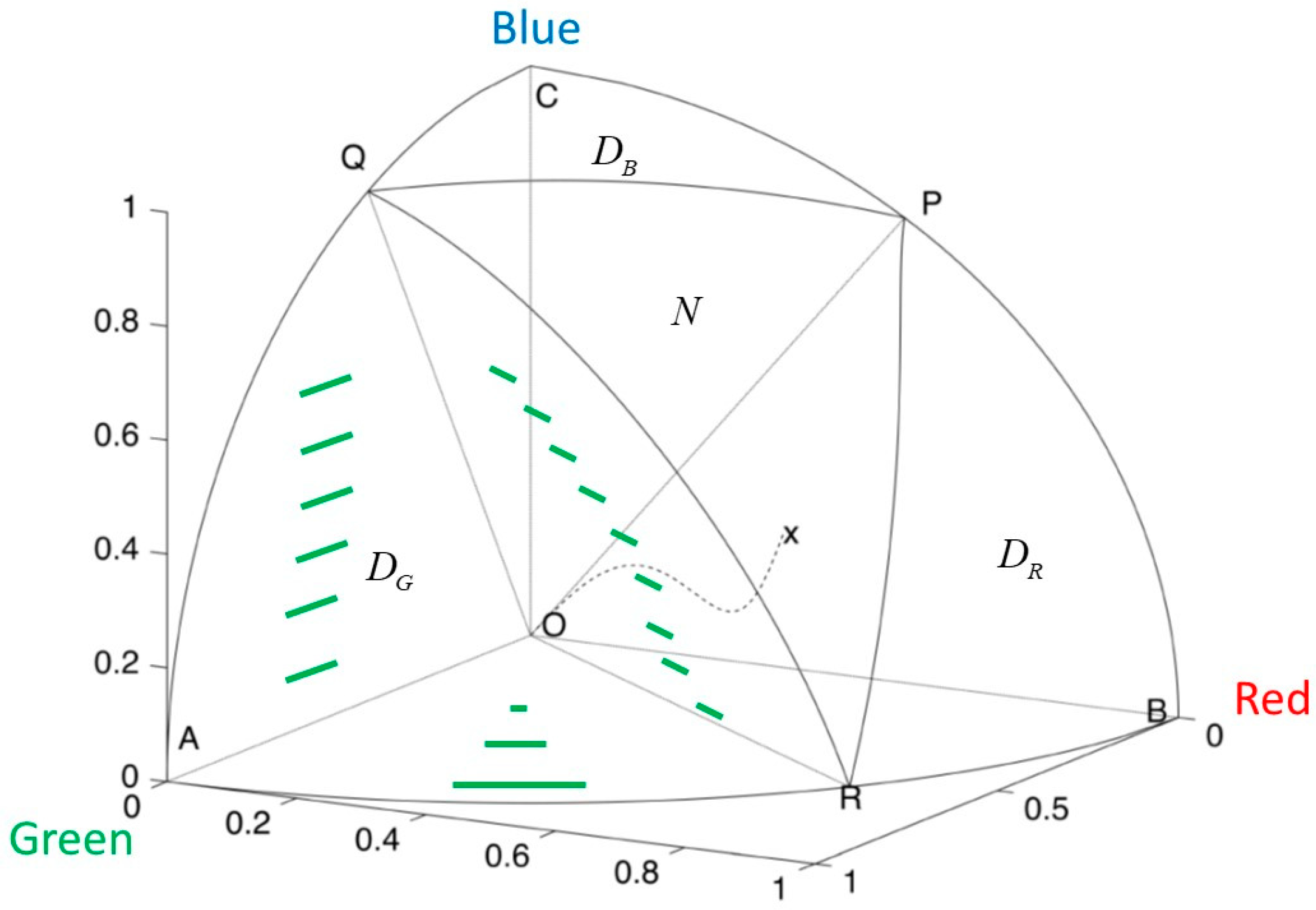
The condition in Equation (28), when applied to each player, divides the non-negative quadrant into four disjoint regions such that player i is dominant in region , i = Blue, Red, Green, and the complement region N is the non-dominant region in which no player is dominant (see Figure 4). For example, OAQR marks the region where Green is dominant. The surface OQR separates Green’s dominant region from N. Similarly, OQP and ORP separate and from N, respectively. The initial states on the line OQ are where and are such that the duel between Blue and Green heads for mutual annihilation.
If a state belongs to a dominant region, then the corresponding dominant player will use the optimal strategy, described at the end of Section 3 for the battle formalized in Equation (10), to guarantee a win. As for an initial state in region N, it is shown in [25] that for each such state there exists a fire-allocation that leads to mutual annihilation. It is always possible, and fairly easy, to find fire strategies that do not shift the current balance of power, by keeping the ratios and fixed throughout. If all players adopt such a strategy, then the resulting force trajectory is a straight line from x in Figure 4 toward (0,0,0). If some player tries to outwit the other players and divert from the status quo, then the relative force sizes may change over time, but such attempts are futile. Defining an appropriate n-person nonzero-sum game and using Nash equilibria, it is shown that such a curve must end up at the origin (see the dotted curve in Figure 4).
In conclusion, the insight from multilateral Lanchester conflicts is clear: either a single player is strong enough to beat all other opponents combined, or all players are destined to a prolonged attritional stalemate that culminates in mutual annihilation. The prolonged war in Syria is an example of such dynamics. Only the appearance of a dominant player (e.g., Russia) can end it with a victory.
7. Summary
Lanchester models of warfare have been around for over a century. They have played a major role in modeling and analyzing regular force-on-force engagements, in particular battles during WWII. Recent conflict situations are not regular in the sense that they are profoundly asymmetric, they increasingly rely on data and information, they are affected by the behavior of civilians and they may involve more than two adversaries.
In this paper, we reviewed recent advances in modeling the aforementioned features of modern combat situations in the context of Lanchester theory. We described some important insights regarding the fate of these situations, as obtained from implementing such models. The main takeaways are: (a) guerrilla forces have an inherent advantage over state forces because the latter suffer from reduced level of situational awareness and are reluctant to massively hurt civilians among which guerrillas hide, (b) as a consequence of (a), the state forces cannot eradicate an insurgency unless it completely ignores civilian casualties, (c) in a situation of multiple adversaries, the state forces have an optimal target allocation plan that depends on the effectiveness of the state forces and the vulnerability of the adversaries, (d) in multilateral conflicts, either there exists a clear victorious player who wins the conflict even if all other sides collaborate in a coalition, or all players are dragged into a prolonged conflict with no victor.
Future conflicts and combat situations may include several characteristics that lend themselves to new Lanchester-type modeling. First, “soft kills”, such as electronic and information warfare, will become more prevalent in future conflicts. This type of attrition is profoundly different than the legacy “hard kills” in which attrition is irreversible. Lanchester models accounting for a mix of soft and hard kills can help design policies and analyze the tradeoff between the two ways of projecting and enduring military force. Second, future combat will rely on the increased use of unmanned systems, which may change the battlefield landscape in the absence of human fear of death. “Attrition” will have a somewhat different meaning, and modeling it within a Lanchester framework would be challenging. Finally, the possible use of biological weapons of mass destruction may trigger an epidemic with significant effect on conflict outcomes. Combinations of two dynamic models—Lanchester and epidemic spread models such as SIR—will be needed to study such complex attritional situations.
Funding
This paper received no external funding.
Conflicts of Interest
The author declare no conflict of interest.
References
- Washburn, A.; Kress, M. Combat Modeling; Springer: New York, NY, USA, 2009. [Google Scholar]
- Kress, M. Modeling armed conflicts. Science 2012, 336, 865–869. [Google Scholar] [CrossRef] [PubMed] [Green Version]
- Lanchester, F.W. Aircraft in Warfare: The Dawn of the Fourth Arm; Constable and Co.: London, UK, 1916. [Google Scholar]
- Brown, G.; Washburn, A. The Fast Theater Model (FATHM). Mil. Oper. Res. 2007, 12, 33–45. [Google Scholar] [CrossRef]
- Jones, H.W. COSAGE User’s Manual, Volume1-MainReport. Revision 4; CAA-D-93-1-Rev-4; Center for Army Analyses: Fort Belvoir, VA, USA, 1995.
- Sahni, M.; Das, S.K. Performance of maximum likelihood estimator for fitting Lanchester equations on Kursk Battle data. J. Battlef. Technol. 2015, 18, 23–30. [Google Scholar]
- Lucas, T.W.; Turkes, T. Fitting Lanchester equations to the battles of Kursk and Ardennes. Nav. Res. Logist. 2004, 51, 95–116. [Google Scholar] [CrossRef] [Green Version]
- MacKay, N.J.; Price, C.; Wood, A.J. Weight of Shell Must Tell: A Lanchestrian reappraisal of the Battle of Jutland. History 2016, 101, 536–563. [Google Scholar] [CrossRef] [Green Version]
- Keane, T. Combat modelling with partial differential equations. Appl. Math. Model. 2011, 35, 2723–2735. [Google Scholar] [CrossRef] [Green Version]
- Kim, D.; Moon, H.; Park, D.; Shin, H. An efficient approximate solution for stochastic. J. Oper. Res. Soc. 2017, 68, 1470–1481. [Google Scholar] [CrossRef]
- Eldrige, S.A.; Mesterton-Gibbons, M. Lanchester’s attrition models and fights among social animals. Behav. Ecol. 2003, 14, 719–723. [Google Scholar]
- Johnson, D.D.P.; MacKay, N.J. Fight the Power: Lanchester’s laws of combat in human evolution. Evol. Hum. Behav. 2013, 36, 152–163. [Google Scholar] [CrossRef]
- Jorgensen, S.; Sigue, S. A Lanchester-Type Dynamic Game of Advertising and Pricing. In Games in Management Science; Sigue, P.-O., Taboubi, S., Pineau, S., Eds.; Springer: New York, NY, USA, 2020; pp. 1–14. [Google Scholar]
- Stanescu, M.; Barriga, N.; Buro, M. Using Lanchester Attrition Laws for Combat Prediction in StarCraft. In Proceedings of the Eleventh AAAI Conference on Artificial Intelligence and Interactive Digital Entertainment (AIIDE-15), Santa Cruz, CA, USA, 14–18 November 2015; pp. 86–92. [Google Scholar]
- Deitchman, S. A Lanchester model of guerrilla war. Oper. Res. 1962, 10, 818–827. [Google Scholar] [CrossRef]
- Helmbold, R.; Rehm, A. Translation of “The Influence of the Numerical Strength of Engaged Forces in Their Casualties”. In Naval Research Logistics; Osipov, M., Ed.; Wiley: Hoboken, NJ, USA, 1995; Volume 42, pp. 435–490. [Google Scholar]
- Taylor, J. Lanchester Models of Warfare; INFORMS: Rockville, MD, USA, 1983. [Google Scholar]
- Schaffer, M.B. Lanchester models of Guerrillla engagements. Oper. Res. 1968, 16, 457–488. [Google Scholar] [CrossRef] [Green Version]
- Gabriel, R.A. Lessons of war: The IDF in Lebanon. Mil. Rev. 1984, 64, 47–65. [Google Scholar]
- Lin, K.Y.; MacKay, N.J. The optimal policy for the one-against-many heterogeneous lanchester model. Oper. Res. Lett. 2014, 42, 473–477. [Google Scholar] [CrossRef]
- Kress, M.; MacKay, N. Bits or Shots in Combat? The Generalized Deitchman Model of Guerrilla Warfare. Oper. Res. Lett. 2014, 42, 102–108. [Google Scholar] [CrossRef]
- Kaplan, E.; Kress, M.; Szechtman, R. Confronting Entrenched Insurgents. Oper. Res. 2010, 58, 329–341. [Google Scholar] [CrossRef] [Green Version]
- Kress, M.; Szechtman, R. Why Defeating Insurgencies is Hard: The Effect of Intelligence in Counterinsurgency Operations—A Best Case Scenario. Oper. Res. 2009, 57, 578–585. [Google Scholar] [CrossRef] [Green Version]
- Kress, M.; Caulkins, J.P.; Feichtinger, G.; Grass, D.; Seidl, A. Lanchester model for three-way combat. Eur. J. Oper. Res. 2018, 264, 46–54. [Google Scholar] [CrossRef]
- Kress, M.; Lin, K.; MacKay, N. The Attrition Dynamics of Multilateral War. Oper. Res. 2018, 66, 950–956. [Google Scholar] [CrossRef]
- Kilgour, D.M.; Brams, S.J. The truel. Math. Mag. 1997, 70, 315. [Google Scholar] [CrossRef]
Figure 1.
The function and the regions in which state forces and insurgents increase or decrease.
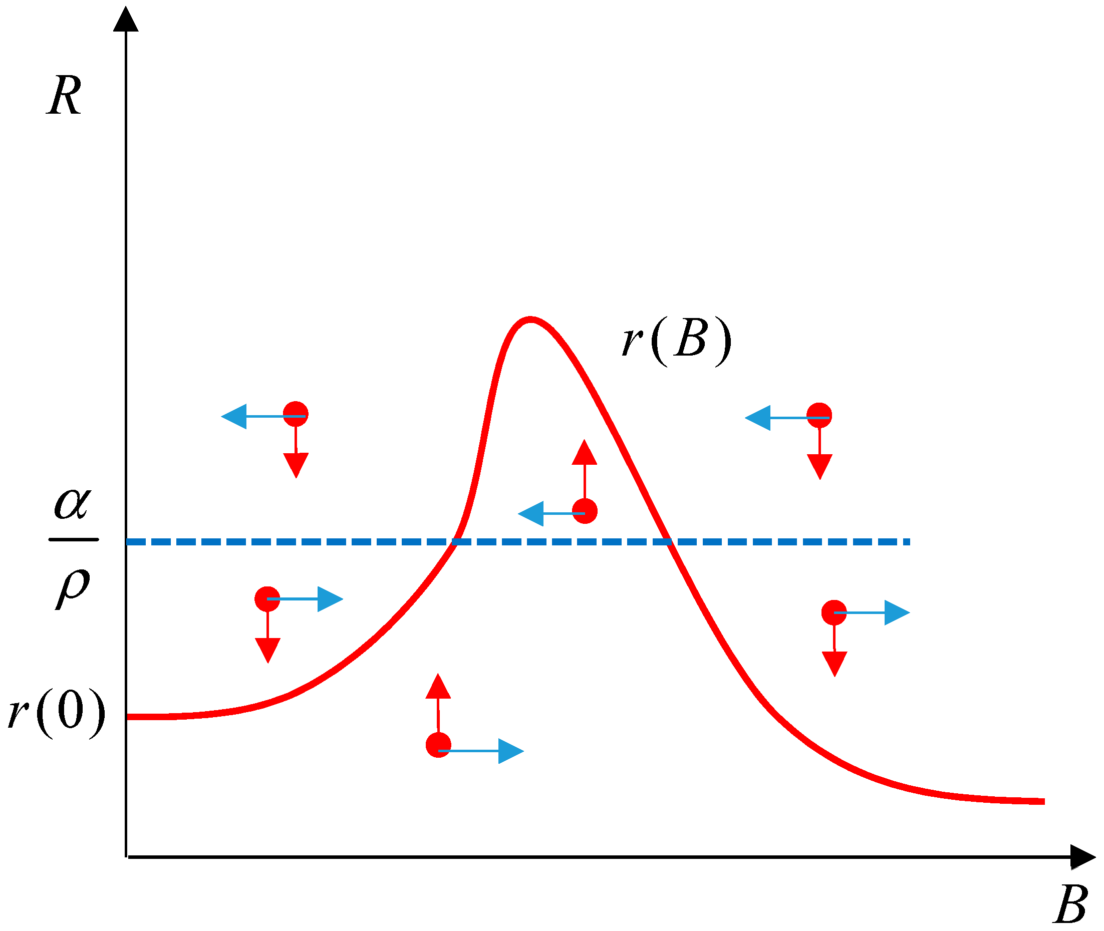
Figure 2.
Winning regions. The solid curves represent points of mutual annihilation at the second stage by the two adjacent players, while the dotted lines indicate points of mutual annihilation at the first stage.
Figure 2.
Winning regions. The solid curves represent points of mutual annihilation at the second stage by the two adjacent players, while the dotted lines indicate points of mutual annihilation at the first stage.
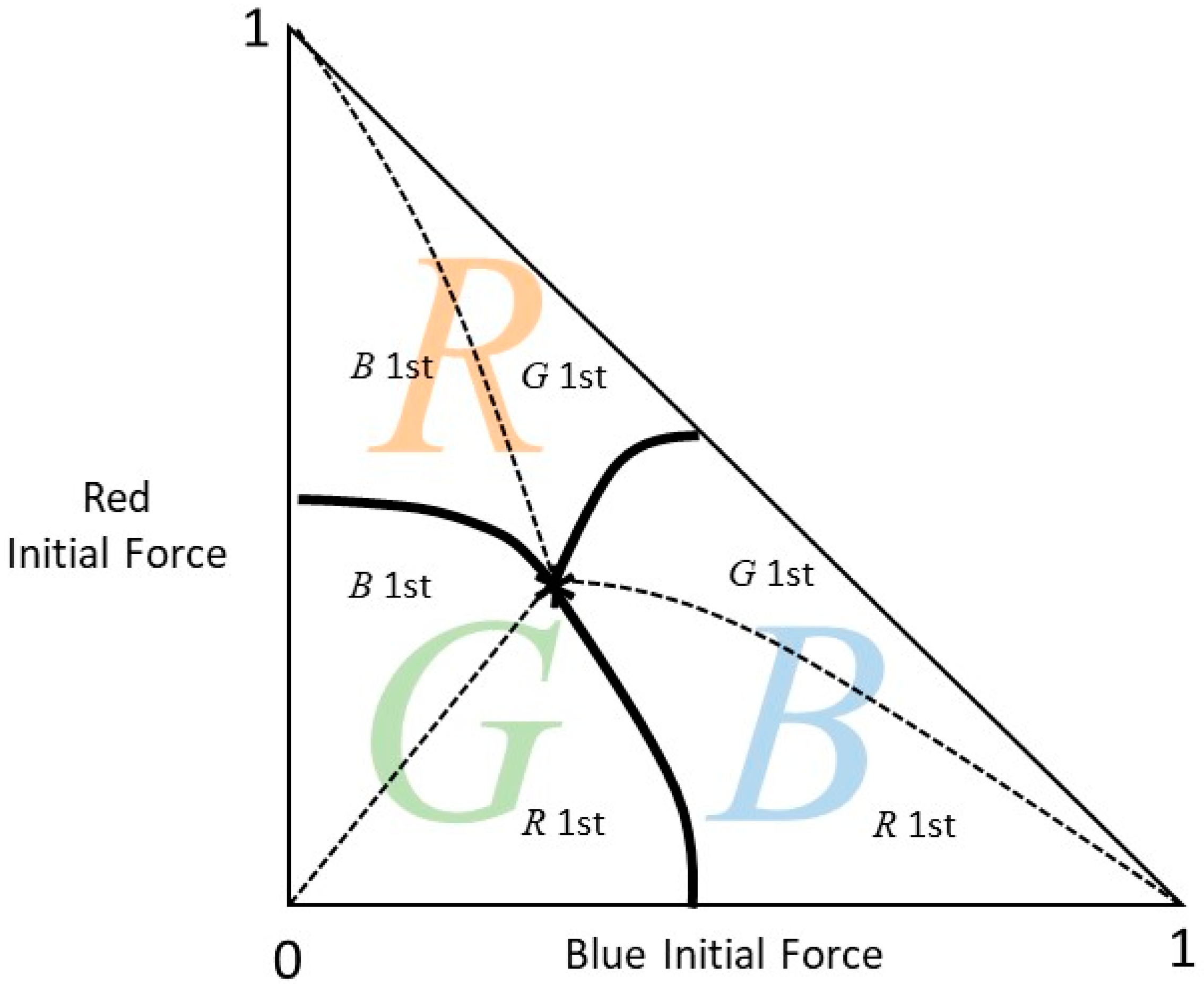
Figure 3.
Unconditional winning regions, optimized winning region, and “victor maker” region for the case where the main battle is between Blue and Green.
Figure 3.
Unconditional winning regions, optimized winning region, and “victor maker” region for the case where the main battle is between Blue and Green.
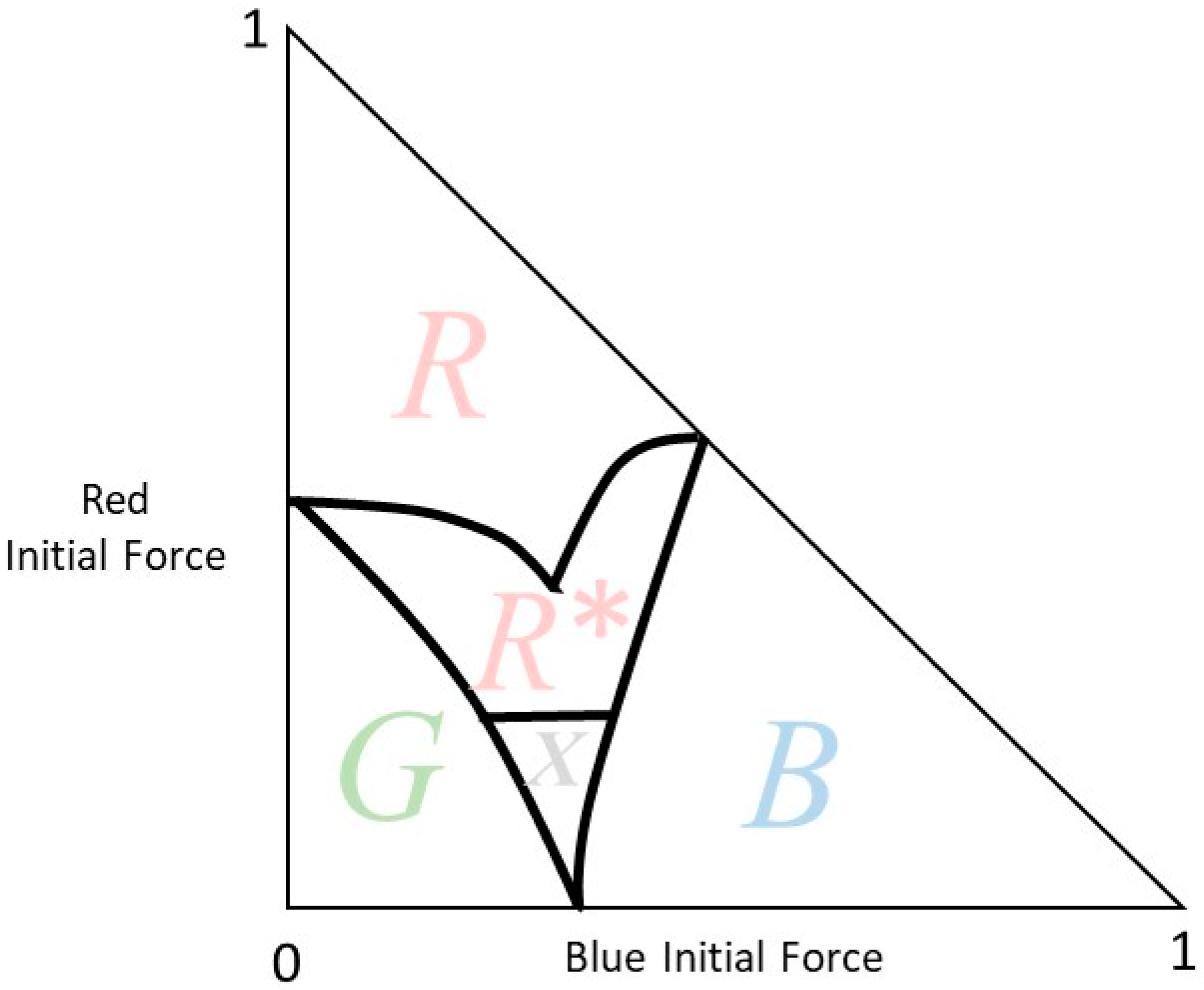
Figure 4.
The case of players where x marks initial force relative sizes and the dashed trajectory indicates the path to mutual annihilation.
Figure 4.
The case of players where x marks initial force relative sizes and the dashed trajectory indicates the path to mutual annihilation.
© 2020 by the author. Licensee MDPI, Basel, Switzerland. This article is an open access article distributed under the terms and conditions of the Creative Commons Attribution (CC BY) license (http://creativecommons.org/licenses/by/4.0/).
Share and Cite
MDPI and ACS Style
Kress, M. Lanchester Models for Irregular Warfare. Mathematics 2020, 8, 737. https://doi.org/10.3390/math8050737
AMA Style
Kress M. Lanchester Models for Irregular Warfare. Mathematics. 2020; 8(5):737. https://doi.org/10.3390/math8050737
Chicago/Turabian StyleKress, Moshe. 2020. "Lanchester Models for Irregular Warfare" Mathematics 8, no. 5: 737. https://doi.org/10.3390/math8050737
Note that from the first issue of 2016, this journal uses article numbers instead of page numbers. See further details here.