The Generalized Neutrosophic Cubic Aggregation Operators and Their Application to Multi-Expert Decision-Making Method


Abstract
1. Introduction
- -
- First neutrosophic cubic generalized unified aggregation operators are proposed.
- -
- Second neutrosophic cubic quasi-generalized unified aggregation operators are proposed.
- -
- The multi-expert decision-making method is proposed.
- -
- The method is furnished upon numeric data of EMU European Monitory union as an application.
- -
- Comparison is given between some aggregation operators.
2. Preliminaries
3. The Neutrosophic Cubic Generalized Unified Aggregation Operator
Families of NCGUA Operators
- If and for all j, the aggregation operator is deduced to NCUA.
- If and for all j, the aggregation operator is deduced to NCUG.
- If and for all j, the aggregation operator is deduced to NCUQA.
- If and for all j, the aggregation operator is deduced to NCGUG.
- If and for all j, the aggregation operator is deduced to NCQUQA.
4. Neutrosophic Cubic Quasi-Generalized Unified Aggregation Operators
5. The Application of NCQGUA and NCGUA Operators to Multi-Expert Decision-Making Method
5.1. Algorithm
- ➢
- Construction of expert’s criteria matrices for each criterion corresponding to the given alternatives and finite state of nature.
- ➢
- Transformation of expert criteria matrices to general group expert’s matrix by aggregation operator.
- ➢
- Transformation of all the general group experts’ matrices to a single matrix by aggregation operator.
- ➢
- Ranking of alternatives.
5.2. Model Formulation
- Criteria
- Internal economic condition.
- Global economic condition.
- Alternative
- Increase the rates 1%.
- Increase the rates 0.5%.
- No change in rates.
- Decrease the rates 0.5%.
- Decrease the rates 1%.
- State of nature
- Negative growth.
- Growth close to 0.
- Positive growth.
6. Discussion
7. Conclusions
Author Contributions
Funding
Conflicts of Interest
References
- Zadeh, L.A. Fuzzy sets. Inform. Control 1965, 8, 338–353. [Google Scholar] [CrossRef]
- Zadeh, L.A. Outline of a new approach to the analysis of complex system and decision processes interval-valued fuzzy sets. IEEE Trans. 1973, 1, 28–44. [Google Scholar]
- Turksen, I.B. Interval-valued strict preference with Zadeh triples. Fuzzy Sets Syst. 1996, 78, 183–195. [Google Scholar] [CrossRef]
- Atanassov, K.; Gargov, G. Interval-valued intuitionistic fuzzy sets. Fuzzy Sets Syst. 1989, 31, 343–349. [Google Scholar] [CrossRef]
- Atanassov, K. Intuitionistic fuzzy sets. Fuzzy Sets Syst. 1986, 20, 87–96. [Google Scholar] [CrossRef]
- Jun, Y.B.; Kim, C.S.; Yang, K.O. Cubic sets. Ann. Fuzzy Math. Inform. 2012, 1, 83–98. [Google Scholar]
- Garg, H.; Singh, S. A novel triangular interval type-2 intuitionistic fuzzy sets and their aggregation operators. Iran. J. Fuzzy Syst. 2018, 15, 69–93. [Google Scholar]
- Kumar, K.; Garg, H. TOPSIS method based on the connection number of set pair analysis under interval-valued intuitionistic fuzzy set environment. Comput. Appl. Math. 2018, 37, 1319–1329. [Google Scholar] [CrossRef]
- Kaur, G.; Garg, H. Cubic intuitionistic fuzzy aggregation operators. Int. J. Uncertain. Quantif. 2018, 8, 405–427. [Google Scholar] [CrossRef]
- Rani, D.; Garg, H. Distance measures between the complex intuitionistic fuzzy sets and its applications to the decision—Making process. Int. J. Uncertain. Quantif. 2007, 7, 423–439. [Google Scholar] [CrossRef]
- Xu, Z.S. Intuitionistic fuzzy aggregation operators. IEEE Trans. Fuzzy Syst. 2007, 15, 1179–1187. [Google Scholar]
- Xu, Z.S.; Yager, R.R. Some geometric aggregation operators based on intuitionistic fuzzy sets. Int. J. Gen. Syst. 2006, 35, 417–433. [Google Scholar] [CrossRef]
- Smarandache, F. A Unifying Field in Logics: Neutrosophic Logic. Neutrosophy, Neutrosophic Set, Neutrosophic Probability; American Research Press: Rehoboth, NM, USA, 1999. [Google Scholar]
- Smarandache, F. Neutrosophic Set—A Generalization of the Intuitionistic Fuzzy Set. In Proceedings of the IEEE International Conference on Granular Computing, Atlanta, GA, USA, 10–12 May 2006. [Google Scholar]
- Wang, H.; Smarandache, F.; Zhang, Y.Q.; Sunderraman, R. Single valued neutrosophic sets. Multispace Multistruct. 2010, 4, 410–413. [Google Scholar]
- Wang, H.; Smarandache, F.; Zhang, Y.Q. Interval Neutrosophic Sets and Logic: Theory Applications Computing; Hexis: Phoenix, AZ, USA, 2005. [Google Scholar]
- Jun, Y.B.; Smarandache, F.; Kim, C.S. Neutrosophic cubic sets. New Math. Nat. Comput. 2015, 8, 41. [Google Scholar] [CrossRef]
- Liu, P.; Wang, Y. Multiple attribute decision-making method based on single-valued neutrosophic normalized weighted bonferroni mean. Neural Comput. Appl. 2014, 25, 2001–2010. [Google Scholar] [CrossRef]
- Abdel-Basset, M.; Zhou, Y.; Mohamed, M.; Chang, V. A group decision making framework based on neutrosophic vikor approach for e-government website evaluation. J. Intell. Fuzzy Syst. 2018, 34, 4213–4224. [Google Scholar] [CrossRef]
- Nancy, G.H.; Garg, H. Novel single-valued neutrosophic decision making operators under frank norm operations and its application. Int. J. Uncertain. Quantif. 2014, 6, 361–375. [Google Scholar] [CrossRef]
- Peng, X.D.; Dai, J.G. A bibliometric analysis of neutrosophic set: Two decades review from 1998–2017. Artif. Intell. Rev. 2018. [Google Scholar] [CrossRef]
- Li, B.; Wang, J.; Yang, L.; Li, X. A novel generalized simplified neutrosophic number Einstein aggregation operator. Int. J. Appl. Math. 2018, 48, 67–72. [Google Scholar]
- Biswas, P.; Pramanik, S.; Giri, B.C. Topsis method for multi-attribute group decision-making under single-valued neutrosophic environment. Neural Comput. Appl. 2016, 27, 727–737. [Google Scholar] [CrossRef]
- Ye, J. Exponential operations and aggregation operators of interval neutrosophic sets and their decision making methods. SpringerPlus 2016, 5, 1488. [Google Scholar] [CrossRef]
- Garg, H.; Nancy, G. Multi-criteria decision-making method based on prioritized muirhead mean aggregation operator under neutrosophic set environment. Symmetry 2018, 10, 280. [Google Scholar] [CrossRef]
- Garg, H.; Nancy, B. Some hybrid weighted aggregation operators under neutrosophic set environment and their applications to multicriteria decision-making. Appl. Intell. 2018, 1–18. [Google Scholar] [CrossRef]
- Jha, S.; Kumar, R.; Chatterjee, J.M.; Khari, M.; Yadav, N.; Smarandache, F. Neutrosophic soft set decision making for stock trending analysis. Evol. Syst. 2019, 1–7. [Google Scholar] [CrossRef]
- Khan, M.; Gulistan, M.; Khan, M.; Smaradache, F. Neutrosophic cubic Einstein geometric aggregatio operatorswith application to multi-creiteria decision making theory method. Symmetry 2019, 11, 247. [Google Scholar]
- Zhan, J.; Khan, M.; Gulistan, M.; Ali, A. Applications of neutrosophic cubic sets in multi-criteria decision making. Int. J. Uncertain. Quantif. 2017, 7, 377–394. [Google Scholar] [CrossRef]
- Banerjee, D.; Giri, B.C.; Pramanik, S.; Smarandache, F. GRA for multi attribute decision making in neutrosophic cubic set environment. Neutrosophic Sets Syst. 2017, 15, 64–73. [Google Scholar]
- Lu, Z.; Ye, J. Cosine measure for neutrosophic cubic sets for multiple attribte decision making. Symmetry 2017, 10, 121–131. [Google Scholar]
- Pramanik, S.; Dalapati, S.; Alam, S.; Roy, S.; Smarandache, F. Neutrosophic cubic MCGDM method based on similarity measure. Neutrosophic Sets Syst. 2017, 16, 44–56. [Google Scholar]
- Shi, L.; Ye, J. Dombi aggregation operators of neutrosophic cubic set for multiple attribute deicision making. Algorithms 2018, 11, 29. [Google Scholar] [CrossRef]
- Ye, J. Operations and aggregation methods of neutrosophic cubic numbers for multiple attribute decision-making. Soft Comput. 2018, 22, 7435–7444. [Google Scholar] [CrossRef]
- Alhazaymeh, K.; Gulistan, M.; Khan, M.; Kadry, S. Neutrosophic cubic Einstein hybrid geometric aggregation operators with application in prioritization using multiple attribute decision-making method. Mathematics 2019, 7, 346. [Google Scholar]
- Figueira, J.; Greco, S.; Ehrgott, M. Multiple Criteria Decision Analysis: State of the Art Surveys; Springer: Boston, MA, USA, 2005. [Google Scholar]
- Zavadskas, E.K.; Turskis, Z. Multiple criteria decision making (MCDM) methods: An overview. Technol. Econ. Dev. Econ. 2011, 17, 397–427. [Google Scholar] [CrossRef]
- Zhou, L.G.; Wu, J.X.; Chen, H.Y. Linguistic continuous ordered weighted distance measure and its application to multiple attributes group decision making. Appl. Soft Comput. 2014, 25, 266–276. [Google Scholar] [CrossRef]
- Merigó, J.M.; Gil-Lafuente, A.M.; Yu, D.; Llopis-Albert, C. Fuzzy decision making in complex frameworks with generalized aggregation operators. Appl. Soft Comput. 2018. [Google Scholar] [CrossRef]


| Min | Min | Min | Max | |
| Min | NCUGA | Max | ||
| Min | NCUGA | max | ||
| Min | NCUGA | Max | ||
| Min | NCUGA | Max |
| NCAO Operator | ||
|---|---|---|
| NCQA operator | ||
| NCHA operator | ||
| NCCA operator | ||
| NCGA operator | ||
| NCAUAQA operator | ||
| NCHUHA operator | ||
| NCUCA operator | ||
| NCUGA operator |
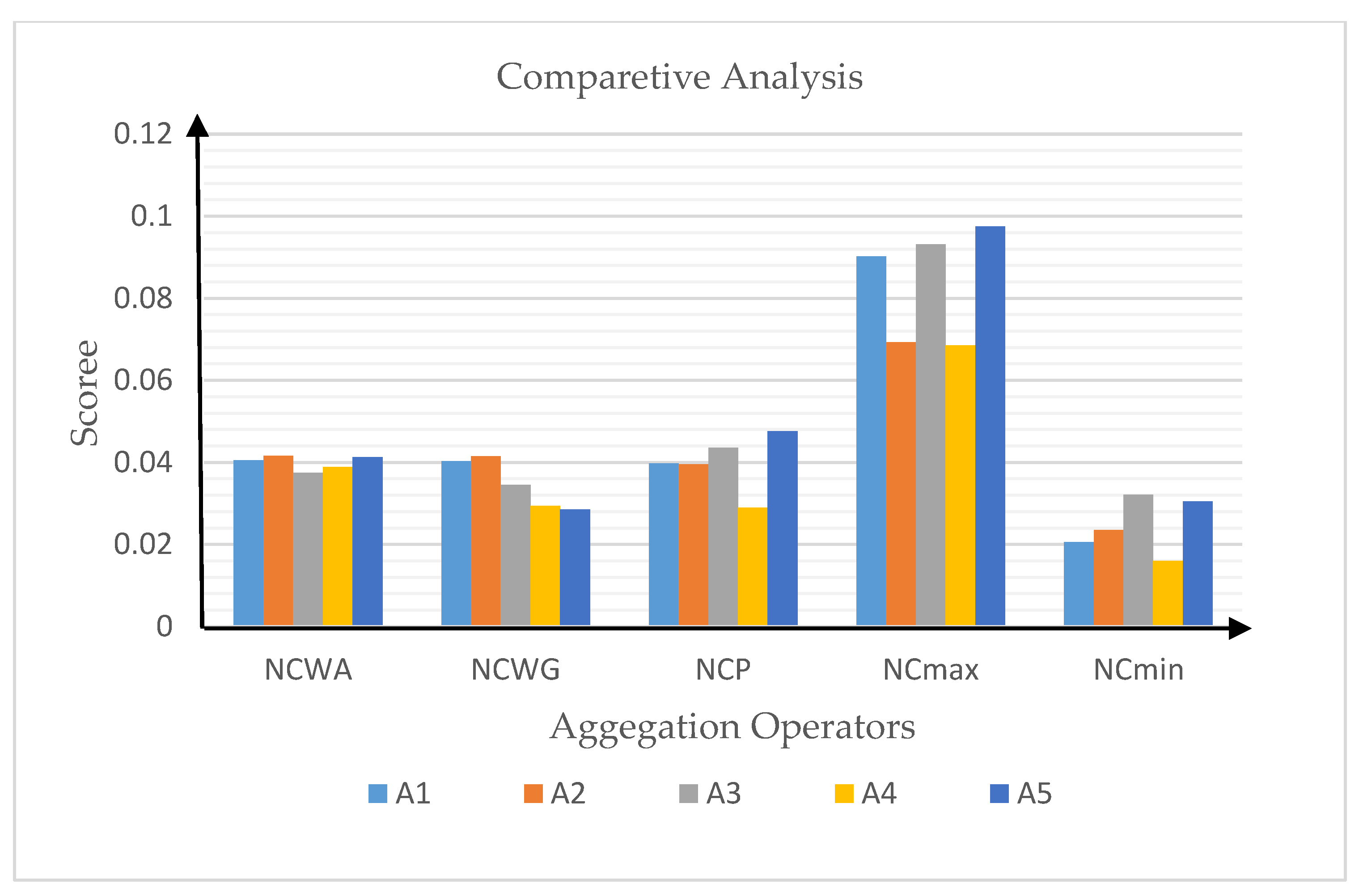
| Operators | Ranking |
|---|---|
| NCWA | |
| NCWG | |
| NCP | |
| NCmax | |
| NCmin |
| Operators | Ranking |
|---|---|
| FWA | |
| FOWA | |
| FPA | |
| FMax | |
| FMin |
© 2020 by the authors. Licensee MDPI, Basel, Switzerland. This article is an open access article distributed under the terms and conditions of the Creative Commons Attribution (CC BY) license (http://creativecommons.org/licenses/by/4.0/).
Share and Cite
Khan, M.; Gulistan, M.; Ali, M.; Chammam, W. The Generalized Neutrosophic Cubic Aggregation Operators and Their Application to Multi-Expert Decision-Making Method. Symmetry 2020, 12, 496. https://doi.org/10.3390/sym12040496
Khan M, Gulistan M, Ali M, Chammam W. The Generalized Neutrosophic Cubic Aggregation Operators and Their Application to Multi-Expert Decision-Making Method. Symmetry. 2020; 12(4):496. https://doi.org/10.3390/sym12040496
Chicago/Turabian StyleKhan, Majid, Muhammad Gulistan, Mumtaz Ali, and Wathek Chammam. 2020. "The Generalized Neutrosophic Cubic Aggregation Operators and Their Application to Multi-Expert Decision-Making Method" Symmetry 12, no. 4: 496. https://doi.org/10.3390/sym12040496
APA StyleKhan, M., Gulistan, M., Ali, M., & Chammam, W. (2020). The Generalized Neutrosophic Cubic Aggregation Operators and Their Application to Multi-Expert Decision-Making Method. Symmetry, 12(4), 496. https://doi.org/10.3390/sym12040496