Lifetime Expectancy of Li-Ion Batteries used for Residential Solar Storage

Abstract

This paper analyses the degradation that is experienced by different types of Li-ion batteries when used as home solar storage systems controlled to minimize the electricity bill of the corresponding household. Simulating the annual operation of photovoltaic (PV) residential systems with batteries at different locations was undertaken to perform the study and it uses actual consumption values and real PV production profiles, as well as validated semi-empirical ageing models of the batteries. Therefore, the work provides a realistic prognosis around the lifetime expectancies for the different Li-ion chemistries.

1. Introduction

PV technology has become the most important power generation source worldwide in terms of added capacity per year since 2016, overtaking wind power, which was the leading technology up to then [1]. In all, new PV installations represented approximately 100 GW in 2018, achieving an accumulated capacity that goes beyond 500 GW [2]. This evolution has been possible thanks to the huge price decrease experienced by this industry due to the economies of scale in the last decade. In accordance, the cost for residential grid-connected PV systems has worldwide-averaged dropped down to around 1.28 €/W, being approximately 20% higher than in Europe, where 1.13 €/W can be generally found, and 30% higher than in Australia, where prices plummeted to 0.95 €/W [3]. Thanks to it, the residential market has also experienced a big deployment of PV installations mainly envisaged for self-generation, which achieves very high shares of the energy production-consumption in certain local low voltage grids (Figure 1).

However, large amounts of behind-the-meter solar installations that produce stochastically intermittent energy can imply stability problems at the low voltage grid level [4]. Hence, new technical and regulatory solutions have to be implemented to avoid running into the problem of systematically having to curtail part of their production. The introduction of energy storage (ES) systems, usually batteries, within the households [5,6,7]. Batteries for energy storage in buildings have been around for a long time in both stand-alone (off-grid) and commercial back-up power systems (UPS). However, even with the still relatively high cost of batteries, their combined use with solar systems has also started to gain momentum over the last few years. This is because such systems not only allow for reducing the intermittency of the local production, stabilizing the low voltage grid, but also make it possible to optimize the energy bill for the installation owners and even provide extended supply security, which cannot be taken for granted everywhere. In this way, some specialized consultants indicate that out of the 4 GW of batteries with an 8 GWh capacity to be deployed globally in 2019 (with calculations to achieve 15 GW with a 44 GWh capacity in 2024 and between 180 and 420 GWh in 2030), more than half could be distributed [8], i.e., behind the meter PV residential systems with batteries, also known as home solar storage systems. Among them, these are clearly set to spread across Europe. Italy seems, in this sense, to be consolidating its position as the second-largest market after Germany and Spain is well positioned to develop its own sizable market, although this is always very dependent on the changing political framework of the country. France and the United Kingdom keep being promising markets, although they have not clearly emerged yet [9]. Beyond Europe, the USA is a consolidated market, mainly in states, such as California, and also Australia is starting to take off. Note how, in the latter, there is great incentive to store solar energy as the solar feed-in tariff has been lately reduced to as little as 5 ¢ per kWh (¢—cent), while the cost to purchase electricity is closer to 30 ¢ per kWh. This has become a driving force and great incentive to store solar energy, rather than send it to the power grid for little return.

As can be understood in such a context, a great bunch of behind the meter PV residential systems with batteries are commercially available [10] and they have been largely discussed and analyzed in the literature. However, most of the previous academic works are focused on optimizations that are related to the sizing of the battery system [11,12,13] or to maximizing the economic income of the PV installations [14,15,16,17]. However, few among the previous works have already taken the degradation of the batteries during the lifespan of the system into account. Degradation evolution is very important for the economic analysis of these systems, which are still costly, as already indicated, and whose profitability is still under discussion [18]. In fact, degradation is already a key parameter in the profitability analyses of batteries being proposed in applications, such as ramp rate control of large renewable power generation plants [19,20], ancillary services [21,22], energy arbitrage, and peak shaving provided by large energy storage systems [23,24], and even for electric vehicle integration [25]. Among those published for the residential solar storage sector, some can be highlighted. For instance, the authors in [26] analyze the impact of the internal battery pack circuit design on the system operation and its corresponding degradation. Another approach is proposed in [27] and in [28], in which forecasting methodologies are included to optimize the operation of the system with the aim to enhance the battery lifetime. Finally, an economic optimization of the batteries sizing taking into account the ageing of the batteries is performed in [29]. However, they use either simplified battery degradation models [27,28] or generic ones that they adapt to different types of batteries being valid, even for lead acid models [29].

This work assumes that the sizing and control of the system is a mature domain nowadays and it focuses on the analysis of degradation that the different Li-ion batteries used in such an application would experience under a wide range of operational conditions. The analysis is based on well-known accepted detailed degradation models for the specific chemistries under discussion, which have also been adapted here to actual state-of-the-art commercial battery packs, which allows for providing accurate and realistic lifetime expectancies for those particular chemistries included in current commercial products. Therefore, the results of this work are a valuable reference for analyzing the profitability of these storage solutions.

The structure of this paper is as follows. Section 2 is devoted to the definition of Li-ion chemistries to be used in residential PV storage, to the introduction of their corresponding degradation models, and to describe the mode of operation of the batteries that are designed to minimize the operational cost of the system. Subsequently, Section 3 summarizes the degradation results experienced by the batteries according to one year long simulations that were performed while using MATLAB^® (Natick, MA, USA) and the discussion on the expected lifetime estimations. Finally, some concluding remarks are introduced.

2. Methods

The combined use of Li-ion batteries with solar PV systems is gaining momentum, because such systems not only allow reducing the intermittency of the local production, but also provide a boost in the handling of local solar generation $\left(P_{PV}\right)$, i.e., increasing the amount of self-production that becomes self-consumed [30]. Moreover, solar storage systems make it possible to optimize the energy bill for the installation owners by peak shaving [5,24] or by profiting a time-of-use electricity rate structure for energy arbitrage [31,32]. This is, as coupled with solar, battery systems can store the excess generation and allow the customer to dispatch the stored energy during peak load hours when electricity is more expensive. In the coming future (already a reality in the so-called Virtual Power Plants, VPP) additional revenues can be passed onto the battery users when the system is centrally controlled by the VPP operator and the energy that is stored in the batteries is accordingly dispatched to provide grid support for homeowners that are interested in sharing the resource with the utility.

Nonetheless, among the different potential applications that are defined for home storage systems, these are mainly installed nowadays for energy arbitrage and peak shaving (also back-up service in certain locations such as California). Therefore, this work analyzes the lifetime expectancy that is associated with two different Li-ion chemistries when used under such control strategy. To do so, the different Li-ion chemistries are reviewed in the following and some are highlighted. The various degradation models used in the analysis are then introduced. Finally, the optimization introduced controlling the operation of the home solar storage system is presented. The operation of different home storage systems, in terms of power and energy ratings, will be then simulated in an annual context at different locations (radiation patterns) and within different households (load patterns).

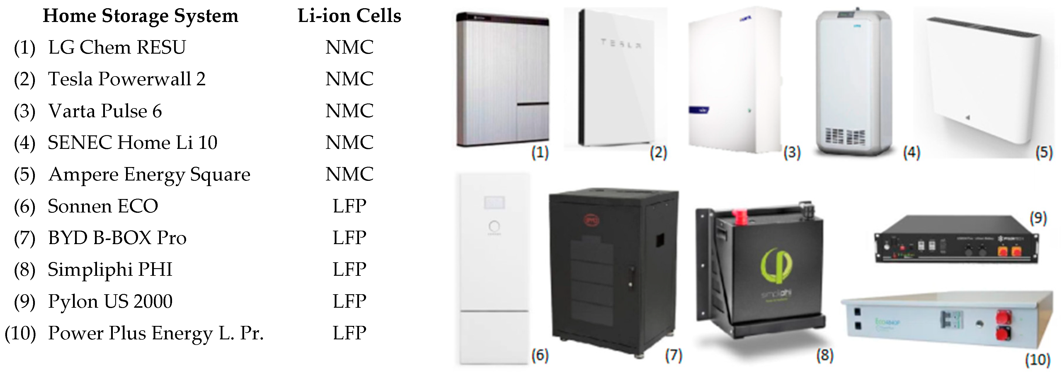
2.1. Li-ion Batteries and their Degradation Models

Nowadays, the generic label Li-ion batteries cover up to six different battery chemistries while using some type of lithium alloy in their electrodes. These correspond to: Lithium Cobalt Oxide (LiCoO₂), Lithium Manganese Oxide (LiMn₂O₄), Lithium Iron Phosphate (LiFePO₄), Lithium Nickel Cobalt Aluminum Oxide (LiNiCoAlO2), Lithium Nickel Manganese Cobalt Oxide (LiNiMn-CoO₂), and Lithium Titanate (Li4Ti5O12). The various Li-ion families present different properties and characteristics as a function of their internal structure and composition [33], which involve varying capabilities in terms of specific power (W/kg), specific energy (Wh/kg), thermal stability, cyclability, and performance. They also differ in cost and lifetime expectancy.

Depending on the application and the associated battery requirements, a different chemistry will be of choice. For home storage applications, where batteries have been defined to be mainly used to maximize the PV production exploitation while reducing the economic cost of the electricity consumption in the household via energy arbitrage or peak shaving, safety, and space limitations are generally assumed to be the most defining or limiting parameters. In this context, LiFePO₄ (LFP) and LiNiMn-CoO₂ (NMC) cells constitute the batteries best fitting these constraints, which can be confirmed by analyzing the different models commercially available nowadays, as in Figure 2.

Among them, although LFP batteries have been traditionally more expensive than the NMC ones, now prices have matched. Therefore, vendors are looking favorably at them due to their lack of Cobalt as fire safety regulations become stricter, even though energy density is a drawback for LFP. Attending to the different considerations introduced, the degradation and the lifetime expectancy for these two chemistries are analyzed in this work. In this sense, although different types of models for predicting the lifetime expectancies are available in the literature [34,35,36,37], semi-empirical models (equations based on real lab measurements) are considered to be the best approach in terms of complexity and reliability tradeoff in this work, as it is usually assumed in studies analyzing the degradation of the Li-ion batteries subject to real operation scenarios [38]. Most of these models take different types of stress factors [34,39,40] that degrade the cells via the so called calendar cycle (associated to temperature and state of charge during stand-by operation) or cycle ageing (also associated to temperature, and to the number, depth of discharge, and average state of charge for the cycles, as well as the C-rate) into account [39,41,42]. Among the different proposals of semi-empirical degradation models, two different models that disregard the C-rate stress factor and focus on the others have been used as reference models. This is due to the fact that most home solar storage systems usually limit via software their power exchange capability to values below 1 C that would be a certain limit beyond which C-rate becomes a significant stress factor [43,44]. These models, together with the corresponding improved models that are updated to state-of-the-art cells for each of the chemistries, are introduced in the following.

2.2. Reference Degradation Model for LiFePO₄ Cells

The semi-empirical degradation analysis proposal used as reference or base model in this work to estimate the lifetime of LFP cells is that suggested by Stroe et al. [45]. This paper, which was published in 2014, proposes a model that was developed for cylindrical battery cells as those from SAFT Batteries, model VL41M [46]. The model analyzes the loss of battery capacity due to both the use of the battery (cycle ageing) and the pass of the time itself (calendar ageing). The value of the capacity reduction (C_fade) that is associated to the latter is defined by:

$$C_{fad{e}_{cal\_LFP}}\left(T,t\right)={\alpha }_{cal\_LFP}\times e^{{\beta }_{cal}\times T}\times t^{0.5}$$

(1)

where ${\alpha }_{cal\_LFP}$ and ${\beta }_{cal}$ are two parameters whose values depend on the precise model of cell being analysed, T is the temperature (in Kelvin), and t is the time (in months). Moreover, the capacity reduction that is associated to the operation (cycling), responds to:

$$C_{fad{e}_{cyc}\_LFP}\left(T,NC\right)={\alpha }_{cyc\_LFP}\times e^{{\beta }_{cyc}\times T}\times N{C}^{0.5}$$

(2)

where ${\alpha }_{cyc\_LFP}$ and ${\beta }_{cyc}$ are again other two parameters whose values depend on the model of cell being analysed, and NC represents the number of equivalent full cycles, which are calculated from the annual evolution of the state of charge (SOC) of the battery registered when operated in a home storage application. This SOC evolution is introduced to the Rainflow Counting Algorithm (RFC) [47], which is capable of grouping those cycles with an equal depth of discharge (DoD) and average SOC. Afterwards, by means of the Palmgren–Miner rule and the capacity evolution curves of the batteries provided by manufacturers, the NC value can be obtained, as summarized in Figure 3.

Once the NC are defined, its value is introduced into Equations (1) and (2) together with the T values and the time range analysed. The resulting C_fade values are combined to finally provide the lifetime estimation prognosis, in years, by means of the following equation:

$$\mathrm{EOL}\%\times C_0=C_{fad{e}_{cal}}\left({\mathrm{year}}_{\mathrm{EOL}},T\right)+C_{fad{\mathrm{e}}_{\mathrm{cyc}}}\left(NC,T\right)\times year{s}_{EOL}$$

(3)

Note how this equation takes into account that battery manufacturers usually define the end-of-life (EOL) of the LFP batteries as the moment when the capacity retained by the cell is equal to a given percentage of its initial capacity (C₀) that, still depending on the cell model, can range from 60% to 80% (70% for the cell under analysis). The solution, in years, to this equation is the estimated lifetime expectancy for the battery.

2.3. Reference Degradation Model for Li(NiMnCo)O₂ Cells

The semi-empirical degradation model used, as reference, analyzing the lifetime of NMC type cells is that proposed by Schmalstieg et al. [48]. Note how, also in this case, the work published in the same year 2014 focuses on the behavior of cylindrical cells. More precisely, it is developed for the Sanyo UR18650E cell [49]. Again, as for the LFP model, the degradation is analyzed as the loss of battery capacity associated to both calendar and cycling. The first of them is described according to:

$$C_{fad{e}_{cal\_NMC}}\left(V,T,t\right)={\alpha }_{cal\_NMC}\times \left(V-3.15\right)\times e^{-\frac{6976}{T}}\times t^{0.75}$$

(4)

where ${\alpha }_{cal\_NMC}$ is a parameter that depends on the model of cell under consideration, V is the average daily voltage (in Volts), T is the temperature (in Kelvin), and t is the time (in days). Conversely, the degradation that is associated to the use of the battery is calculated by:

$$C_{fad{e}_{cyc}}\left(\mathrm{Q},ØV,\Delta DOD\right)={\alpha }_{cyc\_NMC}\times \left(1.8\times {\left(ØV-3.667\right)}^2+\Delta DoD+0.1862\right)\times {\mathrm{Q}}^{0.5}$$

(5)

It can be stated again that ${\alpha }_{cyc\_NMC}$ is a parameter that depends on the model of cell under consideration, Q stands for the charge throughput (in ampere-hour), ∅V is the average voltage for each cycle (in Volts), and ΔDoD is the depth of discharge of the cycle (in range of 0–1). Subsequently, the resulting C_fade values correspondingly associated to calendar and cycle degradation are combined to finally provide the lifetime estimation prognosis ($yea{r}_{EOL}$, in years), by means of:

$$\mathrm{EOL}\%\times C_0=C_{fad{e}_{cal}}\left({\mathrm{year}}_{\mathrm{EOL}},T,V\right)+C_{fad{\mathrm{e}}_{\mathrm{cyc}}}\left(Q,\varnothing V,\Delta DoD\right)\times year{s}_{EOL}$$

(6)

This final equation takes once again into account the EOL of the batteries as a percentage of its C₀, also being estimated at the 70% for this cell, according to manufacturer’s information.

2.4. Degradation Models for State-of-the-Art Cells

As indicated, previous degradation models were published several years ago and they correspond to LFP and NMC cylindrical cells commercialized in the first half of this decade. Li-ion cells have rapidly evolved lately and current commercial models present extended capabilities that provide much improved performances, mainly in terms of life span and warranty. This is due to the improvement in both the current internal design of the cells (most of them evolving towards pouch cells for these applications) and in their arrangement within the battery packs. In this way, new battery packs present better thermal management and reduced internal resistances, which imply lower internal operation temperatures and reduced degradation due to current exchanges.

Among the different commercial models that are available in the market, this work focuses on the solutions belonging to two of the main global energy storage players nowadays: the BYD B-BOX Pro as LFP system and the LG Chem RESU as NMC system. For the case of the first one, BYD comes with one of the best warranties on the market, with an estimated 60% retained capacity after 10 years and up to around 5100 full cycles, if operated in a range of temperatures between −10 °C and 50 °C. This corresponds to an overall 23.9 MWh energy throughput capability for the B-BOX Pro 7.5 [50]. LG Chem, on the other hand, implements NMC pouch cells with an estimated minimum 60% retained capacity after 10 years if being operated within −10 °C and 45 °C and for an overall 20 MWh energy throughput capability for its RESU6.5 battery pack [51], which implies 4000 full cycles.

Therefore, apart from the previously introduced reference degradation models, this work considers other two models that adapt the trending curves defined through Equations (1)–(6) to the warranties that are defined by BYD and LG for their current commercial products, B-BOX and RESU, respectively. In this way, the weighted effect of the different stress factors over the global ageing of the cells demonstrated by previous studies is kept, but it is updated to the current performances of the cells being installed in commercial home storage systems nowadays. These are labelled as State-of-the-art (SoA) models and they have been validated while using on-the-field-data and data provided by sponsors of the study and protected by a Non-Disclosure Agreement (NDA). The corresponding values for the coefficients of the different models are introduced in

Table 1. Calendar and Cycling Aging Models’ Coefficients for the different Battery Types analyzed.

Battery Model	${\mathit{\alpha }}_{\mathit{c}\mathit{a}\mathit{l}\_\mathit{L}\mathit{F}\mathit{P}}$	${\mathit{\alpha }}_{\mathit{c}\mathit{y}\mathit{c}\_\mathit{L}\mathit{F}\mathit{P}}$	${\mathit{\beta }}_{\mathit{c}\mathit{a}\mathit{l}}$	${\mathit{\beta }}_{\mathit{c}\mathit{y}\mathit{c}}$	${\mathit{\alpha }}_{\mathit{c}\mathit{a}\mathit{l}\_\mathit{N}\mathit{M}\mathit{C}}$	${\mathit{\alpha }}_{\mathit{c}\mathit{y}\mathit{c}\_\mathit{N}\mathit{M}\mathit{C}}$
Ref. LFP (Saft VL41M)	3.087 × 10−7	6.87 × 10−5	0.05176	0.02715	-	-
SoA LFP (BYD B-BOX)	1.985 × 10−7	4.42 × 10−5	0.0510	0.02676	-	-
Ref. NMC (Sanyo UR18650E)	-	-	-	-	7.54 × 106	4.081 × 10−3
SoA NMC (LG Chem RESU6.5)	-	-	-	-	3.02 × 106	1.632 × 10−3

.

The resulting global degradation evolutions, as represented as capacity fade percentage, together with the partial degradation procedures that are associated to both calendar and cycling, are shown in Figure 4 for the two cells with state-of-the-art warranties (those of the RESU6.5 and those of the B-BOX 7.5 battery packs). Note how both achieve their warranty points (retain at least 60% of initial capacity) after a 10-year operation period subject to 45 °C. However, despite also agreeing with the warranty, the NMC presents an overall energy throughput of 19.9 MWh in that period (what would represent 1.2 full cycles per day), while the LFP cells from the BYD battery pack go up until 23.9 MWh (which would represent 1.4 full cycles per day).

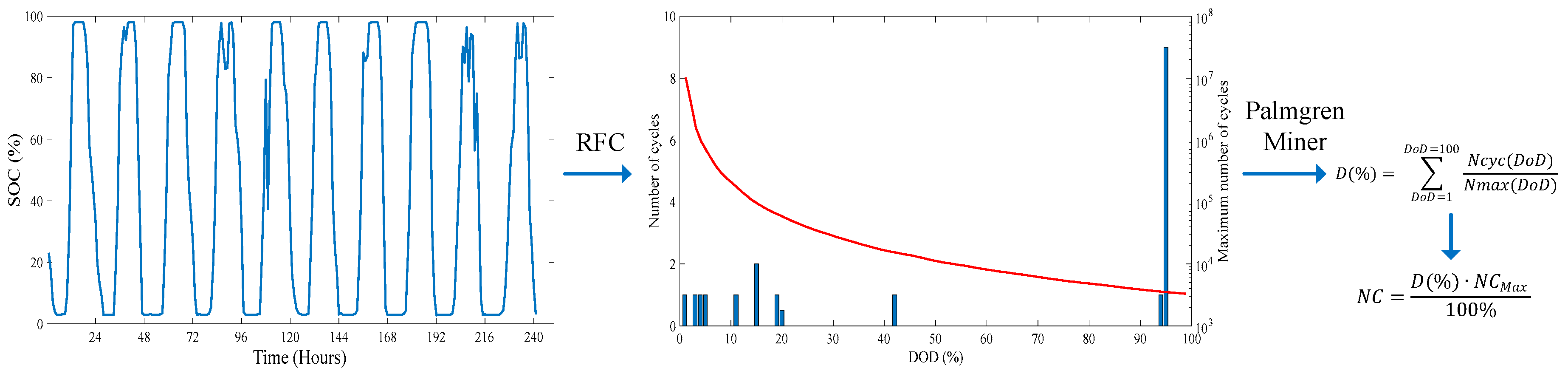
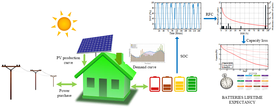
2.5. Operation of PV Systems with Batteries

As previously introduced, although home solar storage systems will be potentially used for a wide variety of grid services that will help in enhancing the profitability of their installation, these are mainly installed nowadays for energy arbitrage and peak shaving (also back-up in certain locations). However, and regardless of the operation goal of the system, the control algorithm in charge of solar storage system’s operation must, at every given moment, analyze the difference between two uncontrollable variables ($P_{PV}$ and the consumption of the loads, $P_{load}$) and decide what to do if there is an excess or a shortage in power as a function of the main operational goal. In the first case, it can either charge the battery ($P_{ES}<0$) or sell energy to the grid ($P_{grid}<0$). In the second, it can supplement the power that is produced by the PV panels with energy stored (if available) or by purchasing from the grid. In an electricity market with a time-of-use rates structure (on-peak and off-peak hours) the control algorithm must take this decision by considering not only the current moment in time, but also the expected evolution of $P_{PV}$ and $P_{load}$. Otherwise, the implemented strategy could avoid purchasing energy during off-peak hours, only to have to buy it in the future, during on-peak periods. Such a problem can be easily formulated in the framework of Model Predictive Control (MPC) [52]. This is a controller design technique that is based on an optimization strategy, in which the future outputs for a given horizon N, called the prediction horizon, are predicted at each instant while using appropriate models. These predicted outputs depend on future decision variables, which are calculated by optimizing a determined criterion while fulfilling a set of constraints. Although a complete sequence of future decision variables is computed, only the first one is effectively sent to the system, because, at the next sampling instant, new information will be available. This is known as receding horizon.

For the problem at hand, which focused on the energy arbitrage, the economic balance of the energy exchanged with the grid mainly determines the optimization criterion. Regarding the constraints, the power balance, including powers from the PV system, the battery, the grid, and the loads, must be met; also, the state of charge (SOC) of the battery must be kept within its limits; and, finally, the power exchanged both with the grid and with the battery must also stay within certain limits, either because of power converters limitations or peak shaving strategies. Note that, even though $P_{ES}$ does not appear in the optimization cost, it is still a decision variable and it affects the results because of the constraints.

Taking all of these considerations into account, and following an approach similar to that in [53], the optimization problem to be solved in the MPC framework can be formulated as:

$$\min J_N={\displaystyle \sum }_{k=0}^{N}T\times c_{grid}\left(t+k\right)\times P_{grid}\left(t+k\right)$$

(7)

subject for $k=0\dots N$ to:

$${\widehat{P}}_{PV}\left(t+k\right)+P_{grid}\left(t+k\right)+P_{ES}\left(t+k\right)={\widehat{P}}_{load}\left(t+k\right)$$

$$E_{ES}\left(t+k+1\right)=E_{ES}\left(t+k\right)-T\times P_{ES}\left(t+k\right)$$

$$E_{ES,min}\le E_{ES}\left(t+k\right)\le E_{ES,max}$$

$$P_{ES,min}\le P_{ES}\left(t+k\right)\le P_{ES,max}$$

$$P_{grid,min}\le P_{grid}\left(t+k\right)\le P_{grid,max}$$

where:

• T is the sampling period.
• ${\widehat{P}}_{PV}\left(t+k\right)$ and ${\widehat{P}}_{load}\left(t+k\right)$ are the predictions for $P_{PV}\left(t+k\right)$ and $P_{load}\left(t+k\right)$, respectively.
• $P_{grid}\left(t+k\right)$ is the power exchanged with the grid at instant $t+k$, with $P_{grid}\left(t+k\right)>0$ when energy is purchased.
• $P_{ES}\left(t+k\right)$ is the power exchanged by the battery at instant $t+k$, with $P_{ES}\left(t+k\right)>0$ when discharging.
• $E_{ES}\left(t+k\right)$ is the energy available in the battery at instant $t+k$.
• $P_{ES,min}$ and $P_{ES,max}$ are the lower and upper bounds for the power exchanged with the ESS. These constraints are due to the limitations on the power converters and, therefore: $P_{ES,min}=P_{ES,max}$.
• $P_{grid,min}$ and $P_{grid,max}$ are the lower and upper bounds for the power exchanged with the grid ($P_{grid,min}=P_{grid,max}$). These can also represent limitations on a converter or can be used in order to implement peak shaving.
• $E_{ES,min}$ and $E_{ES,max}$ are the limits in between which the battery SOC must be kept.
• $c_{grid}=\{\begin{array}{cc}{c}_{buy}\left(h\right)& for P_{grid}>0\\ c_{sell}& for P_{grid}<0\end{array}$ are the electricity prices. $c_{buy}$ changes its values with the hour of the day $h$ depending on the rate period (on-peak or off-peak), while $c_{sell}$ is considered constant and $c_{buy}\left(h\right)>c_{sell}$ for any given $h$.

In this work, the described optimization is performed hourly, updating the problem with the new measurements of $E_{ES}\left(t\right)$ at each step, and also ${\widehat{P}}_{PV}\left(t+k\right)$ when new information is available.

Although most of the equations in the above problems are linear, such a problem in its current formulation is still difficult to solve because of the piecewise nature of $c_{grid}.$ This kind of functions can be dealt with by introducing binary variables, which lead to a mixed integer linear program (MILP), which is computationally prohibitive for the problem size. Therefore, a different formulation is proposed. The idea is to replace $P_{grid}$ by two new variables, $P_{buy}$ and $P_{sell}$, for the cases when it is positive or negative, which yields the following problem:

$$\min J_N={\displaystyle \sum }_{k=0}^{N}T\left(c_{buy}\left(t+k\right)P_{buy}\left(t+k\right)-c_{sell}\left(t+k\right)P_{sell}\left(t+k\right)\right)$$

(8)

subject for $k=0\dots N$ to:

$${\widehat{P}}_{PV}\left(t+k\right)+P_{buy}\left(t+k\right)+P_{ES}\left(t+k\right)={\widehat{P}}_{load}\left(t+k\right)+P_{sell}\left(t+k\right)$$

$$E_{ES}\left(t+k+1\right)=E_{ES}\left(t+k\right)-T\times P_{ES}\left(t+k\right)$$

$$E_{ES,min}\le E_{ES}\left(t+k\right)\le E_{ES,max}$$

$$0\le P_{buy}\left(t+k\right)\le P_{grid,max}$$

$$0\le P_{sell}\left(t+k\right)\le -P_{grid,min}$$

$$P_{ES,min}\le P_{ES}\left(t+k\right)\le P_{ES,max}$$

$$P_{buy}\left(t+k\right)·P_{sell}\left(t+k\right)=0,$$

where the last quadratic constraint is the only one not linear, being introduced to avoid the suboptimal solution in which energy is simultaneously bought and sold from the grid.

Then, let us consider a new optimization problem by dropping this last constraint that involves $P_{buy}$ and $P_{sell}$. Because of the structure of this new problem, its optimal solution is such that either $P_{buy}^{opt}=0$ or $P_{sell}^{opt}=0$. Indeed, if $P_{buy}^{opt}\ne 0$ and $P_{sell}^{opt}\ne 0,$ as ${\mathrm{c}}_{\mathrm{buy}}>{\mathrm{c}}_{\mathrm{sell}}>0$, there would exist a new feasible solution $P^{\prime }{}_{buy}^{opt}=P_{buy}^{opt}-P_{sell}^{opt}$ and ${{\mathrm{P}}^{\prime }}_{\mathrm{sell}}^{\mathrm{opt}}=0$ with a lower value of the cost function, rendering $P_{buy}^{opt}$ and $P_{sell}^{opt}$ as being suboptimal. Furthermore, the new problem, with both the cost function and constraints defined as linear functions, is a linear program (LP), which is a convex optimization problem. Convexity implies that the optimization algorithm will find $P^{\prime }{}_{buy}^{opt}$ and $P^{\prime }{}_{sell}^{opt}$ instead of the suboptimal solutions. Therefore, this new linear program (LP) can replace the original optimization problem, which achieves the same optimal solutions and is easily solved with standard optimization tools.

Finally, it is important to remind that, for the application of the MPC strategy, prediction models ${\widehat{P}}_{PV}$ and ${\widehat{P}}_{load}$ are needed.

Regarding ${\widehat{P}}_{PV}$, it is predicted in this work from the PV system rated power and efficiency in combination with irradiance forecasted values downloaded from the models available online at the European Centre for Medium-Range Weather Forecasts (ECMWF) [54]. ECMWF produces an ensemble of predictions that indicate the likelihood of a range of future weather scenarios. Forecasts are made while using NWP methods, which have good performances for day-ahead forecasts and beyond. The forecasts predict the next 10 days with one-hour time steps, and updated forecasts are available every 12 hours, at 12 a.m. and 12 p.m. The spatial resolution of the forecasts is 0.1° for both latitude and longitude.

On the other hand, given the Southern European location of the households under analysis, ${\widehat{P}}_{load}$ is obtained as one of the reference load profiles defined by the Spanish Ministry of Industry for the residential sector [55]. Energy retailers in the Iberian Market use these profiles to bill those consumers not updated yet with consumption telemetry, and are therefore supposed to represent the average trends. Among the various profiles that are defined in [55], this work uses that designated for users with time-of-use electricity rates, which are those that are prone to be eligible by consumers with home solar storage systems. The blue continuous line in Figure 4 represents the annually averaged daily distribution of that load profile.

3. Results and Discussion

The analysis of the lifetime expectancy that is offered by the different types of Li-ion batteries has been performed by means of simulations while using MATLAB^®. According to the introduced control algorithm, the operation of the home storage system produces successive changes in the battery SOC that basically depend on the power balance to be granted hour after hour. Therefore, the continuous PV production and the household load values strongly characterize the SOC evolution.

In this sense, with the aim to try to generalize the results, the operation of the home storage systems at three different locations in Southern Europe during up to three years was explored (2016, 2017, 2018). Thus, up to nine annual irradiance patterns, presenting all of them around 1500 peak sun hours (PSH) per year on the horizontal plane, were available and evaluated. The three places used for analysis were: a location in the eastern part of Spain (on the Mediterranean coast at sea level, labelled as A), a location in the central plateau (800 m above sea level, labelled as B), and a location in the northern part of the country (420 m above sea level, labelled as C), respectively. With the same goal, three types of residential load patterns, those whose annually averaged hourly distributions are introduced in Figure 5, were analyzed. Note how one of them is practically coincident with the reference load distribution model that is provided in [55], that of household 3, while the other two load patterns represent users with significant consumption during the mornings, household 1, or during the evenings, household 2. Also note that, although being differently distributed throughout the day, the actual stochastic consumption of each of the households day after day adds up to an overall annual consumption of around 5000 kWh/year.

Moreover, an actual time-off-use tariff for residential consumers presenting daily off-peak (from 10 pm till noon) and on-peak (from noon till 10 pm) hours, regardless of the different seasons of the year was implemented. This comprehends the costs or prices that are summarized in

Table 2. Costs, in c€/kWh, of the electricity for the residential electricity tariff considered.

Period	On-Peak	Off-Peak
Purchase price (c€/kWh)	22	11
Sale price (c€/kWh)	5	5

for the purchase of electricity from the grid or for the injection of power into it. Note how the acquisition cost is always higher than the generation one.

Afterwards, simulations have been run for each of the combinations explained above. In all, if the three locations, the different years available, and the various load profiles are analyzed with each of the alternative home storage technological solutions, i.e., considering 2 kW or 4 kW rated PV installations at each household, and combining each of these PV systems with the various battery types analyzed (LFP, NMC…), which, in turn, are introduced with three different energy capacities (3.3 kWh, 6.5 kWh, and 10 kWh) and a roundtrip efficiency of 95%, these sum up 648 combinations. Note that the values of rated power for the PV plants simulated and the three different energy capacity ratings accounted for the batteries trying to reflect the most popular PV cases for residential installations in Europe and the usual battery storage commercial models being installed nowadays.

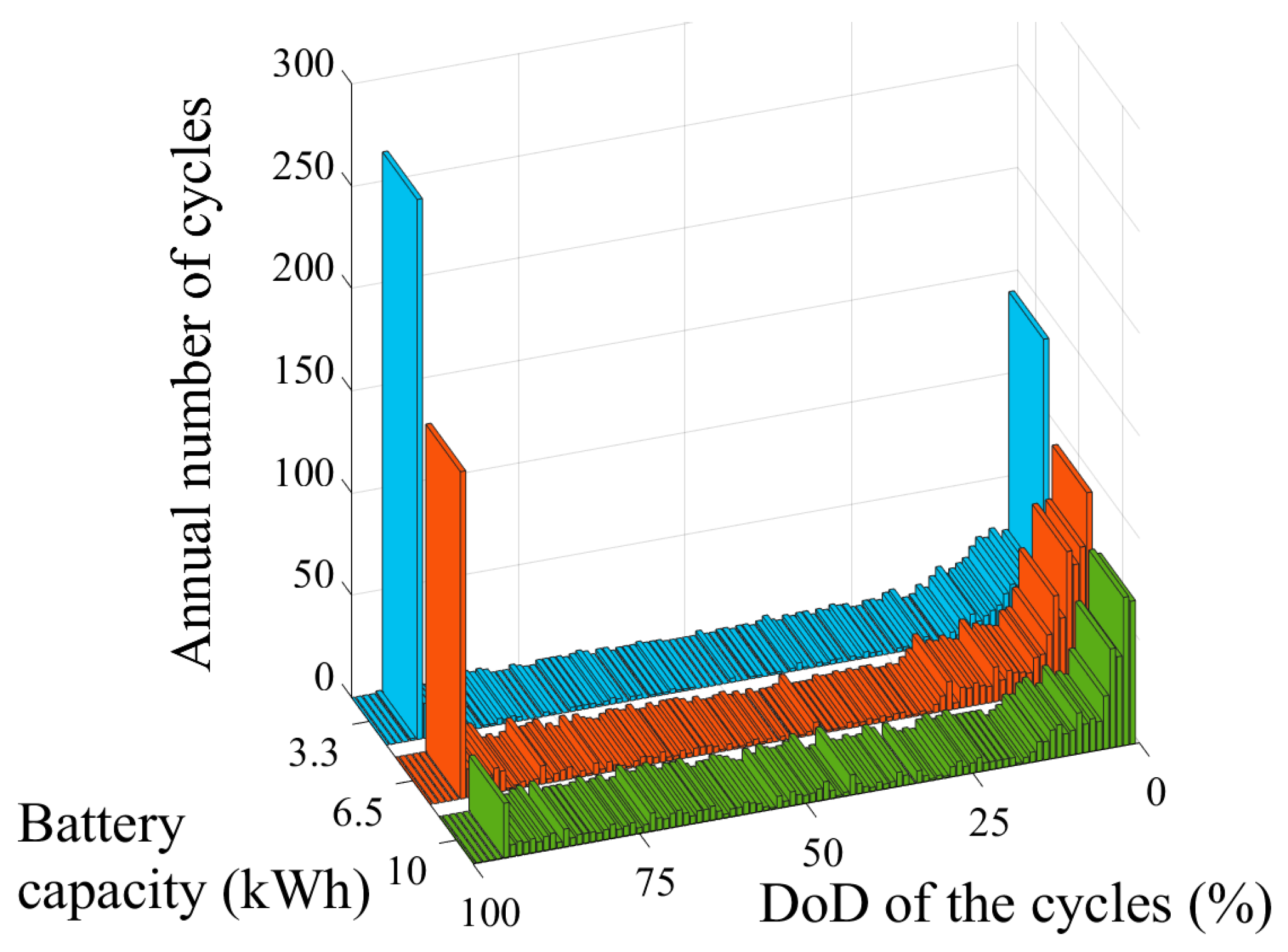
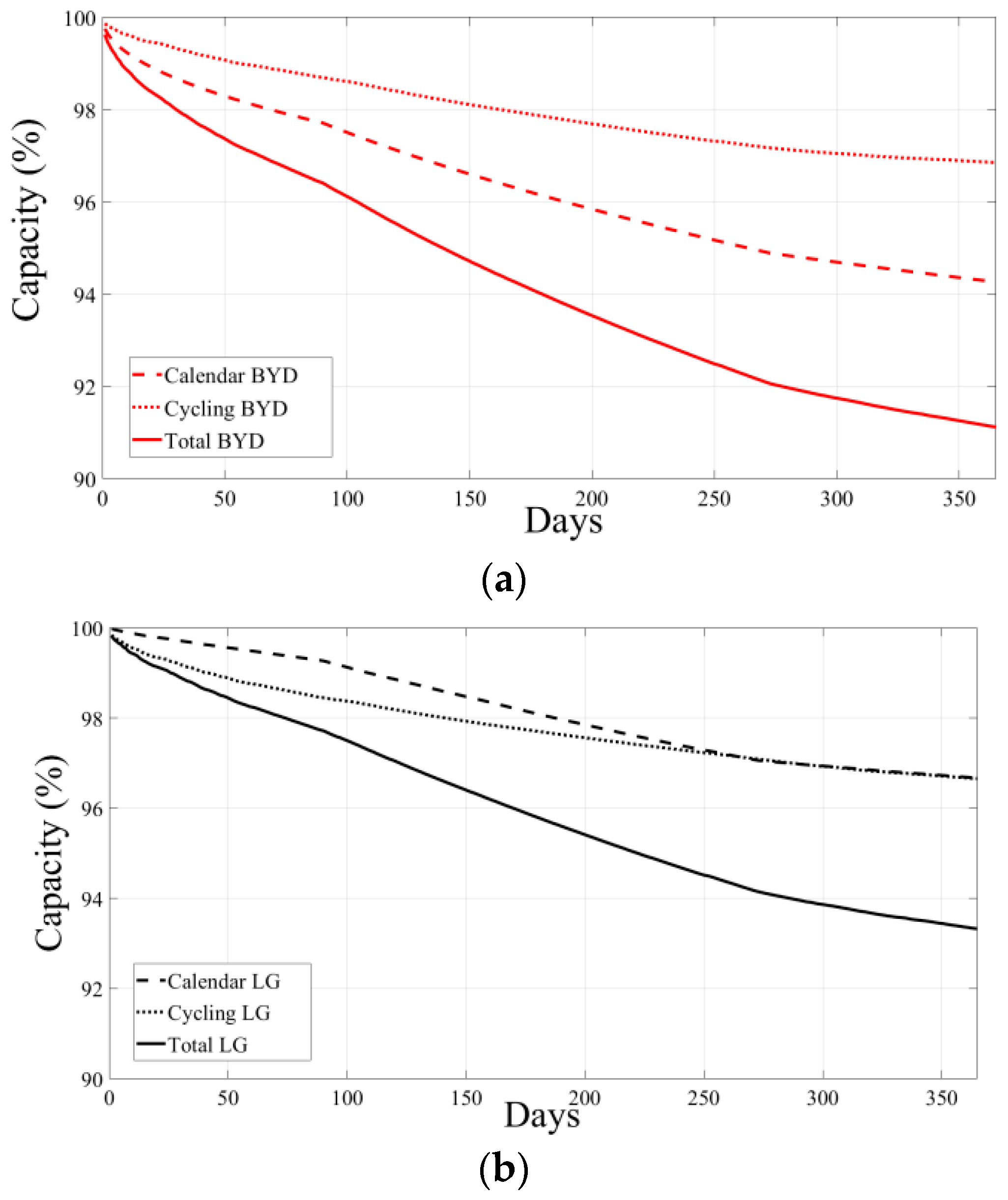
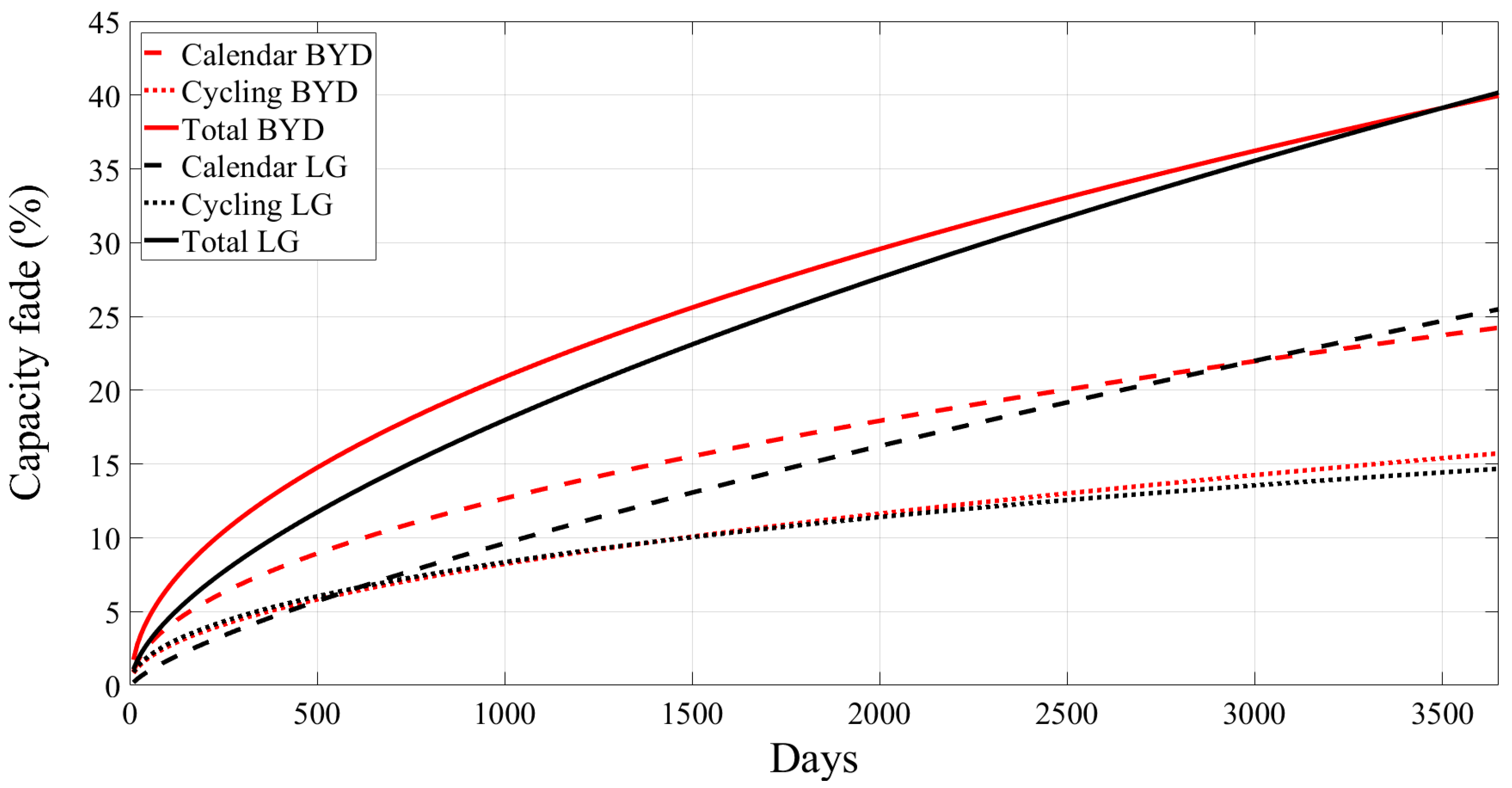
3.1. Annual Evolution of the Global Degradation

For each of the cases, an annual hourly simulation of the home solar storage system operation has been performed, providing the SOC evolution of the corresponding battery pack as main result. As explained in Section 2.1, the different SOC evolutions that were generated for the various battery capacities considered at a given household in one of the locations under study were, in turn, introduced into the RFC algorithm. This algorithm returned the histogram of partial charge-discharge cycles that were annually registered by the different batteries and the average SOC level for each cycle. Figure 6 represents such histograms generated, in that case, for household 1 in location A when a 4 kW rated-PV is assumed and for each of the three battery capacities considered (3.3 kWh, 6.5 kWh, and 10 kWh). It is important to notice in those depicted cycling patterns how the maximum depth of the charge-discharge cycles is 95%, limited in this way by the control system in agreement with manufacturer’s indication to avoid excessive degradation of the battery that is associated with very deep cycles. Apart from this main cycle, no significant partial cycles in terms of DoD are experienced by the home storage systems. Most of the partial cycles registered correspond to 25% and below DoD maneuvers. Adding them all, these do not even achieve in number the 95% DoD cycles. Therefore, home storage applications can be concluded to be very monotonous and sortable in terms of DoD patterns. Additionally, note how, as the battery capacity gets larger, the number of full cycles (those of 95% DoD) gets smaller and it is redistributed along all the range of partial DoDs. This directly impacts the cycle degradation of the different batteries. From these histograms, the amount of Q (charge throughput) that is experienced by the battery can be also estimated. In the same way, the ∅V and V values required for the calculations in equations (4) and (5) can be derived from the resulting average SOC provided by the RFC algorithm and from the SOC evolution itself, respectively. This is done by means of an experimental equation obtained for the battery packs measured in our lab that correlates the voltage of the battery pack with the corresponding SOC. Therefore, according to Equations (2) and (5), such a methodology is useful in the degradation analysis associated with the cycling.

Conversely, not being the only stress factor, temperature is considered to be the main one that is associated to calendar ageing though. For the cases that were simulated in this work, the batteries have been supposed to be stressed to cell operation temperatures always within the warranty limits and ranging from 35 °C to 45 °C along the year. These are defined for the cells as the temperature that would be achieved within the battery pack during regular operation when installed indoors at locations with air temperatures ranging from 20 °C to 32 °C. Therefore, the calendar ageing of the battery packs along the year can be equally estimated while using Equations (1) and (4).

Calendar and cycle ageing under these operation conditions are both represented for the first year of operation in Figure 7 for the commercial battery packs from BYD and LG Chem, respectively.

In agreement with the warranty evolution curves that are represented in Figure 4, note how the main difference among the battery degradation models is defined by their response in terms of calendar ageing. It can be clearly observed how, for the same operation conditions and, accordingly, the corresponding similar cycle ageing, the global degradation of the LFP battery is much more important than that of its NMC counterpart during the first year of operation due to the accelerated calendar ageing. However, this behavior becomes more balanced as time goes by, because of the relation with time of both calendar models (t^0.75 for NMC Vs. t^0.5 for LFP). This can be clearly deduced from Figure 3 and it is also reflected in the lifetime estimation values that are provided for the different chemistries in the different cases analyzed and summarized in the following subsection.

3.2. Comparative Discussion among Technologies.

Out of the 648 combinations analyzed, just some of them are introduced for discussion. The selected cases cover the main different operating scenarios and allow for extracting the main conclusions from this study. To start with,

Table 3. Lifetime expectancy results for the different batteries at household 1 in location A.

Model of Battery	PV Power (kW)	Battery Capacity (kWh)	Calendar Ageing EOL 70%	Cycling Ageing EOL 70%	Lifetime Expect. (years)	Calendar Ageing EOL 60%	Cycling Ageing EOL 60%	Lifetime Expect. (years)
LFP Ref	2	3.3	22.07	7.94	3.56	29.43	10.57	6.30
LFP Ref	2	6.5	22.82	7.19	3.76	30.41	9.59	6.63
LFP Ref	2	10	24.40	5.61	4.38	32.57	7.44	7.59
LFP Ref	4	3.3	22.09	7.92	3.57	29.47	10.53	6.32
LFP Ref	4	6.5	22.39	7.62	3.65	29.89	10.12	6.45
LFP Ref	4	10	23.40	6.60	4.01	31.22	8.78	7.02
LFP SoA	2	3.3	19.12	10.88	10.16	25.53	14.47	17,80
LFP SoA	2	6,5	20.00	10.01	11.06	26.69	13.32	19.48
LFP SoA	2	10	22.02	7.98	13.38	29.38	10.62	23.53
LFP SoA	4	3.3	19.15	10.85	10.20	25.56	14.45	17.85
LFP SoA	4	6.5	19.52	10.48	10.53	26.04	13.96	18.55
LFP SoA	4	10	20.73	9.27	11.81	27.67	12.33	20.88
NMC Ref	2	3.3	15.01	15.00	2.05	21.65	18.37	3.34
NMC Ref	2	6.5	17.55	12.45	2.87	24.86	15.15	4.57
NMC Ref	2	10	20.26	9.74	4.19	28.40	11.61	6.47
NMC Ref	4	3.3	15.60	14.40	2.07	22.37	17.64	3.33
NMC Ref	4	6.5	17.47	12.54	2.57	24.63	15.38	4.18
NMC Ref	4	10	19.76	10.25	3.08	27.73	12.28	4.65
NMC SoA	2	3.3	17.78	12.22	8.49	25.20	14.80	13.48
NMC SoA	2	6.5	19.98	10.02	11.58	27.93	12.07	18.18
NMC SoA	2	10	22.43	7.57	16.02	30.98	9.02	24.58
NMC SoA	4	3.3	18.27	11.73	8.41	25.80	14.20	13.31
NMC SoA	4	6.5	19.80	10.20	10.37	27.71	12.29	16.19
NMC SoA	4	10	21.85	8.15	11.57	30.23	9.77	17.75

introduces the lifetime expectancy results that were obtained in a given household (specific load curve) and a given location (irradiance profile) for the four battery models: those introduced in Section 2.1 and Section 2.2 as reference for LFP and NMC cells, respectively; and, those introduced in Section 2.3 as state-of-the-art (SoA) models. It is important to notice that the lifetime expectancy has been calculated assuming the EOL is achieved when the battery retains 70% (as defined for the reference cells in their catalogues) or 60% (as defined by manufacturers for the SoA battery packs). It can be observed at a glance how allowing the cells to operate until a 40% capacity fade offers a certainly increased lifetime expectancy. Therefore, although the warranties from manufacturers define different EOL horizons for the various cells, for the sake of comparison, both horizons have been analyzed for all of them.

It can be concluded from results in Table 3 that the SoA battery models significantly outperform their reference counterparts. The lifetimes for the SoA LFP battery are expected to be around three times those of the reference model, while a fourfold relation is registered between the NMC models. The improved properties of the new batteries in terms of expected lifetime actually enable them as a formal solution for residential storage, which was under discussion until recently due to the tight margin between their expected lifetimes and their payback periods (around 10 years, with highly dependence on the market). According to the results in Table 3, new battery developments would grant lifetime expectancies beyond 10 years for most of the cases simulated, even if only a 30% capacity fade is allowed to the battery prior to substitution.

When comparing the chemistries, it can be observed how the cycle ageing impacts more NMC cells than LFP ones; this makes the LFP batteries outfit NMC models when small battery packs are implemented in the home storage solution. This is because batteries will experience deep charge-discharge cycles every day due to their limited capacity. However, lifetime expectancies converge as battery capacity gets larger.

Beyond that, note how increasing the PV rated power from 2 kW to 4 kW do not significantly vary the expected lifetime when small size batteries are implemented (those of 3.3 kWh). It can introduce a 15% variation in the lifetime if the battery presents 10 kWh though. This is because 3.3 kWh batteries get regularly saturated (profit all their DoD) every day during the normal operation with any PV installation beyond 2 kW. Therefore, these cannot degrade faster due to cycling. On the contrary, 10 kWh batteries do not experience full discharge daily cycles with the 2 kW solar plant (reducing their cycle ageing), while they are more extensively profited, in terms of cycling, with the 4 kW plant. Finally, note that, as expected, the larger the battery size is the longer the lifetime expectancy results. This is due to the same reason just exposed and also explained with Figure 6, as the battery presents more capacity, cycles are shorter, and it suffers less from cycle ageing.

In order to analyze the impact of the local PV production (irradiance characteristics at the location), simulations both for different years at the same location (

Table 4. Lifetime expectancy results for the LFP state-of-the-art battery pack installed at household 3 analyzed with irradiance data from three successive years in location A.

Model of Battery	PV Power (kW)	Battery Capacity (kWh)	Lifetime Exp. Irradiance’16 (Years)	Lifetime Exp. Irradiance’17 (Years)	Lifetime Exp. Irradiance’18 (Years)
LFP SoA	2	3.3	18.96	18.99	18.64
LFP SoA	2	6.5	21.91	21.80	21.49
LFP SoA	2	10	25.90	25.82	25.52
LFP SoA	4	3.3	18.15	18.21	18.07
LFP SoA	4	6.5	19.26	19.14	19.01
LFP SoA	4	10	22.48	22.57	22.42

) and for the three different locations (

Table 5. Lifetime expectancy results for the NMC state-of-the-art battery pack installed at household 2 and analyzed at the three different locations.

Model of Battery	PV Power (kW)	Battery Capacity (kWh)	Lifetime Exp. Location A (years)	Lifetime Exp. Location B (Years)	Lifetime Exp. Location C (Years)
NMC SoA	2	3.3	13.50	13.12	12.93
NMC SoA	2	6.5	18.58	16.59	15.71
NMC SoA	2	10	25.43	21.45	19.81
NMC SoA	4	3.3	13.15	12.47	12.33
NMC SoA	4	6.5	16.09	14.98	14.35
NMC SoA	4	10	18.23	16.67	15.68

) have been carried out The first table introduces the lifetime expectancy that was obtained for the LFP battery pack installed, in that case, at household 3. This is analyzed with annual irradiance data from three successive years that were registered in the location labelled as A. Note in Table 4 how using a given year of annual irradiance data do not significantly impact the prognosis in terms of expected lifetime. The deviations are minimal. On the other hand, it can be observed in Table 5 how the different irradiance patterns registered at the various locations, although all of them with similar PSH, certainly influence the lifetime expectancy of the batteries. In this case, variability can range from 5% to 20%, depending on the location and, also, strongly on the size of the battery under analysis. However, in any of the cases, the battery packs keep presenting lifetimes beyond the 10-year warranty times.

Finally, the lifetime analysis of these Li-ion batteries is the influence of the load distribution or its variability is the other factor to take into consideration. The results in this sense are introduced in

Table 6. Lifetime expectancy results for the LFP and NMC state-of-the-art battery packs installed at location B in any of the households analyzed.

Model of Battery	PV Power (kW)	Battery Capacity (kWh)	Lifetime Exp. Household 1 (years)	Lifetime Exp. Household 2 (years)	Lifetime Exp. Household 3 (years)
LFP SoA	2	3.3	17.64	17.68	17.95
LFP SoA	2	6.5	18.67	18.79	20.13
LFP SoA	2	10	21.99	22.45	23.96
LFP SoA	4	3.3	17.62	17.61	17.66
LFP SoA	4	6.5	18.28	18.29	18.65
LFP SoA	4	10	20.72	21.16	22.27
NMC SoA	2	3.3	13.11	13.12	13.66
NMC SoA	2	6.5	16.44	16.59	18.60
NMC SoA	2	10	20.92	21.45	24.28
NMC SoA	4	3.3	12.55	12.47	12.77
NMC SoA	4	6.5	14.98	14.98	15.62
NMC SoA	4	10	16.55	16.67	17.38

. This table summarizes lifetime expectancies that were obtained for both the state-of-the-art LFP and NMC battery packs when installed, for this case, at location B and for each of the three households analyzed with their corresponding differently hourly-distributed loads, according to Figure 4. Note also again that the load profiles that are represented in Figure 4 are real and, therefore, also present different variabilities among the days throughout the year. Observe in Table 5 how the different load profiles (battery operation within the different households) imply lifetime deviations that are below 10% among the cases, and for each of the batteries. Therefore, the effect of the load can be concluded to be lower than that of the radiation on the lifetime expectancy analysis.

4. Conclusions

This paper introduces the lifetime expectancy for four different types of Li-ion batteries implemented as home solar storage systems. The chemistries analyzed are those that are being proposed nowadays for this kind of application by most of the manufacturers, i.e., LFP and NMC type batteries. For each of them, two types of cells have been considered: cells that were commercialized in the first half of this decade and state-of-the-art cells being used in commercial current solutions. The first presents degradation models in the literature that are used as reference for each of the chemistries, while the latter presents extended and improved operation warranties that are taken into account to update and calibrate new degradation models. Each of the four battery types has been analyzed in various scenarios of load pattern (three cases of distribution of the consumption along the day), at three different locations with their corresponding variations in the PV production profile. This is combined with two sizes of PV installation (2 kW and 4 kW) and with up to three levels of energy storage capacity (3.3 kWh, 6.5 kWh, and 10 kWh). Simulating the annual operation of the PV residential systems with batteries at each of the scenarios introduced and taking into account battery operation temperatures ranging from 35 °C to 45 °C, depending on the time of the year, is undertaken to perform the study. The introduction in the semi-empirical degradation models of the battery operation parameters (SOC evolutions, exchanged current, voltage stand-by levels, and others) obtained at the simulations, delivers lifetime expectancies for the different batteries under the various scenarios. In general, it can be observed how the cycle ageing impacts more NMC cells than LFP ones, which makes LFP batteries outfit NMC models when small battery packs are implemented in the home storage solution. However, as battery capacity gets larger, lifetime expectancies converge. Additionally, note that the degradation experienced for the different load profiles does not vary significantly, which implies that the warranty can be granted, regardless of the type of consumer. Additionally, similarly, the lifetime expectancy that is obtained at the different locations is also quite regular, which also implies that the warranty can be granted at any location. In fact, none of the cases analyzed provided lifetimes below 10 years being the battery pack temperature of simulations always below that of the warranty for state-of-the-art models. Neither charge throughput went beyond that offered in the manufacturers’ datasheets. Therefore, it can be finally concluded that current commercial battery models present lifetime expectancies under real operation conditions beyond the break-even point that is estimated, depending on the country and its corresponding electricity tariffs’ structures, between 8 and 12 years.

References

1. REN21. Renewables 2019 Global Status Report; REN21: Paris, France, 2019. [Google Scholar]
2. International Energy Agency (IEA). Tracking Progress on PV. 2019. Available online: https://www.iea.org/tcep/power/renewables/solarpv/ (accessed on 15 January 2020).
3. Joint Research Centre. European Comission. PV Status Report 2018; Publications Office of the European Union: Brussels, Belgium, 2018. [Google Scholar]
4. Bermudez, V. Electricity storage supporting PV competitiveness in a reliable and sustainable electric network. J. Renew. Sustain. Energy 2017, 9, 12301. [Google Scholar] [CrossRef] [Green Version]
5. Leadbetter, J.; Swan, L. Battery storage system for residential electricity peak demand shaving. Energy Build. 2012, 55, 685–692. [Google Scholar] [CrossRef]
6. Teng, F.; Strbac, G. Business cases for energy storage with multiple service provision. J. Mod. Power Syst. Clean Energy 2016, 4, 615–625. [Google Scholar] [CrossRef] [Green Version]
7. Hesse, H.C.; Schimpe, M.; Kucevic, D.; Jossen, A. Lithium-ion battery storage for the grid—A review of stationary battery storage system design tailored for applications in modern power grids. Energies 2017, 10, 2107. [Google Scholar] [CrossRef] [Green Version]
8. Wood Mackenzie. Global Energy Storage Outlook: Q3 2019; Wood Mackenzie: Edinburgh, UK, 2019. [Google Scholar]
9. International Renewable Energy Agency. Innovation Landscape Brief: Behind-the-Meter Batteries; International Renewable Energy Agency: Abu Dhabi, United Arab Emirates, 2019.
10. Wood Mackenzie. Europe Residential Energy Storage Outlook 2019–2024; Wood Mackenzie: Edinburgh, UK, 2019. [Google Scholar]
11. Weniger, J.; Tjaden, T.; Quaschning, V. Sizing of residential PV battery systems. Energy Procedia 2014, 46, 78–87. [Google Scholar] [CrossRef] [Green Version]
12. Tant, J.; Geth, F.; Six, D.; Tant, P.; Driesen, J. Multiobjective battery storage to improve PV integration in residential distribution grids. IEEE Trans. Sustain. Energy 2013, 4, 182–191. [Google Scholar] [CrossRef] [Green Version]
13. Hafiz, F.; de Queiroz, A.R.; Husain, I. Multi-stage stochastic optimization for a PV-storage hybrid unit in a household. In Proceedings of the 2017 IEEE Industry Applications Society Annual Meeting, Cincinnati, OH, USA, 1–5 October 2017. [Google Scholar]
14. Naumann, M.; Karl, R.C.; Truong, C.N.; Jossen, A.; Hesse, H.C. Lithium-ion battery cost analysis in PV-household application. Energy Procedia 2015, 73, 37–47. [Google Scholar] [CrossRef] [Green Version]
15. Sun, C.; Sun, F.; Moura, S.J. Nonlinear predictive energy management of residential buildings with photovoltaics & batteries. J. Power Sources 2016, 325, 723–731. [Google Scholar]
16. Segarra-Tamarit, J.; Perez, E.; Alfonso-Gil, J.C.; Arino, C.; Aparicio, N.; Beltran, H. Optimized management of a residential microgrid using a solar power estimation database. In Proceedings of the 2017 IEEE 26th International Symposium on Industrial Electronics, Edinburgh, UK, 19–21 June 2017. [Google Scholar]
17. Barcellona, S.; Piegari, L.; Musolino, V.; Ballif, C. Economic viability for residential battery storage systems in grid-connected PV plants. IET Renew. Power Gener. 2018, 12, 135–142. [Google Scholar] [CrossRef]
18. Munzke, N.; Schwarz, B.; Barry, J. The Impact of Control Strategies on the Performance and Profitability of Li-Ion Home Storage Systems. Energy Procedia 2017, 135, 472–481. [Google Scholar] [CrossRef]
19. Beltran, H.; Garcia, I.T.; Alfonso-Gil, J.C.; Perez, E. Levelized Cost of Storage for Li-Ion Batteries Used in PV Power Plants for Ramp-Rate Control. IEEE Trans. Energy Convers. 2019, 34, 554–561. [Google Scholar] [CrossRef]
20. Kakimoto, N.; Satoh, H.; Takayama, S.; Nakamura, K. Ramp-Rate Control of Photovoltaic Generator With Electric Double-Layer Capacitor. IEEE Trans. Energy Convers. 2009, 24, 465–473. [Google Scholar] [CrossRef]
21. Du, Y.; Jain, R.; Lukic, S.M. A novel approach towards energy storage system sizing considering battery degradation. In Proceedings of the 2016 IEEE Energy Conversion Congress and Exposition, Milwaukee, WI, USA, 18–22 September 2016; pp. 1–8. [Google Scholar]
22. Swierczynski, M.; Stroe, D.I.; Stan, A.I.; Teodorescu, R.; Sauer, D.U. Selection and performance-degradation modeling of LiMo2/Li4Ti5O12 and LiFePO4/C battery cells as suitable energy storage systems for grid integration with wind power plants: An example for the primary frequency regulation service. IEEE Trans. Sustain. Energy 2014, 5, 90–101. [Google Scholar] [CrossRef]
23. Wankmüller, F.; Thimmapuram, P.R.; Gallagher, K.G.; Botterud, A. Impact of battery degradation on energy arbitrage revenue of grid-level energy storage. J. Energy Storage 2017, 10, 56–66. [Google Scholar] [CrossRef] [Green Version]
24. Berglund, F.; Zaferanlouei, S.; Korpas, M.; Uhlen, K. Optimal operation of battery storage for a subscribed capacity-based power tariff prosumer—A Norwegian case study. Energies 2019, 12, 4450. [Google Scholar] [CrossRef] [Green Version]
25. Hoke, A.; Brissette, A.; Smith, K.; Pratt, A.; Maksimovic, D. Accounting for lithium-ion battery degradation in electric vehicle charging optimization. IEEE J. Emerg. Sel. Top. Power Electron. 2014, 2, 691–700. [Google Scholar] [CrossRef]
26. Grün, T.; Stella, K.; Wollersheim, O. Impacts on load distribution and ageing in Lithium-ion home storage systems. Energy Procedia 2017, 135, 236–248. [Google Scholar] [CrossRef]
27. Angenendt, G.; Zurmühlen, S.; Mir-Montazeri, R.; Magnor, D.; Sauer, D.U. Enhancing Battery Lifetime in PV Battery Home Storage System Using Forecast Based Operating Strategies. Energy Procedia 2016, 99, 80–88. [Google Scholar] [CrossRef] [Green Version]
28. Abdulla, K.; De Hoog, J.; Muenzel, V.; Suits, F.; Steer, K.; Wirth, A.; Halgamuge, S. Optimal Operation of Energy Storage Systems Considering Forecasts and Battery Degradation. IEEE Trans. Smart Grid 2018, 9, 2086–2096. [Google Scholar] [CrossRef]
29. Hesse, H.C.; Martins, R.; Musilek, P.; Naumann, M.; Truong, C.N.; Jossen, A. Economic optimization of component sizing for residential battery storage systems. Energies 2017, 10, 835. [Google Scholar] [CrossRef]
30. Vieira, F.M.; Moura, P.S.; de Almeida, A.T. Energy storage system for self-consumption of photovoltaic energy in residential zero energy buildings. Renew. Energy 2017, 103, 308–320. [Google Scholar] [CrossRef]
31. Castillo-Cagigal, M.; Caamano-Martín, E.; Matallanas, E.; Masa-Bote, D.; Gutiérrez, A.; Monasterio-Huelin, F.; Jiménez-Leube, J. PV self-consumption optimization with storage and Active DSM for the residential sector. Sol. Energy 2011, 85, 2338–2348. [Google Scholar] [CrossRef] [Green Version]
32. Telaretti, E.; Ippolito, M.; Dusonchet, L. A simple operating strategy of small-scale battery energy storages for energy arbitrage under dynamic pricing tariffs. Energies 2016, 9, 12. [Google Scholar] [CrossRef] [Green Version]
33. Zhang, C.; Wei, Y.L.; Cao, P.F.; Lin, M.C. Energy storage system: Current studies on batteries and power condition system. Renew. Sustain. Energy Rev. 2018, 82, 3091–3106. [Google Scholar] [CrossRef]
34. Barré, A.; Deguilhem, B.; Grolleau, S.; Gérard, M.; Suard, F.; Riu, D. A review on lithium-ion battery ageing mechanisms and estimations for automotive applications. J. Power Sources 2013, 241, 680–689. [Google Scholar] [CrossRef] [Green Version]
35. Berecibar, M.; Gandiaga, I.; Villarreal, I.; Omar, N.; van Mierlo, J.; van den Bossche, P. Critical review of state of health estimation methods of Li-ion batteries for real applications. Renew. Sustain. Energy Rev. 2016, 56, 572–587. [Google Scholar] [CrossRef]
36. Baghdadi, I.; Briat, O.; Delétage, J.Y.; Gyan, P.; Vinassa, J.M. Lithium battery aging model based on Dakin’s degradation approach. J. Power Sources 2016, 325, 273–285. [Google Scholar] [CrossRef]
37. Cordoba-Arenas, A.; Onori, S.; Guezennec, Y.; Rizzoni, G. Capacity and power fade cycle-life model for plug-in hybrid electric vehicle lithium-ion battery cells containing blended spinel and layered-oxide positive electrodes. J. Power Sources 2015, 278, 473–483. [Google Scholar] [CrossRef] [Green Version]
38. Tang, L.; Rizzoni, G.; Onori, S. Energy management strategy for HEVs including battery life optimization. IEEE Trans. Transp. Electrif. 2015, 1, 211–222. [Google Scholar] [CrossRef]
39. Ecker, M.; Nieto, N.; Käbitz, S.; Schmalstieg, J.; Blanke, H.; Warnecke, A.; Sauer, D.U. Calendar and cycle life study of Li(NiMnCo)O2 -based 18650 lithium- ion batteries. J. Power Sources 2013, 248, 839–851. [Google Scholar] [CrossRef]
40. Vetter, J.; Novák, P.; Wagner, M.R.; Veit, C.; Möller, K.C.; Besenhard, J.O.; Winter, M.; Wohlfahrt-Mehrens, M.; Vogler, C.; Hammouche, A. Ageing mechanisms in lithium-ion batteries. J. Power Sources 2005, 147, 269–281. [Google Scholar] [CrossRef]
41. Delaille, A.; Grolleau, S.; Duclaud, F. SIMCAL Project: Calendar Aging Results Obtained on a Panel of 6 Commercial Li-Ion Cells. In Proceedings of the 224ème Electrochemical Energy Summit de l’Electrochemical Society, San Fransisco, CA, USA, October 2013. [Google Scholar]
42. Nishi, Y. Lithium-Ion Batteries. In Lithium-Ion Batteries, Science and Technologies; Masaki, Y.A., Brodd, R.J., Kozawa, A., Eds.; Springer: New York, NY, USA, 2014; pp. 21–39. [Google Scholar]
43. Li, J.; Wang, D.; Pecht, M. An electrochemical model for high C-rate conditions in lithium-ion batteries. J. Power Sources 2019, 436, 226885. [Google Scholar] [CrossRef]
44. Wu, Y.; Keil, P.; Schuster, S.F.; Jossen, A. Impact of Temperature and Discharge Rate on the Aging of a LiCoO2/LiNi0.8 Co0.15Al0.05O2 Lithium-Ion Pouch Cell. J. Electrochem. Soc. 2017, 164, A1438–A1445. [Google Scholar] [CrossRef]
45. Stroe, D.; Swierczynski, M.; Stan, A.; Teodorescu, R. Accelerated Lifetime Testing Methodology for Lifetime Estimation of Lithium-ion Batteries used in Augmented Wind Power Plants. IEEE Trans. Ind. Appl. 2014, 50, 690–698. [Google Scholar] [CrossRef]
46. SAFT Batteries. L41M Cell Datasheet. Available online: http://www.houseofbatteries.com/documents/VL41M.pdf (accessed on 21 November 2019).
47. Beltran, H.; Barahona, J.; Vidal, R.; Alfonso, J.C.; Ariño, C.; Pérez, E. Ageing of different types of batteries when enabling a PV power plant to enter electricity markets. In Proceedings of the IECON 2016—42nd Annual Conference of the IEEE Industrial Electronics Society, Florence, Italy, 23–26 October 2016; pp. 1986–1991. [Google Scholar]
48. Schmalstieg, J.; Käbitz, S.; Ecker, M.; Sauer, D.U. A holistic aging model for Li(NiMnCo)O2 based 18650 lithium-ion batteries. J. Power Sources 2014, 257, 325–334. [Google Scholar] [CrossRef]
49. Sanyo. UR18650E Cell Datasheet. Available online: https://www.master-instruments.com.au/products/62415/UR18650E.html (accessed on 21 November 2019).
50. BYD. BYD B-Box Limited Warranty Letter. 2018. Available online: https://solar-distribution.baywa-re.com.au/fileadmin/Solar_Distribution_AU/04_Products/03_Media/BYD/BYD_Battery-Box_LV_Warranty_Letter_Australia_.pdf (accessed on 21 November 2019).
51. LG Chem, RESU Battery Storage Systems Limited Warranty. 2018. Available online: https://www.sharp.es/cps/rde/xbcr/documents/documents/Service_Information/Warranty/RESU3.3-6.5-10-Limited-Warranty-EU-Standard-EN-v1.1-191030.pdf (accessed on 21 November 2019).
52. Camacho, E.F.; Bordons, C. Model Predictive Control; Springer: Berlin, Germany, 2004. [Google Scholar]
53. Perez, E.; Beltran, H.; Aparicio, N.; Rodriguez, P. Predictive power control for PV plants with energy storage. IEEE Trans. Sustain. Energy 2013, 4, 482–490. [Google Scholar] [CrossRef] [Green Version]
54. Molteni, F.; Buizza, R.; Palmer, T.N.; Petroliagis, T. The ECMWF Ensemble Prediction System: Methodology and validation. Q. J. R. Meteorol. Soc. 1996, 122, 73–119. [Google Scholar] [CrossRef]
55. Dirección General de Política Energética y Minas—Ministerio para la Transición Ecológica. In Resolución de 21 de Diciembre de 2018, por la que se Aprueba el Perfil de Consumo y el Método de Cálculo a Efectos de Liquidación de Energía; Boletín Oficial del Estado Español (BOE): Madrid, Spain, 2018; pp. 536–713.
Figure 1. Commonwealth Games Athlete’s Village in Glasgow (Scotland), by Solar Trade Association (CC BY-SA 2.0).
Energies 13 00568 g001
Figure 2. List of main home storage systems available in the market and type Li-ion cells implemented.
Energies 13 00568 g002
Figure 3. Definition of the equivalent number of full cycles (NC) from a partially cycled state of charge (SOC) evolution.
Energies 13 00568 g003
Figure 4. Degradation evolution throughout 10 years under warranty conditions for the two commercial Li-ion battery packs analyzed in this work.
Energies 13 00568 g004
Figure 5. Load distribution profile for the three households analyzed, and reference load curve used as model.
Energies 13 00568 g005
Figure 6. Histogram for the number of cycles for each depth of discharge (DoD) for three different battery capacities.
Energies 13 00568 g006
Figure 7. Cycling, calendar, and total capacity reduction in one year for a 3.3 kWh LiFePO4 (LFP) (a) and LiNiMn-CoO2 (NMC) (b) battery operated at location A within household 1.
Energies 13 00568 g007