Article

Development of a High-Resolution Wind Forecast System Based on the WRF Model and a Hybrid Kalman-Bayesian Filter

by
Carlos Otero-Casal
1,2,*,
Platon Patlakas
3,
Miguel A. Prósper
4,
George Galanis
5 and
Gonzalo Miguez-Macho
1
1
Nonlinear Physics Group, Universidade de Santiago de Compostela, 15705 Santiago de Compostela, Spain
2
MeteoGalicia, Xunta de Galicia, 15707 Santiago de Compostela, Spain
3
School of Physics, Division of Environment and Meteorology, University of Athens, 15784 Athens, Greece
4
Siemens Gamesa, Meteorology Department, 28043 Madrid, Spain
5
Mathematical Modeling and Applications Laboratory, Hellenic Naval Academy, Hatzikiriakion, 18539 Piraeus, Greece
*
Author to whom correspondence should be addressed.
Energies 2019, 12(16), 3050; https://doi.org/10.3390/en12163050
Submission received: 2 June 2019 / Revised: 22 July 2019 / Accepted: 29 July 2019 / Published: 8 August 2019
(This article belongs to the Special Issue Renewable Energy Resource Assessment and Forecasting)

Abstract

:
Regional microscale meteorological models have become a critical tool for wind farm production forecasting due to their capacity for resolving local flow dynamics. The high demand for reliable forecasting tools in the energy industry is the motivation for the development of an integrated system that combines the Weather Research and Forecasting (WRF) atmospheric model with an optimization obtained by the conjunction of a Kalman filter and a Bayesian model. This study focuses on the development and validation of this combined system in a very dense wind farm cluster located in Galicia (Northwest of Spain). A period of one year is simulated at 333 m horizontal resolution, with a daily operational forecasting set-up. The Kalman-Bayesian filter was tested both directly on wind speed and on the U-V (zonal and meridional) components for nowcasting periods from 10 min to 6 h periods, all of them with important applications in the wind industry. The results are quite promising, as the main statistical error indices are significantly improved in a 6 h forecasting horizon and even more in shorter horizon cases. The Mean Annual Error (MAE) for 1 h nowcasting horizon is 1.03 m/s for wind speed and 12.16 ° for wind direction. Moreover, the successful utilization of the integrated system in test cases with different characteristics demonstrates the potential utility that this tool may have for a variety of applications in wind farm operations and energy markets.

1. Introduction

The global expansion of wind energy is a well-known reality, especially in recent years. In fact, in 2017 52.5 GW of new wind power installations were added across the globe, bringing the total worldwide capacity up to 539 GW [1]. This was a record year for Europe as well, reaching record numbers with 15.6 GW of new wind power capacity installed [2]. Part of this success has derived from offshore wind farms and their new 3.1 GW in 2017. The market forecast predicts a continuation of this tendency for the next few years [1,3], establishing wind energy as one of the main ingredients of the worldwide energy mix, which translates into an increasing number of operational wind farms, composed of more powerful wind turbines.
Considering the aforementioned scenarios, an improvement of wind energy exploitation seems necessary, employing new strategies in future wind farm projections and better daily management of current installations. The latter is where high-resolution meteorological modeling becomes increasingly prominent. Local short-term forecasts can supply valuable information in an operational wind farm, as wind speed and direction predictions can lead to a better running of the installation [4,5] or even provide alert for any extreme weather situation such as a downslope windstorm [6] or a severe frost [7].
The Weather Research and Forecasting (WRF) meso and microscale model has been used extensively during the last few years in the wind energy field for a variety of applications [8,9,10]. It includes a wind turbine parameterization [11] enabling the study of the wake effect from wind turbines [5,12]. However, Numerical Weather Prediction (NWP) simulations by themselves, present some limitations regarding subgrid scale phenomena forecasting. Onshore farms can be affected by local climatology and microscale events with significant wind direction and intensity changes in short periods of time. It is well known that such variations cannot be well reproduced by NWP simulations with resolution lower than that of the small-scale events commented above. To address this problem, WRF Large Eddy Simulations (LES) have been shown to be useful modeling techniques within this field. Their high resolution (<100 m) allows obtaining a good characterization of the turbulent intensity and an accurate representation of the wind fields [13,14,15]. Despite these capabilities, the computational demands of this modeling methodology and its numerical instability over complex terrain [14,16] make it unfeasible for operational forecasting at the present time.
The combination of NWP and statistical post-processes, like Model Output Statistics (MOS) or dynamically adjustable filters, can be an effective technique to minimize errors induced by sub-grid phenomena and local effects. In this direction, several strategies have been developed. Kariniotakis and Pinson [17], Kariniotakis et al. [18] proposed a neural network approach while Vanem [19], Giebel [20], Resconi [21] and others introduce methodologies based on heavy statistical models. Another method adopted for the reduction of systematic biases that numerical weather prediction models face, is Kalman filtering based algorithms (Resconi [21], Pelland et al. [22], Galanis et al. [23,24], Crochet [25], Galanis and Anadranistakis [26], Kalnay [27], Kalman and Bucy [28], Kalman [29]). Stathopoulos et al. [30] used the combination of an ETA-coordinate weather prediction model (running at a resolution of 0.05 ° ) and a Kalman Filtering postprocess for wind power prediction. This showed an improved performance and favorable results. Hua et al. [31] use 3 km × 3 km WRF model simulations and a Kalman Filter to obtain more skillful wind speed forecasts. Che et al. [32], Che and Xiao [33] developed a similar forecasting system employing 0.5 km resolution WRF simulations with a Kalman filter for a wind farm in Japan. Despite the overall good performance, in many cases, such filters only reduce the systematic mean bias [34], especially in wind speed, due to the nature and variability of the parameter. A proposed solution for this drawback is described analytically in Galanis et al. [35]. The suggested optimization technique is emerging from the conjunction of a non-linear Kalman filter and a Bayesian model (K-B model). This new hybrid model led to promising results eliminating systematic biases in the model outputs and reducing the variability of the remaining white noise.
In this study, we develop and validate a combined system of WRF high-resolution simulations and the aforementioned K-B filter. The main novelty proposed is the application of the hybrid filter to the two-dimensional field of horizontal wind speed components instead of the 1-dimensional filter in Galanis et al. [35]. In this way, an improved prediction of wind speed and direction is produced for a very dense wind farm cluster located in Galicia (NW Spain). A period of one year, broken into 365 daily integrations, is simulated with the WRF atmospheric model at high resolution (333 m), and results are post-processed with the K-B filter.
The obtained integrated system is validated for different short-term forecast periods employing in-situ data from meteorological stations on the top of the wind turbines provided by the farm’s operator. In addition, the new wind direction nowcasting tool is applied to the wind energy field as a backup for the current yaw orientation systems, which are based on Supervisory Control And Data Acquisition (SCADA) data obtained from each wind turbine [36]. These sensors are sometimes affected by short temporal errors due to technical problems or severe meteorological situations. Apart from the wind farm operational issue, this kind of tool can be used by electric grid operators to prevent ramp event effects. These extreme short-term situations produce significant increases or drops in the power production [37], delivering a major impact on the grid.
The article is structured as follows: In Section 2 the methodology is explained in detail, with particular attention to the WRF model configuration and the K-B filter description. Section 3 discusses the results obtained for wind speed and wind direction nowcasting as well as applications on wind energy forecasting. Finally, in Section 4 conclusions are presented.

2. Methodology and Data

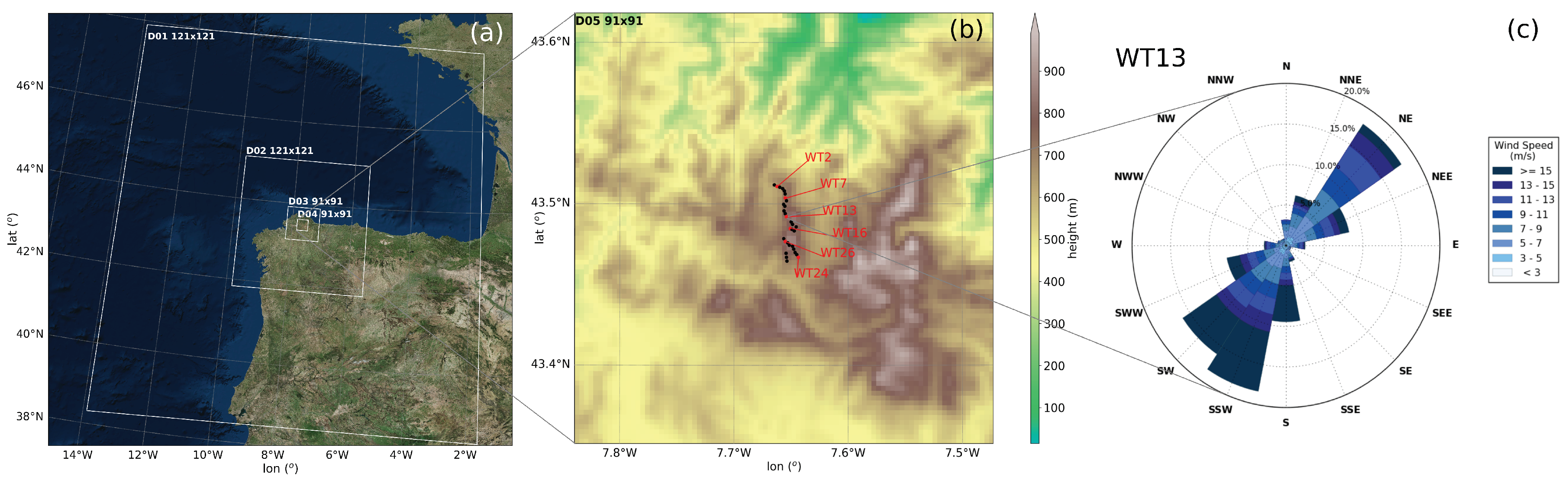
2.1. Wind Farm Location and WRF Configuration

Coruxeiras wind farm is located in Serra do Xistral mountains in Galicia, in northwest Spain (Figure 1a). The prevailing winds in this area are in the southwest/northeast direction (Figure 1c). In winter, frequent passing by cyclones along the North Atlantic storm track often produce strong southwest flows, whereas in summer, the poleward displacement of the subtropical Azores high, results in winds with a northeast component. Southeast/northeast flows are further accelerated due to the packing of the isobars by interaction with the high terrain of the northwestern Iberian Peninsula; hence the position of Serra do Xistral, exposed to the ocean in both prevailing directions, results in a very high wind energy potential. Numerous wind farms exist in the area, which is one of the most productive in Europe [38,39]. The developer and current operator of Coruxerias wind farm is Norvento S.L.U. company. It was installed in 2006 and is composed of 31 turbines with 60 m hub height and 74 m rotor diameter. They are separated by a mean distance of 300 m and placed along smooth hill tops of around 800 m elevation above sea level (Figure 1b).
For the atmospheric simulations, we use the Advanced Research WRF (ARW) model version 3.6 [40] (WRFV3.6), designed for operational forecasting, as well as research. WRFV3.6 is a limited-area mesoscale and microscale model based on a fully compressible and non-hydrostatic dynamic core [41] that uses a terrain-following hydrostatic-pressure vertical coordinate. Figure 1a shows the domain’s configuration where D01 is centered at 43.29 N and 7.75 W (Figure 1a) with 121 × 121 grid points of 9 km of horizontal resolution. The horizontal resolutions of D02, D03, and D04 are 3 km (121 × 121 grid points), 1 km (91 × 91 grid points) and 333 m (91 × 91 grid points) respectively. As demonstrated in Prósper et al. [5], the high horizontal resolution used over this complex terrain increases the accuracy of the wind forecast. The innermost domain has 67 vertical levels, 7 of which lie within the first 200 m above ground, at about 14, 41, 70, 99, 127, 156 and 184 m, a distribution that better captures wind and temperature variations in the surface layer [42] and improves the performance of the wind turbine parameterization [11]. Terrain elevation data is obtained from the ASTER Global Digital Elevation Map (GDEM) from USGS (United States Geological Survey) [43] with a resolution of 30 m, and land use information from the Corine (Coordination of Information on the Environment) database [44] with 250 m resolution.
A thorough validation of this model configuration for Coruxeiras wind farm and more information about the model physics options can be found in [5]. In the next table (Table 1), we present the main physics parameterizations used.
One year (2015/02/01–2016/02/01) of GFS forecast data from the National Centers for Environmental Prediction (NCEP) are used as initial and boundary conditions for the WRF model, with a 3-h update interval. The horizontal resolution of this dataset for all variables is 0.25 × 0.25 deg, with 32 levels ranging from 1000 to 10 hPa. The use of forecast data as boundary conditions should be particularly highlighted, as this study is performed employing a daily operational forecasting set-up, therefore including all the potential drawbacks of such an application.
Moreover, the A.C. Fitch wind turbine parameterization [11,52] is used in order to account for the wake effects of the turbines. Given the wind turbine dimensions, power curve, and their positions, the Fitch scheme represents them as momentum sinks, transferring the flow’s kinetic energy into turbulent kinetic energy and electricity.

2.2. Hybrid Bayesian Kalman Filter

In this subsection, the statistical optimization postprocess adopted is presented. Beginning with the polynomial Kalman filtering local adaptation model, the main goal is the estimation of the atmospheric model bias y t as a function of the model output m t .
y t = x 0 , t + x 1 , t · m t + v t
where x i , t ( i = 0 , 1 ) are the parameters to be estimated and v t is the Gaussian nonsystematic error.
The above equation can be expressed as y t = H t · x t + v t where x t = x 0 , t x 1 , t is the state vector and H t = 1 m t the observation matrix. As a result, it can be written in a more analytical way as follows:
y t = 1 m t · x 0 , t x 1 , t + v t
Similarly, the evolution in time of x t is described by the equation
x t = x t 1 + w t
where x t 1 is the parameter in t 1 and w t is the Gaussian nonsystematic error.
In the present study, a linear approach is followed, since it was found to be sufficient both in terms of reliability and computer resource needs. The estimation of the variables v t and w t is based on a training period. For this case and after multiple sensitivity tests, the training period was set to 140 include the last 12 values of the sample for each forecast. We note, however, that options such as the order of the polynomial in Equation (1) used or the training period, are case sensitive and depend on local features and time period characteristics.
In particular, the covariance matrices V t and W t of the error terms v t and w t are calculated as follows:
V t i = 1 11 i = 0 11 ( ( ( y t i H t i x t i ) ( i = 0 11 ( y t i H t i x t i ) 12 ) ) ) 2
W t i = 1 11 i = 0 11 ( ( ( x t i + 1 x t i ) ( i = 0 11 ( x t i + 1 x t i ) 12 ) ) ) 2
The main steps of the Kalman algorithm for the estimation of the state vector x t are summarized as follows:
  • A first estimation of x t is given by x t / t 1 = x t 1
  • The corresponding covariance matrix P t is calculated by P t / t 1 = P t 1 + W t
  • With a new observation y t available the calculation of x at time t takes the form: x t = x t / t 1 + K t ( y t H t x t / t 1 )
Here, K t = P t / t 1 H t T ( H t P t / t 1 H t T + V t ) 1 is the Kalman gain, a parameter that controls the flexibility of the filter.
More details on the Kalman filtering theory can be found in [27,28,29]. The filter has been tested successfully in wind speed and wind gust prediction Stathopoulos et al. [30], Louka et al. [34], Patlakas et al. [53], Galanis et al. [35] with results that ensure the reduction of the systematic errors induced by numerical weather models.
However, in most of the previous studies, the variation of the remaining nonsystematic part of the error is not reduced. For a further improvement of the Kalman filter output, we incorporate the following linear Bayesian model:
k t = o t + n t
where, k t represents the Kalman filtered output at time t (estimated by the Kalman filter as the model initial forecast corrected by y t ), o t is the corresponding observation value, and n t the remaining Gaussian nonsystematic white noise.
For the application of the Bayesian model, an approach based on Normal distribution is utilized based on the assumption that the probability density functions of the filter parameters have as follows: P ( o t ) N ( o μ , σ o 2 ) , P ( v t ) N ( 0 , σ v 2 ) . Then, the conditional pdf takes the form P ( k t | o t ) N ( o t , σ v 2 ) . The final estimation of the parameter o t takes advantage of the posteriori estimator given by o ^ t = a r g m a x P ( o t | k t ) .
Further details concerning Bayesian theory and models can be found in the studies of Box [54] and Bernardo and Smith [55], while the combination of the two approaches is fully described by Galanis et al. [35].
The new approach proposed in this work consists in the application of the K-B model for both wind speed and U-V components for different forecasting horizons, covering in this way both wind speed and direction with quite satisfactory results as presented in the following sections.

2.3. Observational Data and Nowcasting Experiments

The observational data used in this work is provided by Norvento S.L.U., collected from anemometers located on top of each turbine’s nacelle. Specifically, we use wind speed and wind direction (WS and WD hereafter) observations from six wind turbines, two in the north of the farm (WT2 and WT7), two in the center (WT13 and WT16) and two in the south (WT24 and WT26) (Figure 1b). In this way, the WRF K-B nowcasting tool is tested all over the wind farm, with each turbine differently affected by wake effects and local topography. One year of 10-min wind data for each turbine is available. We note that a priori quality control on the raw observational data is performed, filtering out discontinuities such as automatic starts after stops or preventive maintenance.
This leads to three different applications of the integrated forecasting model. More precisely, in the first scenario, the forecasting bias in WRF wind speed prediction is minimized by the Kalman filter described in the previous section based on the polynomial Equation (1). In a second step, the Bayesian component of the optimization procedure reduces the variability of the error, and therefore the forecasting uncertainty. Following the same concept, two different K-B filters are utilized separately for the U, V wind speed components. This scenario aims at the improvement of both the wind speed and direction simultaneously.
The period chosen for the present study is one year (1 February 2015–1 February 2016), divided into 365 daily simulations. Each run starts at 18 UTC the day before the one considered, and the initial 6 h are excluded from the forecast data series used in the analysis of the results, thus, only outputs after this spin-up time are taken into account.
By definition, nowcasting refers to short lead time weather forecasts. Some organizations like the U.S. National Weather Service stipulate that it pertains to lead times from zero to three hours. However, forecasts up to six hours are also considered nowcasts by different agencies [56]. To analyze the capabilities of our methodology, we evaluate the K-B filter with different nowcasting horizon periods, from 6 h to 10 min (Table 2) for each one of the daily simulations. For example, the wind speed nowcasting obtained in K-B 1 h is the result of correcting RAW data every 10 min by using model output and real data from one hour before. Results are compared with both observations and original non-post-processed WRF outputs.

3. Results and Discussion

The next section is divided into three parts; the first one analyzes the results obtained with the nowcasting wind speed postprocess at different time horizons, from 6 h to 10 min in advance. The analysis is developed for different temporal periods, from annual mean results to the performance of the experiments at individual simulation timesteps. The second subsection shows the results of the K-B filter used to measure wind direction correction, same as with wind speed, with different nowcasting horizons and mean errors for several periods. Finally, Section 3.3 shows an example of the improvement that K-B 1 h applied in wind direction could induce in the daily management of the studied wind farm.

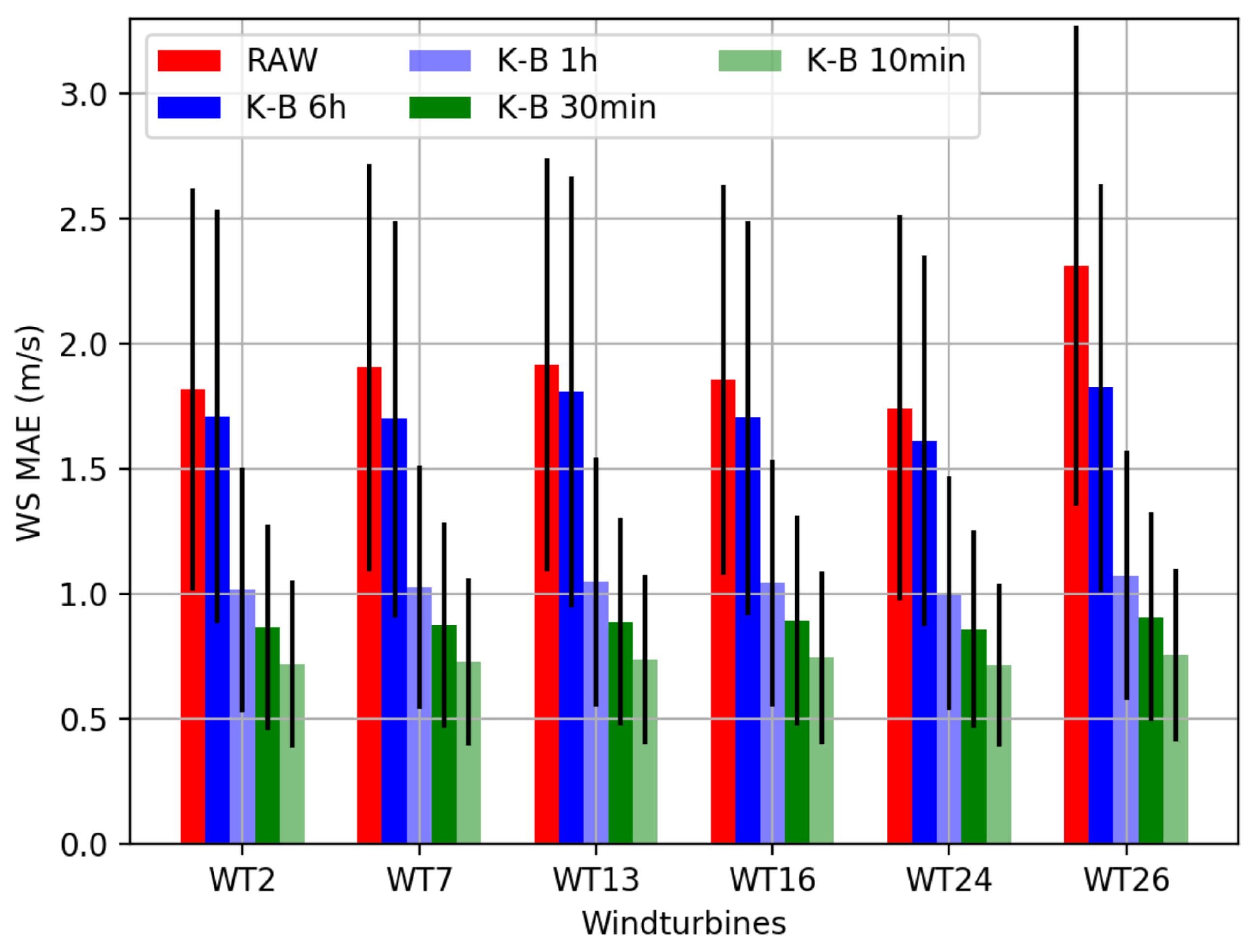
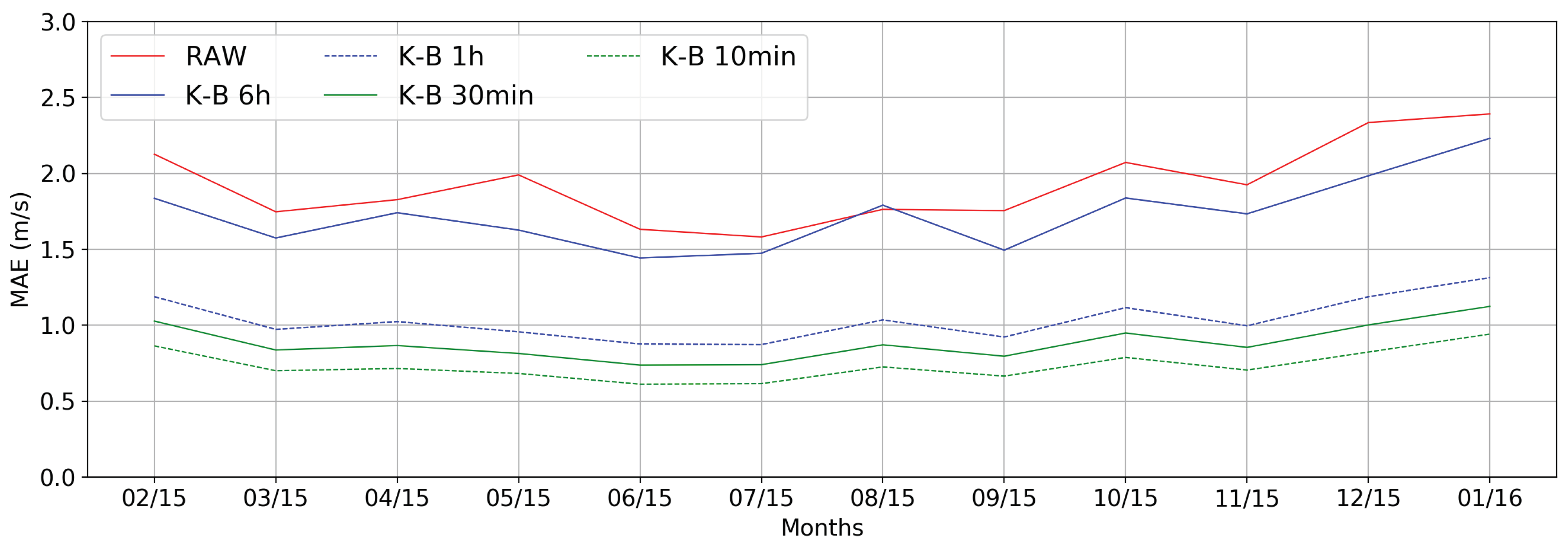
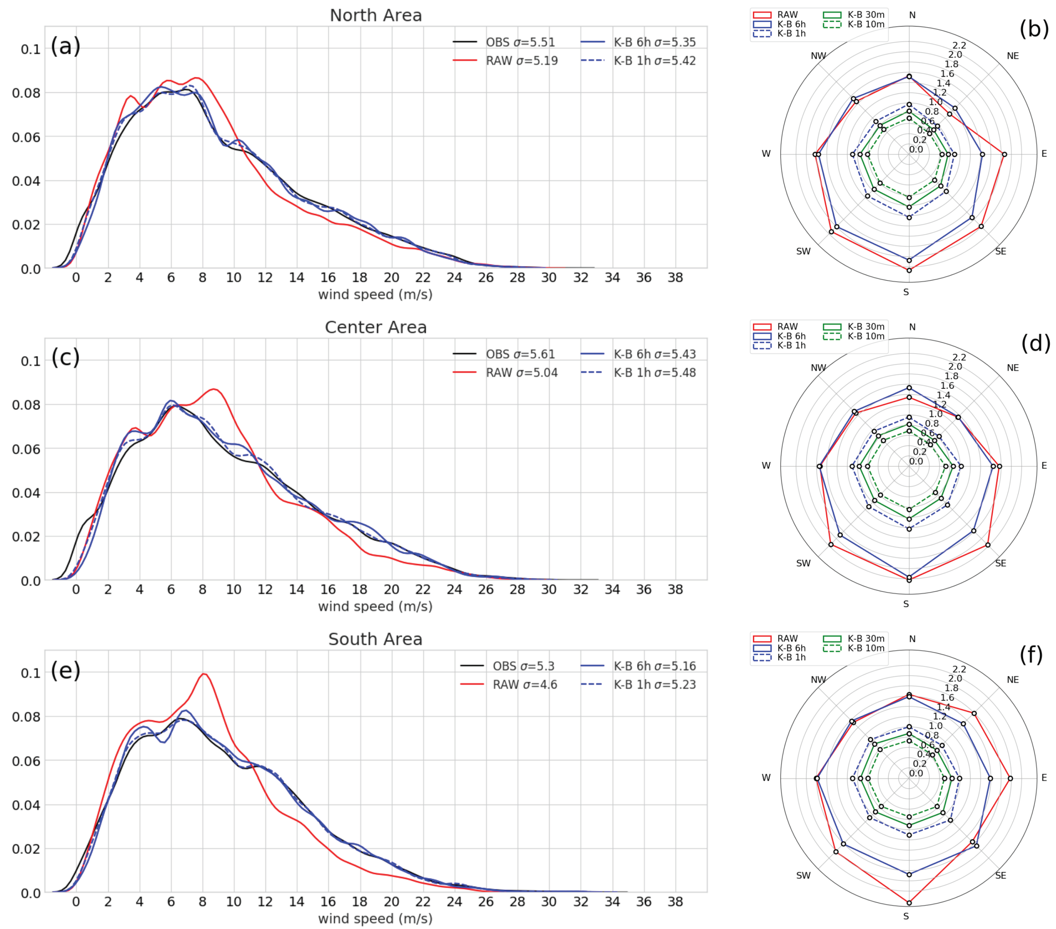
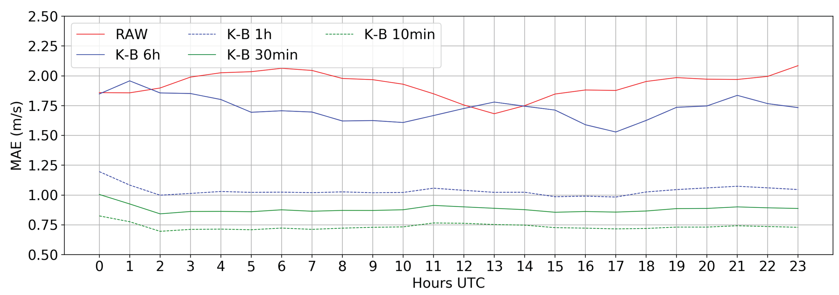
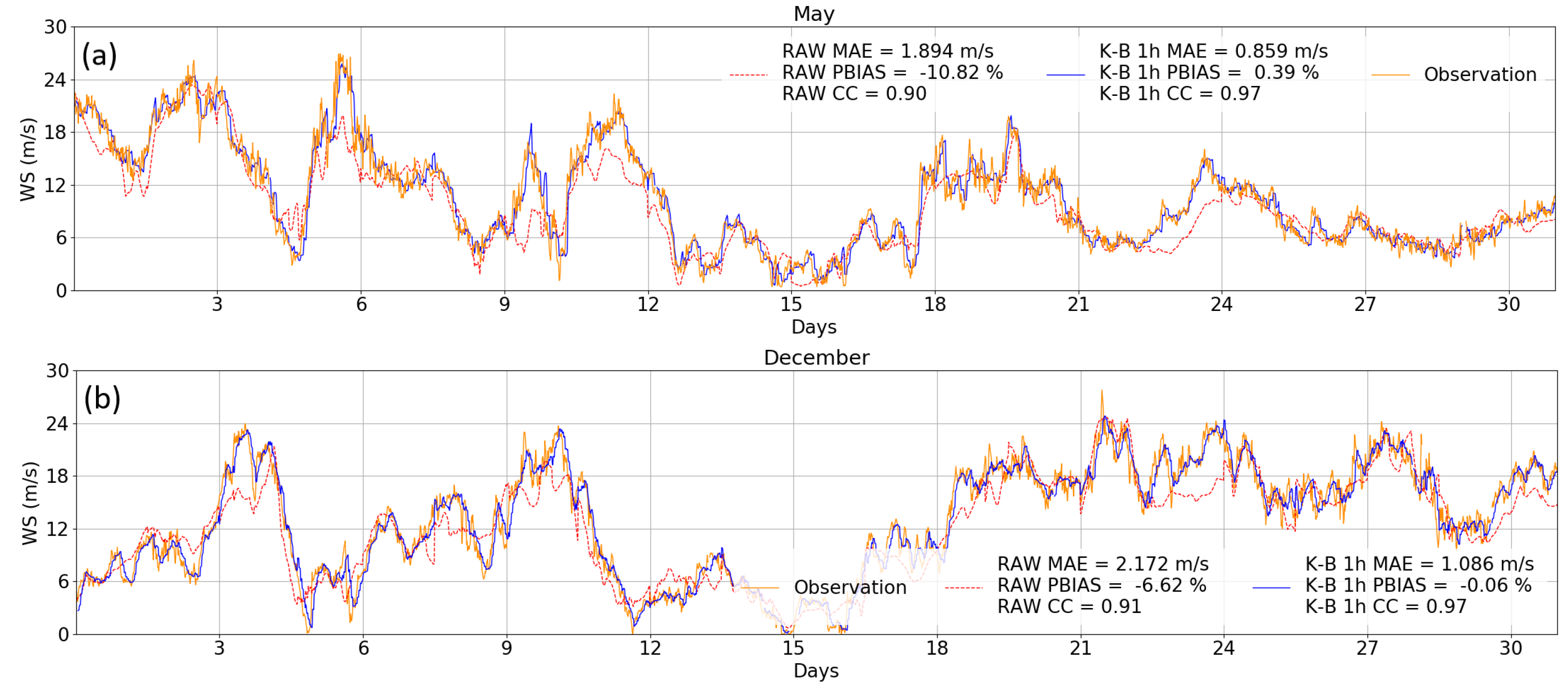
3.1. Wind Speed Nowcasting

This subsection employs several error measures at different temporal scales to provide a general view of the skill of all the experiments. The next equations show the statistical measures used in different temporal scales throughout the chapter.
M A E = 1 n i = 1 n f i o b i
M E = 1 n i = 1 n f i o b i
R M S E = i = 1 n f i o b i 2 n
σ = i = 1 n x i x ¯ 2 n
Equation (7) gives the Mean Absolute Error (MAE) between forecasts ( f i ) and observations ( o b i ), (8) the Mean Error (ME) estimating possible systematic biases, (9) the Root Mean Square Error (RMSE), where n is the sample size, and (10) the standard deviation ( σ ), where x i is the value, x the mean value of a study period.
Annual mean results are firstly shown in Figure 2, and Table 3 for each wind turbine studied. Figure 2 displays a bar chart with the annual WS MAE and standard deviation for each turbine and experiment performed. Table 3a,b present the annual WS ME and RMSE, again, for each turbine and experiment.
Overall, a similar improvement concerning WS MAE for all the wind turbines and cases is recorded. Raw WRF forecast MAEs are between 1.91 and 1.74 m/s, except for WT26, which has a RAW MAE of 2.31 m/s. All of these results, regardless of wind farm area, present a small reduction of the WS MAE (of around 10%) in the longest nowcast period, K-B 6 h (blue). It is important to highlight that the specific K-B approach employed in this experience is the result of training the tool for the nowcast time horizons analyzed. For this reason, apply this K-B tool configuration for a longer range, as for example K-B 24 h, would generate even worse than RAW case (K-B 24 h WS MAE = 2.37 m/s). Longer forecasting time ranges, as 24 h, are associated with different temporal-spatial scale wind phenomena and the sources of the errors for this temporal resolution are also different. If we want to use this K-B tool for 24 h or a longer horizon, it is necessary to perform a different training of the K-B for the points of interest. Continuing with Figure 2’s discussion, the accuracy of the K-B filter is significantly enhanced for shorter lead times, with K-B 1 h (pale blue) reaching a WS MAE of around 1 m/s in all cases. The shorter nowcasting periods, K-B 30 m (green) and K-B 10 m (pale green) show a further reduction of error, with values around 0.86 and 0.72 m/s respectively. The standard deviations plotted on top of each bar ( σ ) are also reduced for all turbines, in parallel with the shortening of the nowcasting periods. RAW cases have a mean σ of 0.82 m/s, and K-B 10 min present a mean value for all of the machines of 0.33 m/s.
The behavior of the WS ME is different as compared with MAE. All of the RAW WS MEs for the six wind turbines are negative, ranging from −0.33 m/s in WT13 to −1.40 in WT26. Unlike in WS MAEs, there is a clear difference between RAW and K-B 6 h MEs. In K-B 6 h cases, the ME practically disappears, with a value of 0.046 m/s. In the rest of the experiments, the ME is reduced even more; reaching a total ME of 0.005 m/s for the K-B 10 min case. WS RMSEs show a similar tendency to that of WS MAEs, with close mean values of the RAW and K-B 6 h experiments (2.54 and 2.36 m/s respectively) and a definite improvement between the three shorter nowcasting periods (K-B 1 h-30 min-10 min) and K-B 6 h.
Figure 3 analyzes the relationship between the observed and simulated wind field in terms of module and direction. As also discussed previously, there are similar error values and patterns in all of the wind turbines, which allows us to group them by areas while maintaining the rigor of the validation. In Figure 3a,c,e the wind speed distribution is displayed for the observations and the RAW, K-B 1 h and K-B 6 h experiments, for the North, Center and South areas respectively. Radar charts in Figure 3b,d,e depict the WS MAE as a function of direction for all experiments and areas.
The distribution plots in Figure 3a,c,e show a significant improvement from the K-B filter in the three areas. K-B 6 h mitigates the main wind speed deviations in all the range of the distributions. In the north area (Figure 3a) K-B filter cases correct a general overestimation from 6 to 10 m/s and an underestimation from 11 to 22 m/s. This behavior is repeated in the Central and South areas. K-B experiments (even K-B 6 h) obtain an important amelioration of the entire distribution shape, which is in agreement with the low ME errors shown in Table 3a. This demonstrates the reliability of the K-B filter in different wind situations, correcting under- and over-estimations indistinctively, which is vital for wind energy applications. Charts in Figure 3b,d,f show the skill of the K-B tool depending on wind direction. In RAW cases, the three areas present variations, as the general orientation of each zone and their position relative to the rest of the farm change forecast performance. K-B 6 h decreases mainly the higher directional errors as, for example, with southerly winds in the South area (Figure 3f). However, the K-B tool for 1 h, 30 min, and 10 min tends to smooth out errors from all sources, improving results in all the prevailing wind directions. Apart from the low MAE values observed, the symmetry in the figures in the shorter K-B time ranges leads to the conclusion that the tool is robust, rectifying wind errors in any regime. It presents the same good accuracy correcting northeast flows, principally produced in summer, as it does with southwesterly situations, characteristic of winter months.
The seasonal cycle of errors averaged for all the turbines is shown in Figure 4, comparing wind speed monthly MAE from RAW results with the same calculation from K-B experiments. Observed monthly mean wind speeds are also shown for reference in the table below (Table 4).
RAW MAEs are relatively constant throughout the year, with values around 2 m/s in all months. Slightly larger errors are observed in the winter period, when mean wind speeds are higher, and lower biases occur in summer months, when mean wind speeds are also lower. K-B 6 h obtains the biggest improvements in the months when the RAW error is largest, such as December or February and minor improvements in the summertime. This tendency to better improve bigger RAW MAE is also reflected in previous comparisons such as for WT26 in Figure 2 or the south radar chart in Figure 3f. In K-B experiments for shorter lead times, the pattern shown in Figure 3 is repeated, with a significant error decrease relative to K-B 6 h results and very similar outcomes in all K-B cases and months. The K-B 1 h MAEs are all very close to 1 m/s, February registers the higher K-B 1 h MAE, with 1.19 m/s and June the lowest, with 0.87 m/s. This equality among monthly errors is maintained in K-B 30 m and 10 m with mean values all year long around 0.88 and 0.73 m/s respectively.
After investigating the intra-annual behavior and monthly error patterns of the experiments, we examine their accuracy on a finer timescale. Figure 5 displays the mean hourly wind speed MAE during the simulated year for all the wind turbines analyzed in each experiment.
RAW error results present a daily cycle, with values of the MAE around noon lower than during the night. These differences among the hourly WS MAEs are, however, not very significant, and the lower absolute errors at noon seem to be related with the better representation of turbulent fluxes during that part of the day [5]. In contrast, K-B 6 h errors do not follow a daily cycle, attaining values below 1.75 m/s mostly during daytime, but obtaining a worse result than RAW at 01 and 13 UTC. K-B 1 h, 30 min, and 10 min present a very flat error pattern all day long. There are practically no differences among hourly results in these experiments. The situation is very similar to that in the monthly error plot (Figure 4); shorter term K-B cases represent a significant improvement with respect to K-B 6 h and RAW, and there is homogeneity in the entire error series in K-B 1 h, 30 min, and 10 min. The skill limit for the shorter term cases corresponds to a non-systematic part of the error, which is unavoidable for the filter.
The general conclusion reached from the different time scale and wind regime comparisons presented above is that the K-B filter at short-term erases any source of error. It achieves lower errors in all conditions, regardless of the intensity and direction of the wind or the time of day or season of the year. This uniformity in the corrections toward the elimination of the ME (Table 1) from short-term K-B cases, highlights the utility of this optimization module for wind energy purposes.
To illustrate the day-to-day results of the K-B nowcasting tool regarding wind speed at hub height, we show next comparisons between RAW, K-B 1 h, and observations for the Center area (WT13 and WT16 mean values) during the entire months of May and December. These months have the lowest and highest K-B 1 h MAE in this area respectively.
Disregarding some occasional large errors, the original WRF output (RAW) generally yields a good performance during the months shown, achieving MAEs below 2 m/s in both cases and PBIAS [57] of −10.82% in May and −6.62% in December (−6.59% for the whole year). Even considering these low RAW errors, which are extensive to all the yearly series, the K-B 1 h results represent an important improvement nonetheless. This is clearly apparent in these December and May plots (Figure 6), when the procedure successfully corrects forecast error by a factor of around 50%. KB-1 h PBIAS indicators, 0.39% in May and 0.06% in December, show a virtual disappearance of the original RAW subestimation, (0.21% for the whole year). Focusing on the correlation coefficient (CC), we can see that RAW case obtains a CC = 0.90 with respect to the observation. This value shows a high relationship between the observation and the RAW case. However, K-B 1 h improves the original RAW result reaching a CC = 0.97, which indicates an extremely high correlation between K-B 1 h nowcasting and observation data series. This indicator, combined with the MAE value for this same period (0.86 m/s), reflects an accurate performance of the K-B 1 h case. Total mean values for the wind farm along the whole year displays similar behavior as the example shown in the figure above. The mean CC for all wind turbines in WS RAW case is 0.91, and WS K-B 1 h obtains a CC = 0.97.
The nowcasting tool is able to produce better results at different time ranges regardless of the origin of the error, eliminating the most substantial deviations in any situation. Overall, the K-B filter exhibits a useful short-term operational forecasting performance, offering a stable improvement of the original WRF outputs during the whole year and for all the wind turbines.

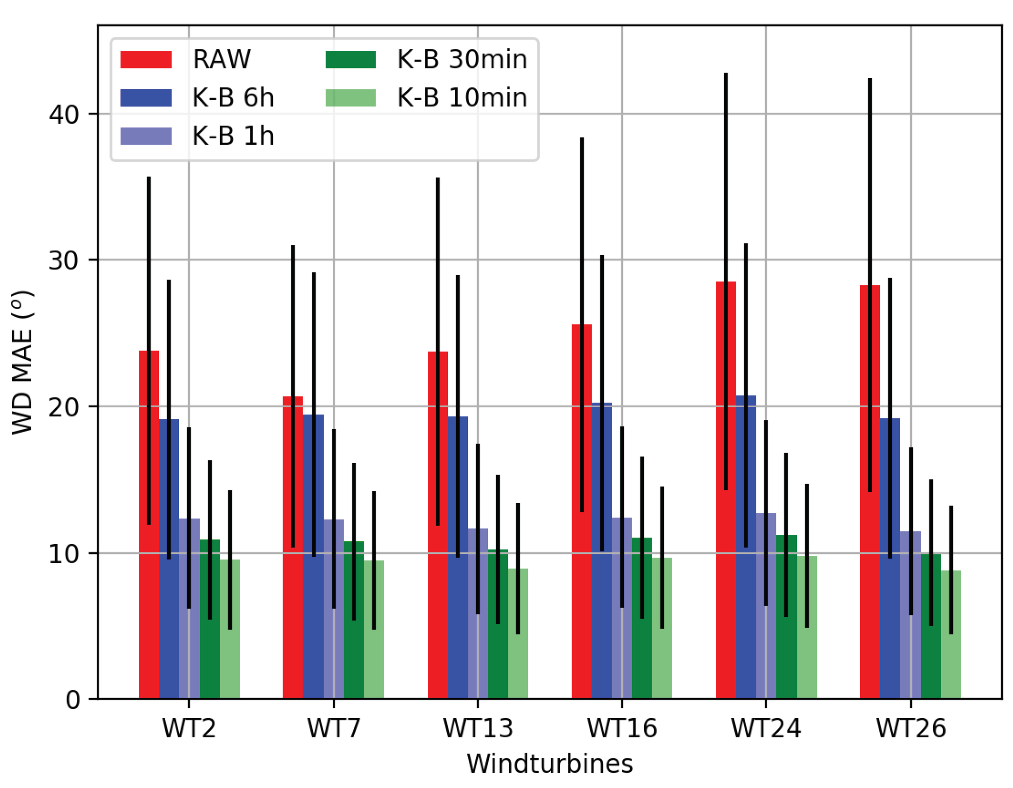
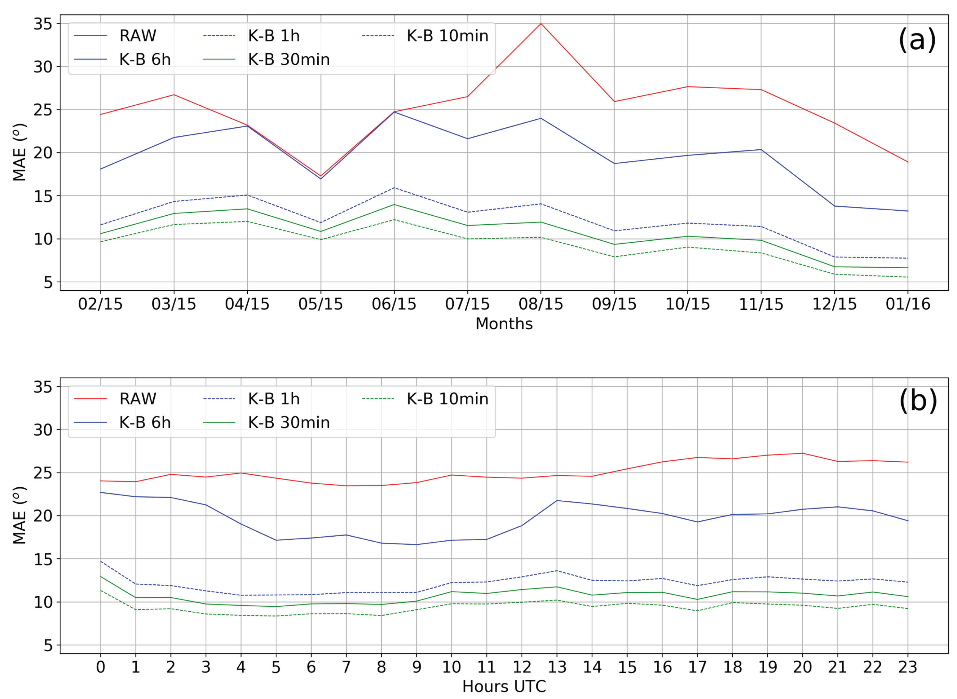
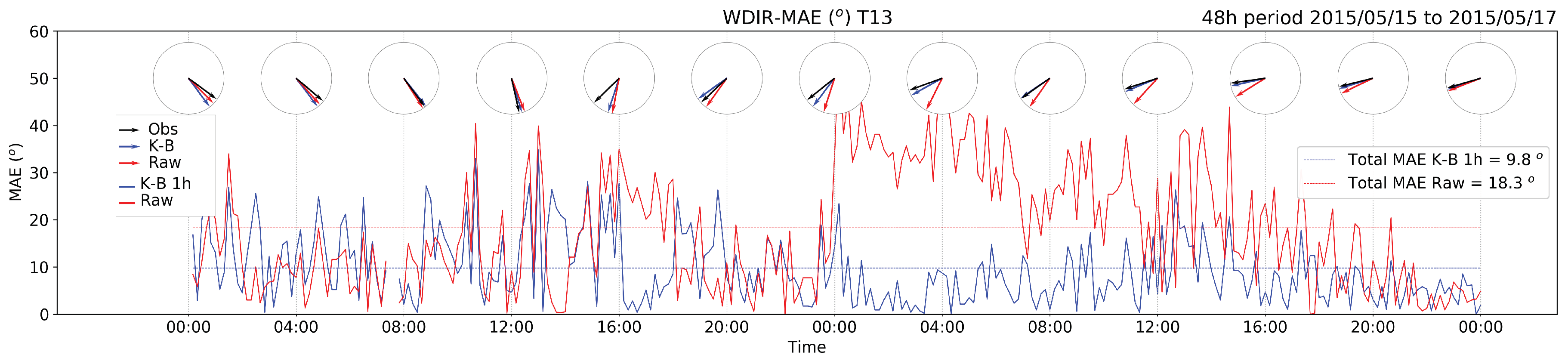
3.2. Wind Direction Nowcasting

Following the discussion on the capabilities of the K-B filter regarding WS (wind speed) nowcasting, we review the statistical tool predicting wind direction (WD) following a similar structure to Section 3.1. To perform the WD nowcasting post-process we obtain the zonal and meridional wind components (U and V) from WS and WD observations, and we use them to correct, with the K-B filter, RAW U and V variables directly extracted from the model output. With the corrected U and V, we recalculate the post-processed WD. Using the same process as in the WS analysis, we test the WD nowcasting for different short-term forecast time periods (Table 2).
Figure 7 displays the annual WD MAE and standard deviation for each turbine and experiment.
The bar chart depicts in red the results of WD MAE for each RAW wind turbine. All of them are above 20 ° ; WT7 with the lowest value, 20.69 ° and WT24 with the highest, 28.51 ° . The mean value of the MAEs for all the wind turbines in the RAW case is 25.10 ° . Comparing K-B 6 h with the unfiltered WRF results, we can see an important amelioration in most of the wind turbines; all of them are now below or practically at 20 ° MAE, reducing the mean total K-B 6 h MAE to 19.67 ° . This value translates into a 22% improvement with respect to RAW results, a correction impact that doubles that obtained in wind speed nowcasting for this same comparison (WS RAW vs. K-B 6 h). This difference can be attributed to the origin of the observational data used. In WS nowcasting we correct one output data series, with another single data series (observed wind speed). However, in WD nowcasting we use WS and WD data from sonic anemometers to obtain the U and V wind components and calculate the post-processed WD. We are thus introducing more sources of error in this last step that the K-B filter seems nevertheless capable of offsetting.
In the shorter lead times of wind direction nowcasting (K-B 1 h, 30 min, and 10 min) the behavior presents a similarity to that of wind speed nowcasting (Figure 2). All the turbines attain analogous error values in each experiment, with a total mean WD MAE of 12.16 ° , 10.69 ° and 9.37 ° for K-B 1 h, K-B 30 min and K-B 10 min respectively. Aside from these low errors, there is also a corresponding reduction of the standard deviation. The K-B filter at short-term nowcasting increases prediction accuracy significantly and eliminates more substantial punctual errors from the original WRF forecasting, which is quite important for the use of these kinds of combined nowcasting systems in wind farm applications. The reason lies in the fact that during daily operations of these installations, wind turbines are continually being orientated depending on wind direction, and potential errors in this manoeuvre lead to machine overstress and production decrease.
As in Section 3.1 for wind speed, the monthly errors for wind direction are shown in Figure 8a, and on a finer timescale, Figure 8b displays the mean hourly wind direction MAE, averaged for all the turbines in the farm. In both cases, RAW WRF outputs are compared with the results of the K-B experiments.
Monthly results in Figure 8a provide insights on the origin of the 22% improvement in forecast skill of K-B 6 h with respect to RAW, commented in Figure 7. From 15 February to 15 March and from 15 July to 16 January, the effect of the K-B 6 h is noticeable, with a decrease in errors of around 7.5 ° during those periods. Nevertheless, the scenario is entirely different in spring, when K-B 6 h practically does not refine the original RAW result. This lack of improvement can be partially explained by the fact that, during spring months, the original WRF outputs register the lowest U and V errors of all the year, and, similarly to previous results, the K-B filter has more difficulties correcting RAW forecast results with low errors.
K-B 1 h, 30 min, and 10 min follow the general tendency of the rest of the comparisons, presenting a substantial error decrease throughout the year. K-B 30 min skill score is always below K-B 1 h and the same for K-B 10 min with respect to K-B 30 min, with all three time series showing a parallel behavior throughout the whole period. As opposed to the case of wind speed (Figure 4), winter months, particularly December and January, have the lowest errors of the series in all wind direction K-B results. For example, K-B 30 min error is around 6.6 ° during these winter months, but over 12 ° in springtime. The lower WD MAE in winter months, on the one hand, seems to be related with the higher mean wind speed registered during that part of the year (Table 3). This means that there are fewer periods of weak winds, which are associated with increased variability in wind direction, presenting, therefore, more difficulties for the K-B filter to handle. On the other hand, these good results during that period can also be related to the clear unimodal wind regime which affects the region during that period.
Changing the timescale of the analysis, Figure 8b shows the evolution of the WD MAE throughout the day. The RAW series (red line) does not present significant hourly changes; all the values are close to 25 ° with a slight increase in the late hours of the day. K-B 6 h differs from this homogeneity, displaying a slight daily cycle with more accurate predictions from 04 to 12 UTC, with a minimum MAE = 16.64 ° at 09 UTC increasing to a maximum of 21.76 ° at 13 UTC. Same as in the daily analysis of wind speed (Figure 5), in the shortest nowcasting periods (1 h, 30 min, and 10 min), the variability is practically eliminated. The K-B filter decreases errors and smooths out the series, with rather constant MAEs around 10 ° throughout the day. The comparisons at different time scales among all the cases confirm that the K-B filter yields a valuable improvement in wind direction prediction. The shortest term nowcasting cases, starting from K-B 1 h, lead to a significant correction of WRF outputs independently of the meteorological situation of the moment.
To conclude this section, in Figure 9 we exemplify the capabilities of wind direction nowcasting with K-B filter. Specifically, a two-day WD MAE comparison is displayed for WT13 between RAW (red) and K-B 1 h (blue). The arrows inside the circles show the instantaneous observed wind direction every four hours (black) and its respective RAW (red) and K-B 1 h (blue) prediction.
The two-day results presented, from 15 May 2015 to 17 May 2015, show different forecast skill patterns. In the first day, RAW and K-B 1 h error series are close to each other in their first 12 h. In the next hours, RAW maintains a more constant higher error (around 25 ° ) for 3–4 h, which K-B 1 h drastically corrects. During the second day, this difference between the time series increases in magnitude; RAW predictions go over MAE = 30 ° for 12 h, reaching up to 40 ° in different moments. Throughout this entire time period, the K-B correction sharply eliminates these big MAEs to values below 10 ° .
Given these results, we can affirm that K-B 1 h provides a good skill improvement in all the situations where the original RAW forecast presents large errors. As in the case of wind speed nowcasting, the correction of big WRF wind direction biases is crucial for wind farm operation applications.

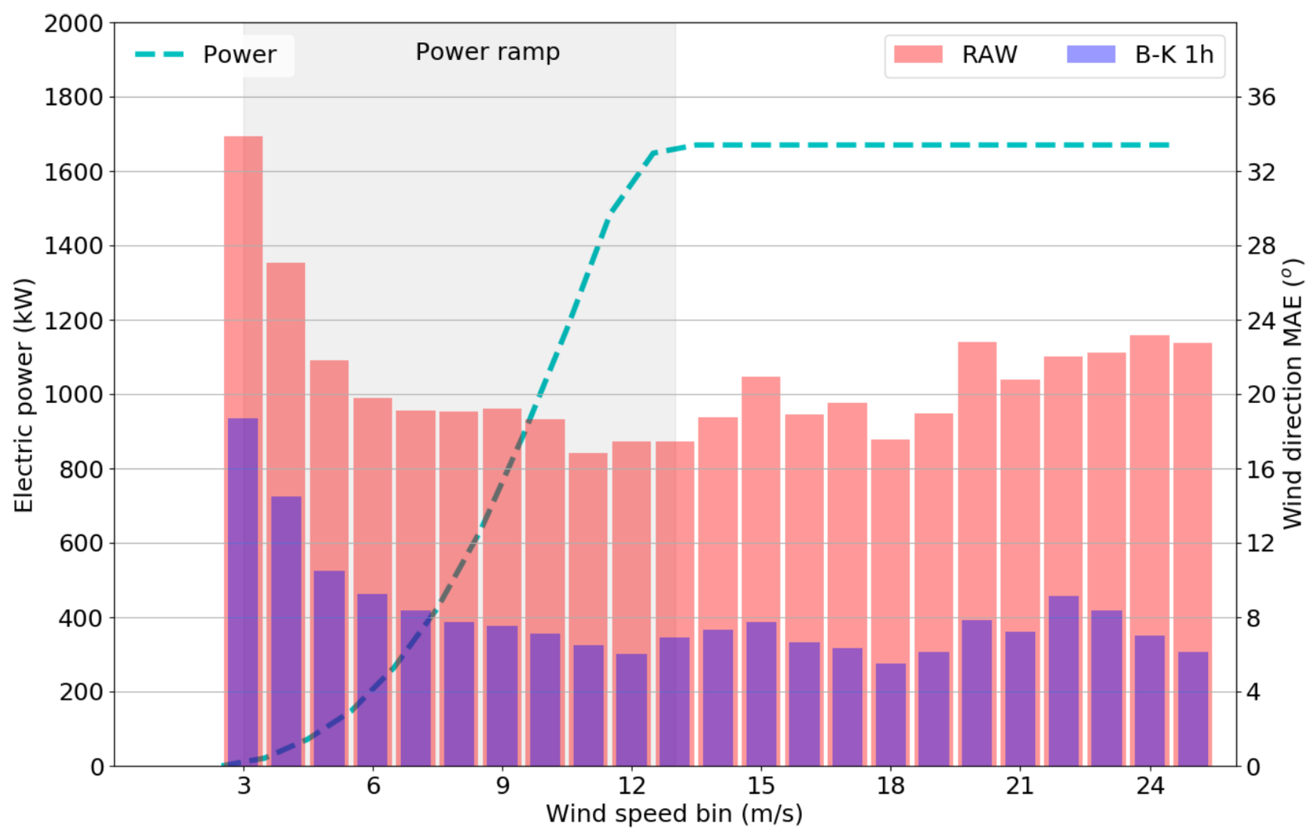
3.3. Application of the K-B Filter for Wind Power Forecasting

In this last section, we test the capabilities of K-B 1 h wind direction nowcasting tool on a real scenario of Coruxeiras wind farm in the studied year, with special attention to critical issues in power prediction, such as wind ramps. For this purpose, we focus on the results corresponding to the wind turbine power ramp, which is the ascending part of the wind power curve before nominal power (Figure 10). Wind speeds within this curve (in this case from 4 to 13 m/s) have the most significant effect in the forecast skill of any nowcasting tool in the wind energy field. In Figure 10, we present the relation between the wind power curve of the wind farm’s turbines (ECOTECNIA74 with 1.670 MW of nominal power [58]) and the WD MAE associated with each wind speed bin, both for RAW and K-B 1 h cases. Table 5 displays the WD MAE in power ramp wind ranges for all the experiments and for each area of the wind farm. It also compares these results with persistence at 10 min, 30 min, and 1 h. The persistence forecast is the assumption that the next timestep value in a prediction is going to be the same as the last measured value [59].
The error bar chart in Figure 10 clearly illustrates the significant improvement of K-B 1 h over RAW results in power ramp winds. At the beginning of the ramp, K-B 1 h obtains a 50% of improvement over RAW. This percentage increases with wind speed, reaching practically a 75% error reduction in the last part of the ramp (12–13 m/s). This is a desirable characteristic of the nowcasting tool because it results in more accurate direction predictions in wind speed situations where energy production values are higher.
Table 5 shows no significant differences among farm areas in power ramp wind direction MAEs. In general, all the experiments achieve better results for power ramp winds than in general for all cases (Figure 7). This is mainly because power ramp situations exclude lower wind occurrences, associated with more variability. Moreover, K-B 1 h and K-B 30 min lead to better results than 1 h and 30 min persistence, respectively. K-B 1 h also reaches lower WD MAE than 30 min persistence.
A K-B nowcasting tool can be useful in the daily management of a wind farm. For instance, an operational K-B 1 h can back up current orientation methods, which are based on SCADA systems [36]. There are also new wind farm control techniques such as yaw-misalignment [60,61], in which upstream wind turbines redirect wakes to increase the production of downstream turbines, that could also benefit from the WRF K-B filter and its capacity to nowcast wind direction with MAEs below 10 ° with a 1 h time horizon.

4. Summary and Conclusions

In the present work, we studied the ability of a new Kalman-Bayesian postprocessing technique to improve the wind speed and wind direction forecasts derived from high-resolution simulations for an operational wind farm over complex terrain. For the needs of the study, a period of one year is simulated utilizing the WRF atmospheric model at a 333 m horizontal resolution, and its outputs post-processed with the K-B filter. We validate the method for different short-term forecast periods, from 6 h to 10 min, with in-situ real data from meteorological stations on the hub of wind turbines.
The results show that the K-B filter in the very short-term (from 1 h to 10 min) is capable of improving the initial wind speed forecasts of the atmospheric model significantly, although the latter are already considerably good (RAW annual WS MAE = 1.87 m/s). The K-B filter achieves a decrease in the WS MAE to 1 m/s for 1 h horizon nowcasting and to 0.72 m/s for the 10 min case. The ME practically disappears when using the K-B 6 h. Analyzing all the experiments in different period ranges (months, hours, instants), we demonstrated that for shorter-term cases, K-B postprocessing eliminates any source of error, improving the prediction in all conditions regardless of the intensity and direction of the wind or the moment of the day and the season of the year.
The effectiveness of the hybrid filter in correcting forecasted wind directions was also a key point of the present study. This was achieved by applying the hybrid post process system to the two-dimensional field of horizontal wind speed components (U and V). The results were quite satisfactory as the K-B 6 h presents a 22% of amelioration with respect to RAW forecasts. Shorter-term cases decrease their WD MAEs even below 10 ° , with an important degree of efficiency in any meteorological situation throughout the year.
It should be noted at this point that several methodologies have been proposed in the literature for the reduction of atmospheric or wave model errors (see for example Landberg and Watson [62] and Joensen et al. [63] for MOS applications, Galanis et al. [23,24]; Kalman [29]; Kalman and Bucy [28]; Kalnay [27]; Louka et al. [34] and Pelland et al. [22] for Kalman filter optimization tools. The proposed methodology in this work that combines Kalman-Bayesin filter applied to single or multiple dimension arrays provides additional advantages and better results in the improvement of wind speed and direction forecasts.
Emphasis was also given to the behavior of wind direction K-B 1 h in power ramp wind cases. The mean results for these are better than for general cases due to the filtering of low winds. K-B 1 h WD improves the persistence forecast for 1 h and 30 min.
In general, the combination of high-resolution WRF simulations and the K-B hybrid filter has shown effectivity and reliability obtaining accurate short-term wind speed and direction predictions, which are of critical importance for an operational wind farm.

Author Contributions

C.O.-C., P.P., G.G. and G.M.-M. designed the research. C.O.-C. and M.A.P. performed the simulations with the WRF model in CESGA computing facilities. P.P. and G.G. implemented the Kalman-Filter tool in the RAW results. C.O.-C., P.P. and M.A.P. analyzed the data. C.O.-C., P.P., G.G. and G.M.-M. drafted the paper. C.O.-C. and M.A.P. designed all the figures. All authors contributed to the interpretation of the data and revision of the paper.

Funding

This research received no external funding.

Acknowledgments

We would like to thank Norvento (http://www.norvento.com/en) for the valuable observational data provided and for their continuing support, both of them were fundamental to accomplishing this project. The model forecast simulations and development of the data analysis were performed at the Centro de Supercomputacion de Galicia (CESGA) (http://www.cesga.es/). Their computer facilities and support have been indispensable during the study.

Conflicts of Interest

The authors declare no conflict of interest.

References

  1. Global Wind Energy Council. Global Wind Report; Technical Report; Global Wind Energy Council: Brussels, Belgium, 2017. [Google Scholar]
  2. Wind Europe. Wind in Power 2017. Annual Combined Onshore and Offshore Wind Energy Statistics; Technical Report; Wind Europe: Brussels, Belgium, 2018. [Google Scholar]
  3. Fried, L.; Shukla, S.; Sawyer, S. Growth Trends and the Future of Wind Energy; Elsevier Inc.: Cambridge, MA, USA, 2017; pp. 559–586. [Google Scholar]
  4. Zhao, J.; Guo, Y.; Xiao, X.; Wang, J.; Chi, D.; Guo, Z. Multi-step wind speed and power forecasts based on a WRF simulation and an optimized association method. Appl. Energy 2017, 197, 183–202. [Google Scholar] [CrossRef]
  5. Prósper, M.A.; Otero-Casal, C.; Fernández, F.C.; Miguez-Macho, G. Wind power forecasting for a real onshore wind farm on complex terrain using WRF high resolution simulations. Renew. Energy 2019, 135, 674–686. [Google Scholar] [CrossRef]
  6. Pokharel, B.; Geerts, B.; Chu, X.; Bergmaier, P. Profiling radar observations and numerical simulations of a downslopewind storm and rotor on the lee of the Medicine Bow mountains in Wyoming. Atmosphere 2017, 8, 39. [Google Scholar] [CrossRef]
  7. Wang, G.M.; Liu, D.F.; Xu, Y.P.; Meng, T.; Zhu, F. PET/CT imaging in diagnosing lymph node metastasis of esophageal carcinoma and its comparison with pathological findings. Eur. Rev. Med. Pharmacol. Sci. 2016, 20, 1495–1500. [Google Scholar] [CrossRef] [PubMed]
  8. Mughal, M.O.; Lynch, M.; Yu, F.; Sutton, J. Forecasting and verification of winds in an East African complex terrain using coupled mesoscale—And micro-scale models. J. Wind Eng. Ind. Aerodyn. 2018, 176, 13–20. [Google Scholar] [CrossRef]
  9. Archer, C.L.; Simão, H.P.; Kempton, W.; Powell, W.B.; Dvorak, M.J. The challenge of integrating offshore wind power in the U.S. electric grid. Part I: Wind forecast error. Renew. Energy 2017, 103, 346–360. [Google Scholar] [CrossRef] [Green Version]
  10. Vanderwende, B.; Lundquist, J.K. Could Crop Height Affect the Wind Resource at Agriculturally Productive Wind Farm Sites? Bound.-Layer Meteorol. 2016, 158, 409–428. [Google Scholar] [CrossRef]
  11. Division, M.; Sciences, O.; Renewable, N. Mesoscale Influences of Wind Farms throughout a Diurnal Cycle. Mon. Weather Rev. 2013, 141, 2173–2198. [Google Scholar] [CrossRef]
  12. Jiménez, P.A.; Navarro, J.; Palomares, A.M.; Dudhia, J. Mesoscale modeling of offshore wind turbine wakes at the wind farm resolving scale: A composite-based analysis with the Weather Research and Forecasting model over Horns Rev. Wind Energy 2015, 18, 559–566. [Google Scholar] [CrossRef]
  13. Muñoz-Esparza, D.; Lundquist, J.K.; Sauer, J.A.; Kosović, B.; Linn, R.R. Coupled mesoscale-LES modeling of a diurnal cycle during the CWEX-13 field campaign: From weather to boundary-layer eddies. J. Adv. Model. Earth Syst. 2017, 9, 1572–1594. [Google Scholar] [CrossRef]
  14. Rai, R.K.; Berg, L.K.; Kosović, B.; Mirocha, J.D.; Pekour, M.S.; Shaw, W.J. Comparison of Measured and Numerically Simulated Turbulence Statistics in a Convective Boundary Layer Over Complex Terrain. Bound.-Layer Meteorol. 2017, 163, 69–89. [Google Scholar] [CrossRef]
  15. Muñoz-Esparza, D.; Kosović, B.; Mirocha, J.; van Beeck, J. Bridging the Transition from Mesoscale to Microscale Turbulence in Numerical Weather Prediction Models. Bound.-Layer Meteorol. 2014, 153, 409–440. [Google Scholar] [CrossRef]
  16. Huang, M.; Wang, Y.; Lou, W.; Cao, S. Multi-scale simulation of time-varying wind fields for Hangzhou Jiubao Bridge during Typhoon Chan-hom. J. Wind Eng. Ind. Aerodyn. 2018, 179, 419–437. [Google Scholar] [CrossRef]
  17. Kariniotakis, G.N.; Pinson, P. Evaluation of the MORE-CARE wind power prediction platform. Performance of the fuzzy logic based models. In Proceedings of the EWEC 2003—European Wind Energy Conference, Madrid, Spain, 16–19 June 2003. [Google Scholar]
  18. Kariniotakis, G.; Martí, I.; Casas, D.; Pinson, P.; Nielsen, T.S.; Madsen, H.; Giebel, G.; Usaola, J.; Sanchez, I. What performance can be expected by short-term wind power prediction models depending on site characteristics? In Proceedings of the EWC 2004 Conference, Tokyo, Japan, 2–4 August 2004; pp. 22–25. [Google Scholar]
  19. Vanem, E. Long-term time-dependent stochastic modelling of extreme waves. Stoch. Environ. Res. Risk Assess. 2011, 25, 185–209. [Google Scholar] [CrossRef]
  20. Giebel, G. On the Benefits of Distributed Generation of Wind Energy in Europe. Ph.D. Thesis, Carl von Ossietzky Universitat Oldenburg, Oldenburg, Germany, August 2001. [Google Scholar]
  21. Resconi, G. Geometry of risk analysis (morphogenetic system). Stoch. Environ. Res. Risk Assess. 2009, 23, 425–432. [Google Scholar] [CrossRef]
  22. Pelland, S.; Galanis, G.; Kallos, G. Solar and photovoltaic forecasting through post-processing of the global environmental multiscale numerical weather prediction model. Prog. Photovolt. Res. Appl. 2011, 21, 284–296. [Google Scholar] [CrossRef]
  23. Galanis, G.; Louka, P.; Katsafados, P.; Pytharoulis, I.; Kallos, G. Applications of Kalman filters based on non-linear functions to numerical weather predictions. Ann. Geophys. 2006, 24, 2451–2460. [Google Scholar] [CrossRef] [Green Version]
  24. Galanis, G.; Emmanouil, G.; Chu, P.C.; Kallos, G. A new methodology for the extension of the impact of data assimilation on ocean wave prediction. Ocean Dyn. 2009, 59, 523–535. [Google Scholar] [CrossRef] [Green Version]
  25. Crochet, P. Adaptive Kalman filtering of 2-metre temperature and 10-metre wind-speed forecasts in Iceland. Meteorol. Appl. 2004, 11, 173–187. [Google Scholar] [CrossRef]
  26. Galanis, G.; Anadranistakis, M. A one-dimensional Kalman filter for the correction of near surface temperature forecasts. Meteorol. Appl. 2002, 9, 437–441. [Google Scholar] [CrossRef] [Green Version]
  27. Kalnay, E. Atmospheric Modeling, Data Assimilation, and Predictability; Cambridge University Press: Cambridge, UK, 2003. [Google Scholar]
  28. Kalman, R.E.; Bucy, R.S. New Results in Linear Filtering and Prediction Theory. J. Basic Eng. 1961, 83, 95. [Google Scholar] [CrossRef]
  29. Kalman, R.E. A New Approach to Linear Filtering and Prediction Problems. J. Basic Eng. 1960, 82, 35. [Google Scholar] [CrossRef]
  30. Stathopoulos, C.; Kaperoni, A.; Galanis, G.; Kallos, G. Wind power prediction based on numerical and statistical models. J. Wind Eng. Ind. Aerodyn. 2013, 112, 25–38. [Google Scholar] [CrossRef]
  31. Hua, S.; Wang, S.; Jin, S.; Feng, S.; Wang, B. Wind speed optimisation method of numerical prediction for wind farm based on Kalman filter method. J. Eng. 2017, 2017, 1146–1149. [Google Scholar] [CrossRef]
  32. Che, Y.; Peng, X.; Monache, L.D.; Kawaguchi, T.; Xiao, F. A wind power forecasting system based on the weather research and forecasting model and Kalman filtering over a wind-farm in Japan. J. Renew. Sustain. Energy 2016, 8, 013302. [Google Scholar] [CrossRef]
  33. Che, Y.; Xiao, F. An integrated wind-forecast system based on the weather research and forecasting model, Kalman filter, and data assimilation with nacelle-wind observation. J. Renew. Sustain. Energy 2016, 8, 053308. [Google Scholar] [CrossRef]
  34. Louka, P.; Galanis, G.; Siebert, N.; Kariniotakis, G.; Katsafados, P.; Pytharoulis, I.; Kallos, G. Improvements in wind speed forecasts for wind power prediction purposes using Kalman filtering. J. Wind Eng. Ind. Aerodyn. 2008, 96, 2348–2362. [Google Scholar] [CrossRef] [Green Version]
  35. Galanis, G.; Papageorgiou, E.; Liakatas, A. A hybrid Bayesian Kalman filter and applications to numerical wind speed modeling. J. Wind Eng. Ind. Aerodyn. 2017, 167, 1–22. [Google Scholar] [CrossRef]
  36. Zaher, A.; McArthur, S.D.; Infield, D.G.; Patel, Y. Online wind turbine fault detection through automated SCADA data analysis. Wind Energy 2009, 12, 574–593. [Google Scholar] [CrossRef]
  37. Drew, D.R.; Cannon, D.J.; Barlow, J.F.; Coker, P.J.; Frame, T.H. The importance of forecasting regional wind power ramping: A case study for the UK. Renew. Energy 2017, 114, 1201–1208. [Google Scholar] [CrossRef] [Green Version]
  38. Lorente-Plazas, R.; Montávez, J.P.; Jimenez, P.A.; Jerez, S.; Gómez-Navarro, J.J.; García-Valero, J.A.; Jimenez-Guerrero, P. Characterization of surface winds over the Iberian Peninsula. Int. J. Climatol. 2015, 35, 1007–1026. [Google Scholar] [CrossRef]
  39. Santos, J.A.; Rochinha, C.; Liberato, M.L.; Reyers, M.; Pinto, J.G. Projected changes in wind energy potentials over Iberia. Renew. Energy 2015, 75, 68–80. [Google Scholar] [CrossRef]
  40. Skamarock, W.; Klemp, J.; Dudhi, J.; Gill, D.; Barker, D.; Duda, M.; Huang, X.Y.; Wang, W.; Powers, J. A Description of the Advanced Research WRF Version 3; Technical Report; NCAR: Boulder, CO, USA, 2008. [Google Scholar]
  41. Wang, W.; Bruyère, C.; Duda, M.; Dudhia, J.; Gill, D.; Kavulich, M.; Keene, K.; Lin, H.C.; Michalakes, J.; Rizvi, S.; et al. ARW Version 3 Modeling System User’s Guide. J. Palest. Stud. 2007, 37, 204–205. [Google Scholar] [CrossRef]
  42. Shin, H.H.; Hong, S.Y.; Dudhia, J. Impacts of the Lowest Model Level Height on the Performance of Planetary Boundary Layer Parameterizations. Mon. Weather Rev. 2012, 140, 664–682. [Google Scholar] [CrossRef]
  43. Slater, J.A.; Heady, B.; Kroenung, G.; Curtis, W.; Haase, J.; Hoegemann, D.; Shockley, C.; Tracy, K. Evaluation of the New ASTER Global Digital Elevation Model; National Geospatial-Intelligence Agency: Reston, VA, USA, 2009; pp. 335–349.
  44. European Environment Agency. CLC2006 Technical Guidelines; European Environment Agency: Copenhagen, Denmark, 2007; Volume 2010, p. 70. [CrossRef]
  45. Hong, S.; Lim, J. The WRF single-moment 6-class microphysics scheme (WSM6). Asia-Pac. J. Atmos. Sci. 2006, 42, 129–151. [Google Scholar]
  46. Kain, J.S. The Kain–Fritsch Convective Parameterization: An Update. J. Appl. Meteorol. 2004, 43, 170–181. [Google Scholar] [CrossRef]
  47. Mlawer, E.J.; Taubman, S.J.; Brown, P.D.; Iacono, M.J.; Clough, S.A. Radiative transfer for inhomogeneous atmospheres: RRTM, a validated correlated-k model for the longwave. J. Geophys. Res. Atmos. 1997, 102, 16663–16682. [Google Scholar] [CrossRef] [Green Version]
  48. Dudhia, J. Numerical Study of Convection Observed during the Winter Monsoon Experiment Using a Mesoscale Two-Dimensional Model. J. Atmos. Sci. 1989, 46, 3077–3107. [Google Scholar] [CrossRef]
  49. Nakanishi, M.; Niino, H. An improved Mellor-Yamada Level-3 model: Its numerical stability and application to a regional prediction of advection fog. Bound.-Layer Meteorol. 2006, 119, 397–407. [Google Scholar] [CrossRef]
  50. Beljaars, A.C. The parametrization of surface fluxes in large-scale models under free convection. Q. J. R. Meteorol. Soc. 1995, 121, 255–270. [Google Scholar] [CrossRef]
  51. Tewari, M.; Chen, F.; Wang, W.; Dudhia, J.; Lemone, M.A.; Mitchell, K.; Cuenca, R.H.; Springs, C.; Force, A.; Agency, W. Implementation and Verification of The Unified NOAH Land Surface Model In The WRF Model. In Proceedings of the 20th Conference on Weather Analysis and Forecasting/16th Conference on Numerical Weather Prediction, Seattle, WA, USA, 12–16 January 2004. [Google Scholar]
  52. Fitch, A.C.; Olson, J.B.; Lundquist, J.K.; Dudhia, J.; Gupta, A.K.; Michalakes, J.; Barstad, I. Local and Mesoscale Impacts of Wind Farms as Parameterized in a Mesoscale NWP Model. Mon. Weather Rev. 2012, 140, 3017–3038. [Google Scholar] [CrossRef]
  53. Patlakas, P.; Drakaki, E.; Galanis, G.; Spyrou, C.; Kallos, G. Wind gust estimation by combining a numerical weather prediction model and statistical post-processing. Energy Procedia 2017, 125, 190–198. [Google Scholar] [CrossRef]
  54. BOX CEP; Tiao, G.C. Bayesian Inference in Statistical Analysis; Wiley: Hoboken, NJ, USA, 1992. [Google Scholar] [CrossRef]
  55. Bernardo, J.; Smith, A. Bayesian Theory; Wiley: Hoboken, NJ, USA, 2000. [Google Scholar]
  56. Kuikka, I. Wind Nowcasting: Optimizing Runway in Use; Technical Report; Helsinki University of Technology Systems Analysis Laboratory: Espoo, Finland, 2009. [Google Scholar]
  57. Gupta, H.V.; Sorooshian, S.; Yapo, P.O. Status of automatic calibration for hydrologic models: Comparison with multilevel expert calibration. J. Hydrol. Eng. 1999, 4, 135–143. [Google Scholar] [CrossRef]
  58. Ecotèctnia. Technical Report 74 1.6; Technical Report; ECOTÈCNIA: Barcelona, Spain, 2007. [Google Scholar]
  59. Utsumi, H.; Misaka, T.; Moteki, W. Prediction Model of Internal Relative Humidity During Self-desiccation in Hardened Cement Pastes. Concr. Res. Technol. 2015, 26, 11–19. [Google Scholar] [CrossRef] [Green Version]
  60. Van Dijk, M.T.; Van Wingerden, J.W.; Ashuri, T.; Li, Y.; Rotea, M.A. Yaw-Misalignment and its Impact on Wind Turbine Loads and Wind Farm Power Output. J. Phys. Conf. Ser. 2016, 753, 062013. [Google Scholar] [CrossRef]
  61. Churchfield, M.; Fleming, P. Wind Turbine Wake-Redirection Control at the Fishermen’s Atlantic City Windfarm. Offshore Technol. 2015. [Google Scholar] [CrossRef]
  62. Landberg, L.; Watson, S.J. Short-term prediction of local wind conditions. Bound.-Layer Meteorol. 1994, 70, 171–195. [Google Scholar] [CrossRef]
  63. Joensen, A.; Giebel, G.; Landberg, L.; Madsen, H.; Neilsen, H. Model output statistics applied to wind power prediction. In Proceedings of the EWEC-Conference, Nice, France, 1–5 March 1999; pp. 1177–1180. [Google Scholar]
Figure 1. (a) WRF nested grid configuration, with the number of points for each domain indicated. (b) D04 is expanded showing its topography. Coruxeiras wind farm is located in the central area of D04, on top of a hill. Observational data for the study is obtained from meteorological stations at the hub of the wind turbines plotted in red. (c) Annual wind rose from observational data at hub height from a wind turbine in the center of the farm (WT13).
Energies 12 03050 g001
Figure 2. Barchart with annual WS MAE for all experiments and wind turbines analyzed. For each case, the standard deviation ( σ ) is represented by a black line on top of each bar.
Energies 12 03050 g002
Figure 3. (a) Wind speed distribution plot for observations, RAW, K-B 6 h and K-B 1 h time experiments in the north area of the wind farm. The standard deviation of each distribution is indicated in the legend. (b) Radar charts comparing WS errors by observed wind direction in the north area. (c) Same as (a) for the center area. (d) Same as (b) for the center area. (e) Same as (a) for the south area. (f) Same as (b) for the southern area.
Energies 12 03050 g003
Figure 4. Monthly wind speed MAE for the wind turbines with K-B model (6 h (blue), 1 h (dotted blue), 30 min (green), and 10 min (dotted green)) and RAW (red).
Energies 12 03050 g004
Figure 5. Wind speed MAE for all the turbines, hourly (moving average) for the entire 24 h simulation period with RAW outputs (red) and K-B model cases: K-B 6 h (blue), K-B 1 h (dotted blue), K-B 30 min (green) and K-B 10 min (dotted green).
Energies 12 03050 g005
Figure 6. (a) Wind speed at hub height in the center area with observations (orange), RAW (dotted red), and K-B 1 h (blue) in May. (b) Same as (a) in December. Wind speed MAE, PBIAS and Correlation Coefficient (CC) for each series is presented in the legend for both figures.
Energies 12 03050 g006
Figure 7. Barchart with annual WD MAE for all experiments and wind turbines analyzed. For each case, the standard deviation is represented by a black line ( σ ) on top of each bar.
Energies 12 03050 g007
Figure 8. (a) Monthly wind direction MAE for the wind farm with K-B model experiments and RAW. (b) Wind direction MAE, hourly (moving average) for the entire 24 h simulation period. In both cases the comparison is between RAW outputs (red) and K-B model cases: K-B 6 h (blue), K-B 1 h (dotted blue), K-B 30 min (green) and K-B 10 min (dotted green).
Energies 12 03050 g008
Figure 9. Wind direction MAE with K-B 1 h filter and RAW in W13 during a 48 h period. Wind direction arrows with observations, K-B 1 h, and RAW are displayed on top every four hours.
Energies 12 03050 g009
Figure 10. ECOTECNIA 74 wind power curve (density = 1.112 kg/m 3 , height = 975 m, temperature = 9 ° C), cyan line. Each bar of the figure represents the wind direction MAE associated with wind speed bins with a bandwidth of 1 m/s both for RAW (red) and K-B 1 h (blue).
Energies 12 03050 g010
Table 1. The principal physical schemes used in the atmospheric model.
MicrophysicsSingle-moment six-class scheme [45]
Cumulus ParameterizationKain-Fritsch scheme [46] disabled in d04 and d05
Long wave radiation physicsRRTM Longwave model [47]
Short wave radiation physicsDudhia shortwave radiation schemes [48]
Planetary boundary layerMellor–Yamada Nakanishi Niino Level 2.5 [49]
Surface layer optionRevised MM5 Monin-Obukhov scheme [50]
Land-surface physicsNoah land-surface model [51]
Wind Turbine ParameterizationFitch, A. C. 2012 [11]
Table 2. Short explanation of the experiments tested in this study. The bold names on the left are the identifiers used hereafter for each case.
ExperimentDescription
RAWWRF results without post-proccess
K-B 6 hK-B filter nowcasting used for 6 h time horizon
K-B 1 hK-B filter nowcasting used for 1 h time horizon
K-B 30 minK-B filter nowcasting used for 30 min time horizon
K-B 10 minK-B filter nowcasting used for 10 min time horizon
Table 3. WS ME and WS RMSE for all experiments and wind turbines.
(a) WS ME (m/s)
RAWK-B 6 hK-B 1 hK-B 30 minK-B 10 min
WT2−0.4190.0260.0170.0090.004
WT7−0.4460.0110.0160.0090.004
WT13−0.3310.1020.0140.0080.006
WT16−0.5900.0690.0250.0130.006
WT24−0.4490.0190.0210.0130.006
WT26−1.4000.0480.0220.0120.004
TOTAL−0.6050.0460.0190.0110.005
(b) WS RMSE (m/s)
RAWK-B 6 hK-B 1 hK-B 30 minK-B 10 min
WT22.4262.3761.4111.1940.986
WT72.5082.3251.4131.1990.990
WT132.5282.4981.4451.2191.001
WT162.4252.3221.4351.2261.019
WT242.3272.1891.3701.1700.969
WT263.0092.4491.4641.2371.022
TOTAL2.5372.3591.4231.2070.998
Table 4. Observed mean monthly wind speed normalized with observed mean annual wind speed.
Mean Monthly WS /Mean Annual WS
JanuaryFebruaryMarchAprilMayJuneJulyAugustSeptemberOctoberNovemberDecember
1.41.160.970.851.070.770.80.760.831.020.881.48
Table 5. WD MAE for all the experiments and different persistence periods in power ramp winds.
Power Ramp Winds (49.7%)
Wind Dir. MAE ( ° )
NorthCenterSouthTotal
Per. 10 min6.546.326.966.61
Per. 30 min8.498.318.848.55
Per. 1 h10.079.9210.4710.15
K-B 10 min6.656.526.916.70
K-B 30 min7.457.357.717.51
K-B 1 h8.338.268.568.38
K-B 6 h13.5913.7114.1013.80
RAW16.0719.5422.8119.47

