Abstract
The estimation of solar radiation for planning current and future periods in different fields, such as renewable energy generation, is very important for decision makers. The current study presents a hybrid model structure based on a multi-objective shark algorithm and fuzzy method for forecasting and generating a zone map for solar radiation as an alternative solution for future renewable energy production. The multi-objective shark algorithm attempts to select the best input combination for solar radiation (SR) estimation and the optimal value of the adaptive neuro-fuzzy inference system (ANFIS) parameter, and the power parameter of the inverse distance weight (IDW) is computed. Three provinces in Iran with different climates and air quality index conditions have been considered as case studies for this research. In addition, comparative analysis has been carried out with other models, including multi-objective genetic algorithm-ANFIS and multi-objective particle swarm optimization-ANFIS. The Taguchi model is used to obtain the best value of random parameters for multi-objective algorithms. The comparison of the results shows that the relative deviation index (RDI) of the distributed solutions in the Pareto front based multi-objective shark algorithm has the lowest value in the spread index, spacing metric index, favorable distribution, and good diversity. The generated Pareto solutions based on the multi-objective shark algorithm are compared to those based on the genetic algorithm and particle swarm algorithm and found to be the optimal and near ideal solutions. In addition, the determination of the best solution based on a multi-criteria decision model enables the best input to the model to be selected based on different effective parameters. Three different performance indices have been used in this study, including the root mean square error, Nash–Sutcliffe efficiency, and mean absolute error. The generated zone map based on the multi-objective shark algorithm-ANFIS highly matches with the observed data in all zones in all case studies. Additionally, the analysis shows that the air quality index (AQI) should be considered as effective input for SR estimation. Finally, the measurement and analysis of the uncertainty based on the multi-objective shark algorithm-ANFIS were carried out. As a result, the proposed new hybrid model is highly suitable for the generation of accurate zone mapping for different renewable energy generation fields. In addition, the proposed hybrid model showed outstanding performance for the development of a forecasting model for the solar radiation value, which is essential for the decision-makers to draw a future plan for generating renewable energy based solar radiation.
1. Introduction
The Sun is considered a fundamental resource for most physical and chemical processes on Earth. Thus, processes related to the Sun are important for researchers [1,2]. The application of solar energy for different aims as a renewable energy source is an important priority for researchers [3]. Renewable energy technologies are fast becoming more effective and cheaper and their application is widely growing. Solar radiation is one of the most important resources of renewable energy [4]. In fact, the wide application of solar energy as renewable energy can decrease greenhouse emissions. Renewable energy, such as solar radiation, has a low effect on the environment. In this context, decision makers should know the available solar radiation in order to be able to identify the expected generation of renewable energy. Therefore, the development of an accurate forecasting model and generation of zone mapping for solar radiation is of vital importance for decision-makers. In addition, with the world becoming warmer, renewable energies can balance the ecological conditions and the production of domestic power can be carried out based on the use of solar energy [5,6].
In fact, Solar Radiation (SR) affects climate processes, and agricultural production is governed by solar energy [7]. SR is necessary for plant growth, photosynthesis, and regulation of the growth duration. The estimation of SR has many applications in different fields, including agricultural engineering, building engineering, the energy and hydrology fields, and power and heat production [8]. For example, the accurate estimation of irrigation is considered an important issue for irrigation planning and design [9]. Additionally, SR is considered an important issue for evaporation computation [10]. Thus, access to solar data and an accurate model for the prediction of SR data are important for the leverage of the solar energy potential in particular locations. There are different empirical models and equations for SR estimation. These models are highly important because of the economic limitation and measurement complexity of SR estimation in some locations, rendering empirical models suitable for radiation estimation [11]. Additionally, remote sensing and satellite images can be considered effective tools for solar energy estimation. However, these empirical models require various parameters that might be too complex to be accurately estimated in some locations. In addition, some models cannot provide a good estimation of SR under changing climate conditions and other conditions [12]. The station height from sea level, longitude, latitude, relative humidity, and pollution accumulation in the atmosphere affect radiation estimations. Thus, the pollution content is an important and influential issue affecting SR, and the application of accurate tools for radiation estimation under the effect of different parameters is very important for decision makers [13]. Soft computing methods can be effective as powerful tools based on large data sets because these methods can accurately simulate hydrological or other variables. These methods can effectively adapt to climate and hydrological boundaries, decrease the computational time, and ensure high accuracy in hydrological predictions [14]. In addition, soft computing methods can be effective tools for estimating SR when different parameters, such as particle pollution, temperature, humidity, etc., have a significant effect on SR [15]. The present study attempts to simulate the SR in East Azarbayejan in Iran in some stations in the presence of particle pollution. The current article presents self-organizing maps (SOMs) with a multi-objective shark algorithm (MOSA), and the fuzzy method is applied to select the optimal input combinations, identify the best value of the ANFIS parameters, and generate the spatial distribution of SR. The SOM is used as a clustering method to identify impactful spatial SR values, and the results are compared with those obtained using the multi-objective genetic algorithm (MOGA) and multi-objective particle swarm optimization (MPSO).
2. Background
An ANN model based on different numbers of inputs in different cities in Turkey was previously used to simulate SR [16]. The results indicated that using a pre-selection procedure is necessary for the determination of the inputs because the elimination of some input parameters could significantly decrease the accuracy of the models. The ANN used for different climate change conditions had acceptable performance for SR based on the accuracy of the parameter selection.
Another study simulated the monthly and daily total global SR based on an artificial neural network (ANN) [17]. The soil temperature, wind speed, temperature, and mean monthly rainfall were used to estimate SR. The results indicated that the mean absolute percentage error (MAPE) based on the ANN was approximately 5.34% and that the ANN method decreased the MAPE compared with the output of the regression method with a high correlation.
The auto regressive moving average mode (ARMA) and multi-layer perceptron (MLP) have been used as hybrid models to simulate hourly SR [18]. The results indicated that the hybrid model had a lower root mean square error (RMSE) than the simple MLP model, and the necessary data for this research were obtained based on a numerical weather simulation model.
A regression model was used to estimate hourly SR values [19]. The relative humidity, atmospheric pressure, air pollution index, and mean rainfall were used as inputs in the models. The results indicated that the models incorporating the air pollution index could produce a relatively accurate estimate of SR with a high Nash–Sutcliffe efficiency value and a small RMSE value.
The daily SR has also been predicted by a support vector machine (SVM) [20]. The SVM method was used based on the sunshine ratio as an effective input, and the results were compared with those obtained using empirical models. Compared to the empirical models, the SVM models could significantly reduce the relative error and provide more accurate predictions of the winter season.
Vakili et al. [21] simulated the daily SR based on an ANN while considering the suspended particulate matter. The temperature, rainfall, humidity, and suspended particle characteristics were used to simulate SR in Tehran Province, Iran, and the results indicated that compared to the other applied methods’ input structure, the ANN considering the suspended particles could simulate SR with the lowest error in terms of the RMSE and mean absolute error.
The hourly global horizontal irradiance (HGI) was estimated based on Meteosat imagery and an ANN [22]. The data were obtained from a radiometric station. The Heliosat-2 model was used to compare the results with those obtained using an ANN. The results obtained by the ANN based on different sky conditions had a significantly lower RMSE value than those obtained by the Heliosat-2 model.
Celik et al. [23] applied an optimized ANN for SR estimation over the Eastern Mediterranean. The results indicated that the daily SR could be predicted based on the optimized ANN with high accuracy such that the optimized model could accurately determine the number of hidden neurons and weights in the ANN, and the RMSE was decreased by approximately 10% to 12% compared to that obtained using regression methods.
A moderate-resolution imaging spectroradiometer (MODIS) and an ANN have also been used to obtain SR estimates [24]. Land surface temperature (LST) data were used as input data to the ANN, and the results indicated that the relative error of the ANN was 5.35%, while the error of the regression models was 10.23%.
The new daily SR model (NDSRM) using the air quality index (AQI) was applied in multiple cities [25]. The results differed according to whether the AQI was added or removed from the inputs such that the predicted SR based on the elimination of the AQI in some cities had high accuracy, whereas the model accuracy depended on the AQI value as input in other cities.
The ANN model and inverse distance weight (IDW)-based model were used to simulate SR at distances greater than 50 km [26]. The results indicated that the IDW model had an RMSE of approximately 6.4%, while the RMSE of the ANN model was 5.11%, and the IDW model was simpler and more accurate than the ANN model.
Yoe et al. [25] applied the SVM to SR estimation based on the air quality index. The results indicated that the Nash–Sutcliffe efficiency varied from 0.682 to 0.740, and the models with the AQI input provided a higher accuracy in solar estimation than those without this input.
The daily SR considering the air quality index was simulated by a support vector machine (SVM) in a large region with different climates [2]. The results indicated that the elimination of the AQI input among the other inputs could significantly decrease the accuracy of the estimation model; the SVM featured a high accuracy, and simple structures were found to have a high ability to absorb SR.
Fan et al. [27] applied an SVM for SR estimation while considering atmospheric particulate matter (PM). Daily metrological and air pollution data were used to simulate SR. The inclusion of PM with a diameter of 2.5 micrometres (PM 2.5), PM 10, and O3 in the input combinations were considered the best combination of inputs and improved the results of the SVM.
Furthermore, many research efforts have attempted to simulate SR based on soft computing methods under different conditions, such as using air pollution data. Different air quality indexes have been used to evaluate the air quality, such as the air pollution index (API) and air quality index (AQI) [28]. The AQI is used to provide a daily evaluation of the air quality. This index is used to present the air quality to the population while focusing on the respiratory effects that can be observed some hours or days after exposure [29]. The AQI is computed based on models or air monitors considering nitrogen dioxide, ozone, carbon monoxide, and sulfur dioxide [30]. This index ranges from 0 to 500, which is divided into different classifications, and each classification is related to different levels of human health. The country of Iran experiences considerable air pollution in different cities; this air pollution is usually measured and evaluated with the index, and the classification changes accordingly [31]. For example, when the index value is within the range of 0 to 50, the air quality is good, and when the index value is greater than 300, the air quality is very dangerous. A literature review of the pollutant particle effect on SR shows that several studies have considered the effect of air quality on SR [31].
Thus, the main purpose of the current paper is to evaluate the effect of air quality on SR using soft computing models to provide a comprehensive discussion concerning the influences of the air quality on the accuracy of SR prediction. In this study, the ANFIS model was selected as the soft computing method because ANFIS is suitable for predicting stochastic nature variables, such as SR. However, in the ANFIS model procedure, there is a need to initialize a few internal parameters that are usually selected using the trial-and-error process. The selection of the optimal values of these parameters significantly affects the accuracy of the model performance. In this context, there is a need to optimize the value of the ANFIS’s internal parameter to ensure an acceptable level of prediction accuracy. In fact, the shark algorithm is widely accepted and has been successfully applied in the fields of water resources and power generation, mathematical simulations, the design of trusses, and other fields [32,33]. Therefore, the shark algorithm is used as an effective optimization tool to obtain the optimal parameters for the ANFIS. The rotational movement of the shark in this algorithm improves the ability to search for the global optima of the ANFIS’s internal parameters. The proposed integrated adaptive neuro-fuzzy inference system with multi-objective shark algorithm (ANFIS-MOSA) model was examined in SR prediction in three different case studies. In addition, comprehensive analyses were carried out to compare the proposed model to other models.
3. Materials and Methods
3.1. Fuzzy Method
The ANFIS model, which is based on large amounts of data, can accurately simulate different variables, such as hydrological parameters, water quality parameters, climate parameters, and other parameters. The following six layers are used in the ANFIS:
- The first layer with inputs x and y is connected to the neurons in the adjacent layer.
- The nodes in layer 2 constitute the fuzzification layer, and this layer includes an adaptive node that has a function. The fuzzy membership function is computed in this layer as follows:
There are different types of membership functions, and the following bell function has been widely used with successful applications in previous research:
where , , and ci are premise parameters that can be obtained based on the optimization process.
- The firing strength (wi) is computed in the third layer as follows:
Each node in the fourth layer computes the ratio of the firing strength of the membership rules to the firing strength of the total number of rules. The output is computed based on the following equation:
- Each node in the fifth layer is considered an adaptive square node with a node function:where pi, qi, and ri are considered the consequent parameters.
- The overall output in the sixth layer is computed based on signals received from the defuzzification layer and the following equation:
However, the consequent parameters and premise parameters should be determined accurately, and an optimization algorithm can obtain the accurate value of these parameters if the initial estimates of the parameter values are inserted into the algorithms as decision variables.
3.2. Shark Algorithm (SA)
The shark algorithm acts based on smell receptors in idealized sharks. The algorithm, which features a simple structure, high flexibility, resistance to trapping in local optima, and fast convergence, has been successfully applied in the fields of water resource management, reservoir operation, and power generation. The initial positions of the sharks are considered decision variables based on the following equation [34]:
where is the jth dimension of the ith shark position, ND is the number of decision variables, and is the initial shark position. The SA has the following three main assumptions:
- The injured fish are considered prey to the sharks, and the movement velocity of the fish is very low compared to the shark velocity due to their injuries. The sharks find the fish locations by detecting blood from the injured fish.
- Blood is regularly emitted from the fish bodies, and the water flow has a negligible effect on the blood emission and movement in the water. When the number of blood particles around the injured fish is considerable, the smell receptors of the shark can detect the blood odor, and the shark moves to the location of the fish.
- Each injured fish is considered one blood source.
Sharks moving in water have a specific velocity [34] as follows:
where is the jth dimension of the ith velocity position, ND is the number of decision variables, and is the initial shark velocity.
The shark velocity varies based on the detected smell intensity, and when sharks detect a higher odor concentration, they rapidly move in the direction of the target. If the variation in the odor concentrations is considered a gradient of the objective function, the velocity varies according to the gradient of the objective function based on the following equation:
where is the objective function, k is the stage number, NP is the population size, is a random value between 0 and 1, and is a random value. The forward movement of the sharks is based on the k number stage such that the maximum number stage equals kmax. The sharks are subjected to an inertial limitation, and thus, they move at a specific velocity as follows:
where is a momentum coefficient between 0 and 1, and is a random value. A momentum rate with a higher value indicates greater inertia, and thus, the current velocity strongly depends on the previous velocity. The normal velocity of a shark is 20 km/hr, and the maximum velocity of a shark is 80 km/hr; thus, there is a limitation to the velocity based on the following equation:
where is the velocity limiter. The new shark position is computed based on the following equation:
where is the new shark position, and is the time interval. The rotational movement of the shark is considered a local search to find the best solution based on the following equation:
where R3 is a random number, M is the total number of points in the local search and rotational point, and m is the number of each rotation level. In fact, there are M points around ; thus, the sharks manifest rotational movement around these points. Then, the sharks select the best position based on the obtained positions and positions.
3.3. Multi-Objective Algorithms
An optimization problem can have one or more objective functions. The framework of a multi-objective function can be defined based on the following equation [35]:
where is the solution vector, fj is the jth objective function, m is the number of objective functions, l is the number of constraints, and are the upper and lower constraints, respectively, and gl and bl are the ith constraints related to the right-hand side.
When the problem has one objective function, the solutions based on different methods can be easily compared, but the domination concept should be used when two objective functions can be identified for the problem. The solution, , dominates the solution, , if the following is satisfied with the problem:
The Pareto front includes solutions such that any other solution cannot dominate the Pareto set in the problem space. The optimal Pareto front is used to define the objective function values based on the following equation:
The main aim of the problem is related to identifying the Pareto front with the highest diversity. A set of non-dominated solutions for the multi-objective problem is selected, and the decision maker selects one solution as the best solution based on an accurate evaluation.
3.4. Multi-Objective Shark Algorithm (MOSA)
The shark positions in the MOSA are considered solutions to the problem, and these positions are generated randomly at the initial level of the MOSA. The non-dominated solutions are saved in an archive and generate a POF. Then, the equality of the solutions is investigated based on a computation of the objective function. The non-dominated sharks in the new archive are computed and recorded in an archive. The following aspects of the archive should be considered:
- If the new solution is dominated by at least one current solution in the archive, the new solution is not inserted into the archive.
- If the new solution dominates over older solutions, the non-dominated solutions are eliminated, and the new solution is inserted into the archive.
- If no new solutions or current solutions in the archive can dominate each other, the new solutions are added to the archive.
Several hypercubes are produced by dividing the objective function spaces by a grid-based mechanism. When the archive size exceeds the capacity, additional sharks should be eliminated from the archive. Hypercubes with a relatively low density are important for the generation of a uniform distribution, and elimination can occur in areas with greater hypercube crowding.
3.5. Non-Dominated Sorting Genetic Algorithm (NSGA)
was generated by Deb [36]. A random population based on generation chromosomes is considered in the first level of . The children chromosomes are generated based on crossover and mutation operators, and their objective function is computed. Then, the combination of the parent and children populations is divided over the fronts based on non-dominated sorting as described by Deb [36]. The crowding distance of each member is computed, and the population is sorted based on this index. Then, the combined population after the sorting mechanism is truncated, such as the parent population, and a new population is prepared to produce a child population. After a ranking process, the first-ranked solution represents the best solution.
3.6. Multi-Objective Particle Swarm Optimization (MPSO)
If the problem space is considered with d dimensions and particles, the ith position particle at the ith position, , has a velocity of . The best performance of each particle in the swarm is [37]. Each particle attempts to improve its position, velocity, and distance with respect to the best particle. The position and velocity of the particles are updated based on the following equations:
where is the inertia coefficient, is the global best output of the particle, is the personal best output of the particle, is the cognitive acceleration coefficient, is the social acceleration coefficient, are random numbers, is the velocity at time t + 1, and is the position at time t + 1.
The MPSO algorithm encounters a set of solutions as a Pareto front [38]. The archive of a non-dominated solution is considered in the solutions developed at each level. First, the initial position and velocity of the particles are considered in the MPSO, and their objective function is computed [39]. Then, the leader is selected from the archive as the particle with the best objective function value such that each particle follows one leader in the archive, and the velocity and position of each particle are updated. The objective function of the new positions and velocities is computed. If the new solution can dominate over , the new solution is inserted into the archive instead of . An efficient mutation strategy for increasing diversity can be considered at this level and applied to the particles. One of the objective functions is selected for the level mutation, and then, the particles are sorted in descending order at this level based on the objective function computation. The crowding distance of the particles in the archive is computed, and sorting is performed in descending order. Then, elitist mutation is applied to a predefined number of available solutions in the archives. The convergence criteria are checked, and if the criteria are not satisfied, the system returns to updating the velocity and position and determining whether the algorithm has completed.
4. Case Study
The current study considers SR over Ardebil, Gilan, and East Azarbayejan. East Azarbayejan has an area of approximately 47,830 km2 (Figure 1). The northern extent of East Azarbayejan is a part of the Republic of Azarbayejan and Armenia. Zanjan Province is located in the south of this province, and the Sahand Mountain, which has a height of 3707 m, is one of the highest points in the province. The annual temperature from 2008 to 2018 ranged between 25 and −15 °C. This province is located between the longitudes of 45°0′ E and 47°50′ E and latitudes of 36°50′ to 39°50′. This province is mountainous as follows: 40% of the province area has mountainous conditions. The climate in this province is cold and dry, but the different topographies cause variations in the climates. The maximum temperature, precipitation, and number of sunny hours obtained from three stations, i.e., Ahar (longitude: 47°48′ and latitude: 38°28′), Bonab (longitude: 45°70′ and latitude: 37°20′), and Sarab (longitude: 47°23′ and latitude: 37°51′), were considered. Additionally, the AQI values at these 3 stations or cities were obtained based on air quality monitoring. Ardebil Province occupies an area of approximately 3.17 km2 between the longitudes of 47°00′ E and 48°50′ E and latitudes of 37°00′ N to 40°00′ N. Different climates, such as Mediterranean, moderate Mediterranean, and mountainous climates, can be observed in this province. The average annual precipitation in this province is 462.5 mm, and the annual temperature varied between −3 °C (minimum temperature) and 34 °C (maximum temperature) from 2008 to 2018. The following three stations in this province were used to characterize the temperature, precipitation, sunny hours, and AQI data: Ardebil station (longitude: 47°29′ and latitude: 38°00′), Ebrahimabad (longitude: 48°29′ and latitude: 38°22′), and Phyroozabad (longitude: 48°20′ and latitude: 37°59′). Gilan Province is located in the north of Iran within the boundary demarcated by these stations.
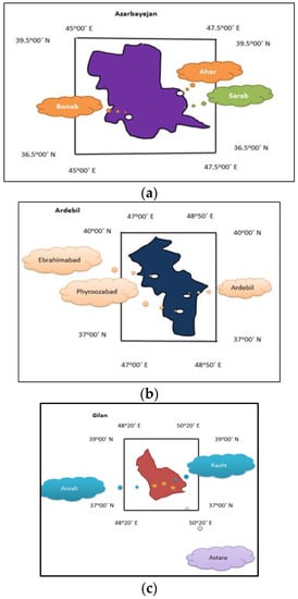
Figure 1.
Location of case study (a) East Azarbayjan, (b) Ardebil, and (c) Gilan.
A moderate climate is observed in this basin. The area of this province is 14,044 km2, and the average annual precipitation varied from 1200 to 1800 mm during the period from 2008 to 2018. The climatology-oriented Rasht Institute (longitude: 49°39′ and latitude: 37°12′), Anzali (longitude: 49°39′ and latitude: 38°20′) and Astara (longitude: 48°51′ and latitude: 38°21′) are used to record the different data. The AQI at the different stations is computed based on the following equation:
where I is the air quality index, C is the pollutant concentration, is the concentration extreme equal to or lower than C, is the concentration extreme equal to or greater than C, Ihigh is the index breakpoint related to , and Ilow is the index breakpoint related to . Table 1 shows the different classifications of AQI (Air Quality Index).

Table 1.
Classification of the AQI index.
Figure 2 shows the average AQI during different months in Ardebil, East Azarbayejan, and Gilan Provinces. Clearly, the greatest variation in East Azarbayejan can be observed in January as follows: The minimum AQI in January is 46, and the maximum value is 74. The lowest variation in East Azarbayejan is observed in May (minimum AQI = 60 and maximum AQI = 62). The highest AQI value is observed in March (AQI = 79.5) in East Azarbayejan, and the lowest AQI value in East Azarbayejan Province (EAZP) occurs in April. This index in EAZP shows that the first quartile and third quartile in most months exhibit an AQI > 50, and the conditions appear to differ only in April. The other values of the AQI index can be observed in the other provinces.
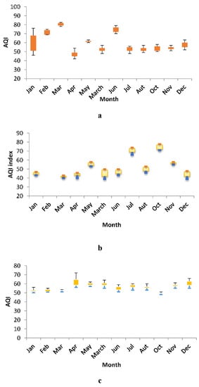
Figure 2.
AQI for (a) East Azarbayjan, (b) Ardebil, and (c) Gilan.
Table 2 shows the variation in the average temperature during the different months during the period of 2008–2018. July exhibits the greatest variation based on the high value of the variation coefficient in Azarbayejan (EAZP), and the maximum temperature in this province occurs during this month. The minimum temperature in Ardebil Province (AP) occurs in January, and the greatest variation in this province can be observed in May. The other details are listed in Table 2. Figure 3 shows the precipitation values in the different provinces. For example, the highest precipitation value in AP occurs in March, and the greatest variation in precipitation in AP is observed in this month. The lowest precipitation value in AP occurs in December. The other details of the other provinces are shown in Figure 3. Additionally, the number of sunny hours at different stations is shown. For example, the number of sunny hours (NSN) in June in Gilan Province (GP) is as follows: The most variation in the NSN occurs in June, and the lowest variation can be observed in July. The other details are shown in Figure 3.
Table 2.
Temperature variation for the different months (2008–2019).
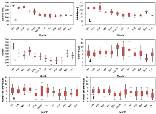
Figure 3.
(a) Monthly temperature for the 2008–2018 in EAZP, (b) monthly temperature for the 2008–2018 in AP, (c) monthly temperature for the 2008–2018 in GP, (d) monthly number of sunny hours for the 2008–2018 in EAZP, (e) monthly number of sunny hours for the 2008–2018 in AP, (f) monthly number of sunny hours for the 2008–2018 in GP.
The inverse distance weight (IDW) method was used to obtain the SR in the different zones. This method has an effective feature allowing the optimal value to be obtained based on a multi-objective optimization framework as follows:
where is the estimated precipitation at each point, Di is the difference between the predicted and observed data, and q is the power parameter.
Three objective functions are considered in the ANFISmulti-objective optimization algorithm [40]. The obg function is considered to select the best input parameters for the ANFIS, and the RMSE is used as an objective function to obtain the best value of the ANFIS parameters. The general standard deviation (GSD) is used to obtain the optimal power parameter for the IDW:
where is the training data number, RMSEtrain is the root mean square error of the training data, is the root mean square error of the test data, is the mean absolute error of the training data, is the mean absolute error of the test data, is the correlation coefficient of the training data, is the correlation coefficient of the test data, Ti represents the simulated data, is the average value of the simulated data at different points, and Oi represents the observed data. Lower RMSE, MAE, and GSD values are considered better. First, the ANFIS model is considered based on the initial estimates of the linear and nonlinear parameters, and different components (Ns: Number of sunny hours, Tmax(t−3): Maximum temperature with a three-month lag, Tmax(t−6): Maximum temperature with a 6-month lag, Tmin(t−3): Minimum temperature with a three-month lag, Tmin(t−6): Minimum temperature with a six-month lag, Rainfall(t−3): Precipitation value with a three-month lag, Rainfall(t−6): Precipitation value with a six-month lag, and the AQI indexes) are used as inputs. The ANFIS simulates the results. The IDW is used to simulate SR in the different zones, and then, the Multi-Objective Shark Algorithm (MOSA) is used based on the initial population used for the selection of inputs, the optimal determination of the adaptive neuro-fuzzy inference system (ANFIS) parameters, and the selection of the power parameters for the IDW. As shown in Figure 4, the different operators apply the candidate solutions, and then, these solutions are returned to the ANFIS subroutine for another simulation iteration. If the stopping criteria are satisfied, the process finishes with the optimal results. The modified technique for order preference by similarity by the ideal solution (M-TOPSIS) is used to select the best solution from the Pareto form based on the following equations:
where xj+ is the ideal solution (largest maximization criterion value or smallest minimization criterion value), xj− is the negative ideal solution (largest minimization criterion value or smallest maximization criterion value), is the distance from the ideal solution, is the distance from the least ideal solution, xij represents the results of alternative i considering criterion j, and is the similarity ratio, and this index of the solution is sorted by descending values to show the rank of each solution.
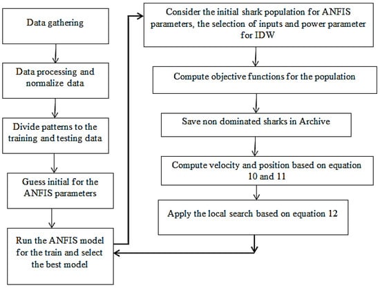
Figure 4.
MOSA and ANFIS structure.
Additionally, the following indexes are used to select the best multi-objective algorithm:
● Cover Surface (CS)
This index presents the relative score of the solutions in set B that are weakly dominated by set A as follows:
If the index value equals 1, all solutions in set B are weakly dominated by those in set A, and if the index value equals −1, any solution in set B is dominated by the solutions in set A. However, the index value can have values other than 1 and −1, which could indicate that the number of solutions in set A is covered by those in set B.
● General Distance (GD)
This index shows the closeness value of the computed Pareto solutions to the true Pareto solution. If Q is considered a set obtained by the MOSA, the GD is computed based on the following equation:
where P* is a reference solution (a set of all possible true Pareto solutions), is the distance of the solution obtained by the algorithm to the best solution, and is the m-objective value of the kth member of P*. A lower value of this index is more favorable for decision makers.
● Spread Index (SI)
The SI presents the diversity value of the obtained and archived solutions among the non-dominated solutions.
where di is the Euclidean distance between successive solutions among the obtained non-dominated solutions, is the average of all distances di, N is the number of solutions in the best non-dominated front, and is the computed distance of the extreme solution between the obtained Pareto of the moth objective and the true optimal Pareto.
● Spacing Metric (SM)
This index is computed by measuring the distances of successive solutions in a non-dominated front and shows an evaluation of the spread of vectors in the total set of non-dominated solutions.
where , and fik is the value of the ith objective function of the kth member.
5. Discussion and Results of the Algorithm Parameters
5.1. Results of the Sensitivity Analysis
Evolutionary algorithms are usually initialized using random parameters to allow accurate prediction values to be determined when these random parameters have been optimally selected. The Taguchi model is used to set the values of the random parameters. Its advantages include decreased time and cost in the selection of effective parameters with respect to the results. The selection of an orthogonal array is important for the Taguchi model. Table 3 shows the effective parameters of each algorithm. For example, the MOSA has four effective parameters with four levels, and the other details of the other algorithms are also shown. Then, the relative deviation index (RDI) is used based on the computed CS, GD, SI, and SM values.
Table 3.
Level and effective parameters for MOSA, NSGAII, and MOPSO ( Multi objective particle swarm algorithm.
In fact, this index shows the difference among the computed solutions with the best solution in each index. Notably, the best solution in some indexes, such as the CS, is considered based on the computed largest value of this index, and the best solution in other indexes, such as the GD, SI, and SM, is computed based on the lowest value of the indexes.
where is the computed solution of each index, and is the best computed solution of each index.
When the RDI is computed for the CS, GD, SI, and SM, the product of a Wight parameter (WP) and the computed RDI is obtained, and then, the products of the RDI and WP for the different indexes are summed. The WP of the SC, GD, SI, and SM is 0.25 because the four indexes have the same priority to decision makers, and the algorithm should satisfy all indexes. Then, Minitab software is used, and the L9, L12, and L9 arrays of the MOSA, NSGAII, and MOPSO, respectively, are considered for the model. The orthogonal array and results are shown in Table 4. The lowest CMRDI value shows that the algorithm parameters can obtain the solutions with a small difference between the best solutions. For example, the size population for the MOSA with level 2 has the lowest value among the levels, and thus, the population size for level 2 equals 30. The best values of the other parameters can be computed similarity. The best CMRDI value is shown in Table 4.
Table 4.
Computed results based on the computed average of the relative deviation index (CMRDI) for MOSA, MOPSOA, and NSGAII.
5.2. Results of the Different Multi-Objective Algorithms
The three Pareto fronts of the three algorithms are shown in Figure 5. The results and discussion were applied to Azarbayejan Province to avoid repetition. Additionally, when a large Pareto is obtained, many points act as solutions, and thus, the methods are compared using a decreased number of points for ease of presentation and to facilitate understanding (Table 5). A cluster method was used in the current article. First, the N cluster is considered, and the distance between each cluster is computed. The two clusters with the smallest distance are selected and combined to generate one cluster, and this process continues until the number of clusters reaches the lowest probable value. Linear programming is used to obtain each objective function value separately without considering the other two objective functions. B, C, and A are the best values of the first objective function (F(1) or GSD), the second objective function (F(2) or RMSE), and third objective function (F(3) or MAE), respectively. By comparing the nearest points of the different algorithm Pareto results to the mentioned points (A, B, and C), in contrast to the cases of the other algorithms, the nearest point in the MOPSO can obtain and match the optimal objective function separately. For the ease of comparison, the objective function values are converted to values between 0 and 1. A, B, and C have the best optimal values for the three objective functions, F(3), F(1), and F(2), respectively, based on the lowest values. Thus, the value of the objective function of the ideal points is considered the closest value to 1; consequently, the other points could be sorted and ranked. Additionally, the nearest points (NPs) to the reference points A, B, and C in the MOSA, MOPSO, and NSGAII are shown by NPMOSA, NPMOPSO, and NPNSGAII, respectively. Clearly, the NPMOSA has a good match with the best optimal objective function. For example, the best value of F(1) based on the B point is considered equal to 1, and this value of NPMOSA is 0.99; the other points are similar. In fact, when F(1) equals 1, the best objective function value of F(1) can be observed in point B, and then, F(2) and F(3) are computed for this point. Clearly, when an ideal point can satisfy one objective function, the value of the other objective functions at this point does not have the best value. In addition, the results of the other two provinces are shown in Figure 5. Figure 6 shows the RDI percentage of the different indexes in Azarbayejan, and the values in Ardebil and Gilan are not shown in this section to avoid repetition. The low RDI value shows better solutions and Pareto for the multi-objective algorithms. Notably, the variation in the values of the different indexes in the MOSA is smaller than that using the other two methods, and thus, the reliability of the generated data based on the ANFIS-MOSA is higher than that of the other algorithms. Additionally, the minimum, maximum, and median RDI in the box plots of the NFIS-SOMA have lower values than those based on the other two algorithms. Thus, these results show that the formed Pareto for the ANFIS-MOSA has good and diverse distribution in the space problem compared with that for the other two algorithms. Notably, the input data in each separate province during different months are associated with separate outputs per province.
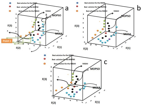
Figure 5.
Pareto front for (a) Azarbayjen province, (b) Ardebil, and (C) Gilan.
Table 5.
Comparison of the condition of the nearest point of each Pareto with the best values of each objective function for Azarbayejan.
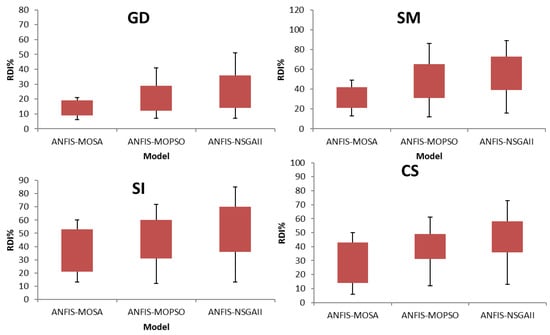
Figure 6.
Computation of RDI for different indexes for Azarbayejan province.
5.3. SR Results
The previous section showed that the ANFIS-MOSA has better performance than the other two models. There are initially 10 points representing the MOSA Pareto in Figure 5. The points are labelled by a number such that point 1 is shown by the number 1, and the other numbers corresponding to the other points are allocated such that the sixth point representing the MOSA and its Pareto is based on the MTOPSIS. This index is based on the objective function value and the difference in the objective function at each point between the most ideal and least ideal points. Then, the similarity ratio is computed for each point, and the points are sorted based on the computed rank. Figure 5 shows the best solution for EAZP, and the points are computed for other similar points such that each point shows a combination of the input, the value of the q power, and the optimal values for the ANFIS model. For example, the best point for the MOSA simulates SR with inputs (Ns: Number of sunny hours, Tmax(t−3): Maximum temperature with a three-month lag, Tmin(t−3): Minimum temperature with a three-month lag, rainfall(t−3): Precipitation value with a three-month lag, and AQI indexes), and the other points have different input combinations. Clearly, the best model or sixth point in the MOSA Pareto and EAZP does not use all inputs, and thus, this model can obtain the best results with the fewest number of inputs. Figure 7 compares the performance of 10 points in the ANFIS-MOSA, and the Taylor diagram is based on the standard deviation, correlation, and distance from the reference point. The numbers on the radius show the RMSE values. The performance of the sixth point in different provinces shows better simulation results because it is closer to the reference point and, thus, shows the best performance.
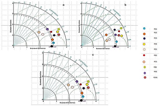
Figure 7.
The results for the Pareto solutions for (a) EAZP, (b) AP, and (c) GP.
Figure 8 shows the process variation of the RMSE, MAE, and NSE indexes for the 10 points in the different provinces, and the locations of the points are determined on the three-dimensional graph. Clearly, the sixth point has the lowest RMSE and MAE values and the highest NSE value. In fact, the 10 points show that 10 combination inputs were generated by the MOSA and that the sixth point has the best input combination, best value of the ANFIS parameter, and best value of the power q for the IDW. The locations of the points are shown in Figure 8. Stars show the points. Table 6 shows the performance of the ideal solution of ANFIS and MOSA with and without the AQI input parameter. The results show that the elimination of the AQI input parameter significantly increases the error index and decreases the NSE because the elimination of this parameter enables the simulation of SR. Although the dependency of the performance of models to AQI is variable for different studies, it is essential to consider the AQI as one of the model inputs for solar radiation. This is due to the fact that there is a strong interaction between the solar radiation value and air pollutant and visa-versa. For example, airborne particulate and gaseous pollutants decrease the amount of solar radiation reaching the Earth's surface. In contrast, ultraviolet (UV) radiation is necessary to initiate a series of reactions that cause high urban ozone values. Understanding the interaction between solar radiation and air pollution is especially important from the viewpoint of collecting and utilizing solar energy as an alternate energy source. Aerosols in the atmosphere can alter the solar radiation incident at the ground in two ways: By depleting the total energy and by changing the relative amounts of direct and diffuse radiation. At urban sites, high aerosol concentrations reduce the total incident energy and alter the direct: diffuse ratio. At rural locales, where anthropogenic aerosol burdens are smaller, the decrease in the direct solar beam will be largely compensated by an increase in the diffuse flux. Photo-chemical pollutants, which depend on UV radiation for their formation, also affect the amount of solar energy reaching the ground. Ozone and the particles formed from photochemically induced gas to particle reactions cause absorption and scattering of incident radiation. As a result, the air pollution is one of the most effective parameters that influences on the expected value of the solar radiation. However, it is relatively difficult to understand the real interrelationship between them mathematically. In addition, in most case studies, the data for air pollution is not available. Therefore, it is necessary while developing a model for forecasting solar radiation to consider the air pollution as one of the major inputs to the model. It can be obviously observed from Table 6 that the expected errors could be increased especially if the pollution value has a high level.
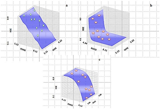
Figure 8.
The tree generated three dimensional figure based on all solutions in Pareto with the determination of 10 points of the Pareto solution in the ANFIS-MOSA model for (a) the test level in EAZP, (b) test level in AP, and (c) test level in GP.
Table 6.
Consideration of ANFIS and MOSA model with and without AQI for the best solution.
Figure 9 shows the zone map based on the IDW and AQI in EAZPs for different seasons. The Kappa coefficient is used as an index to show the degree of agreement between the observation zone map and the obtained map based on the ANFIS and IDW. The Kappa values of SR in the winter, autumn, summer, and spring are 0.85, 0.89, 0.91, and 0.92, respectively, highlighting the high accuracy of the zone map. The zone map of winter shows a lower intensity in most areas of the map, and that of summer shows a higher SR intensity.
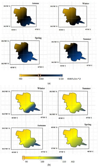
Figure 9.
(a) The AQI variation for different provinces based on obtaining zoning map, (b) the zoning map for the SR.
The analysis of the results shows that the AQI value in the winter season has a greater intensity than that in the other seasons. In fact, the higher concentration of pollutant particles in the winter season significantly increases the AQI value, and these particles decrease the SR intensity. Thus, if a decision maker eliminates the AQI, the zone map of the SR in winter is drawn as a sample, and the zone map shows higher SR in the different parts of the zone map in the winter. Thus, the elimination of the AQI significantly increases the SI, highlighting the importance of considering the AQI as an input. Another point is related to the uncertainty of the simulated results because the input data and the IDW method used for the zone map contain uncertainty; thus, the computation of the uncertainty of the model is very important, and therefore, generalized likelihood uncertainty estimation (GLUE) was used in this article. When the variation domain of the input parameters of the best solution in the ANFIS and MOSA is determined, sampling is applied to the parameter space. First, the space parameter is divided into the same interval, and then, sampling is considered for each interval [41]. Thus, when the gathered parameters are obtained and compared, a series of initial parameters is prepared to be inserted into the ANFIS model. The sampling of data is repeated 10,000 times, and then, the model based on the data group (generated sample) and the computation of the probability value based on the observed data and simulated data are considered such that the input parameters are generated based on 10,000 iterations.
The objective functions are computed for 10,000 iterations, and all SR simulated data are sorted after arranging the objective function values. Then, 2.5% of the data of the upper limit and 2.5% of the data of the lower limit are considered as outlying data. Thus, the bound of 95% of the certainty level is considered, and the d factor shows the thickness bound (Figure 10).
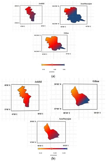
Figure 10.
The zoning maps for the provinces based on uncertainty of data based on (a) p factor and (b) d value.
The p values show the percentage of data in the 95% boundary, and a higher percentage corresponds to the better performance of each method. When the zone map based on the IDW is obtained, the value, p factor, and d factor of the data from each area of the zone map are computed to show the uncertainty value of the estimated results on the complete map. Clearly, the d factor is small, and the p factor exhibits a good percentage of the maps (Figure 10).
6. Conclusions
The current paper aimed to simulate SR based on the ANFIS-MOSA, and the IDW was used to obtain zone maps of three provinces. Pareto solutions were obtained using different algorithms and the ANFIS model. The different indexes showed that ANFIS-MOSA performs better than the other models, and the low value of the RDI index showed that the Pareto obtained using the MOSA and ANFIS matched well with the ideal solution. The MTOPSIS model was used to select the optimal solutions, and different indexes, such as the RMSE, MAE, and Taylor diagram, showed that the obtained ideal solution performance was the highest for the Pareto solution with a significant difference. Then, the effect of the AQI parameter on the results was analyzed. The results showed that the elimination of the AQI parameter decreased the accuracy of the zone map. Additionally, different models with and without the AQI parameter were considered, and the results showed that the error index without the AQI parameter was significantly higher. Finally, the uncertainty of the obtained data was considered to determine its effect on the results, and the high p factor value and low d factor value illustrated the adequate performance of the proposed model. The proposed model can not only simulate SR with an acceptable level of accuracy but also add a new direction to include multi-objective functions to evaluate the performance of the prediction model. For example, to improve the performance of the proposed model, another objective function could be considered to represent the risk performance, such as experiencing ± maximum errors. In this context, an objective function that represents the risk performance could be added to address the probability occurrence of the ±maximum errors at any time during the span of the prediction time.
In fact, the current research focused on studying the performance of the proposed model considering the time period dimension. However, there is an important dimension that could be considered for further analysis, which is the importance of a certain parameter at a specific location. In this context, it is essential to recommend this direction of research to be carried out in future research.
Author Contributions
Formal analysis, M.E., A.N.A. and H.A.A.; methodology, M.E. and A.E.-S.; writing—original draft, M.E. and C.M.F.
Funding
The authors would like to appreciate the financial support received from Bold 2025 grant coded RJO 10436494 by Innovation & Research Management Center (iRMC), Universiti Tenaga Nasional, Malaysia and from research grant coded UMRG RP025A-18SUS funded by the University of Malaya.
Acknowledgments
The authors appreciate so much the facilities support by the Civil Engineering Department, Faculty of Engineering, University of Malaya, Malaysia.
Conflicts of Interest
The authors declare no conflict of interest.
Abbreviations
| AQI | air quality index |
| a,b,c | premise parameters |
| C1 | cognitive coefficient |
| C2 | Acceleration coefficient |
| CS | Cover surface |
| d | Euclidean distance |
| GD | General distance |
| IDW | inverse distance weight |
| K | Number of iteration |
| M | the number of point |
| NO | number of training data |
| ND | Number of decision variable |
| OF | objective function |
| R1 | Random number |
| R2 | Random number |
| R*j | similarity ratio |
| SI | spread index |
| SR | solar radiation |
| Up | upper constraints |
| Ub | lower constraint |
| Wi | Wight value |
| Xit+1 | new position |
| Xgbest | global solution |
| Xpbest | the personal best solution |
| vij | velocity |
| Zi | new position after rotational movement |
| Momentum coefficient |
References
- Quej, V.H.; Almorox, J.; Arnaldo, J.A.; Saito, L. ANFIS, SVM and ANN soft-computing techniques to estimate daily global solar radiation in a warm sub-humid environment. J. Atmos. Sol.-Terr. Phys. 2017, 155, 62–70. [Google Scholar] [CrossRef]
- Ma, M.; Zhao, L.; Deng, S.; Zhang, Y.; Lin, S.; Shao, Y. Estimation of horizontal direct solar radiation considering air quality index in China. Energy Procedia 2019, 158, 424–430. [Google Scholar] [CrossRef]
- De León-Ruiz, J.; Carvajal-Mariscal, I.; De León-Ruiz, J.E.; Carvajal-Mariscal, I. Mathematical thermal modelling of a direct-expansion solar-assisted heat pump using multi-objective optimization based on the energy demand. Energies 2018, 11, 1773. [Google Scholar] [CrossRef]
- Ghazvinian, H.; Mousavi, S.F.; Karami, H.; Farzin, S.; Ehteram, M.; Hossain, M.S.; Fai, C.M.; Hashim, H.B.; Singh, V.P.; Ros, F.C.; et al. Integrated support vector regression and an improved particle swarm optimization-based model for solar radiation prediction. PLoS ONE 2019, 14, e0217634. [Google Scholar] [CrossRef]
- Atuahene, S.; Bao, Y.; Ziggah, Y.; Gyan, P.; Li, F.; Atuahene, S.; Bao, Y.; Ziggah, Y.Y.; Gyan, P.S.; Li, F. Short-Term Electric Power Forecasting Using Dual-Stage Hierarchical Wavelet-Particle swarm optimization-adaptive neuro-fuzzy inference system PSO-ANFIS approach based on climate change. Energies 2018, 11, 2822. [Google Scholar] [CrossRef]
- Lotfinejad, M.; Hafezi, R.; Khanali, M.; Hosseini, S.; Mehrpooya, M.; Shamshirband, S.; Lotfinejad, M.M.; Hafezi, R.; Khanali, M.; Hosseini, S.S.; et al. Comparative assessment of predicting daily solar radiation using bat neural network (BNN), generalized regression neural network (GRNN), and neuro-fuzzy (NF) system: A Case Study. Energies 2018, 11, 1188. [Google Scholar] [CrossRef]
- Sharifi, S.S.; Rezaverdinejad, V.; Nourani, V. Estimation of daily global solar radiation using wavelet regression, ANN, GEP and empirical models: A comparative study of selected temperature-based approaches. J. Atmos. Sol.-Terr. Phys. 2016, 149, 131–145. [Google Scholar] [CrossRef]
- Alsina, E.F.; Bortolini, M.; Gamberi, M.; Regattieri, A. Artificial neural network optimisation for monthly average daily global solar radiation prediction. Energy Convers. Manag. 2016, 120, 320–329. [Google Scholar] [CrossRef]
- Yaseen, Z.; Ehteram, M.; Hossain, M.; Fai, C.; Binti Koting, S.; Mohd, N.; Binti Jaafar, W.; Afan, H.; Hin, L.; Zaini, N.; et al. A novel hybrid evolutionary data-intelligence algorithm for irrigation and power production management: Application to multi-purpose reservoir systems. Sustainability 2019, 11, 1953. [Google Scholar] [CrossRef]
- Meenal, R.; Selvakumar, A.I. Assessment of SVM, empirical and ANN based solar radiation prediction models with most influencing input parameters. Renew. Energy 2018, 121, 324–343. [Google Scholar] [CrossRef]
- Marzo, A.; Trigo-Gonzalez, M.; Alonso-Montesinos, J.; Martínez-Durbán, M.; López, G.; Ferrada, P.; Fuentealba, E.; Cortés, M.; Batlles, F.J. Daily global solar radiation estimation in desert areas using daily extreme temperatures and extraterrestrial radiation. Renew. Energy 2017, 113, 303–311. [Google Scholar] [CrossRef]
- Renno, C.; Petito, F.; Gatto, A. ANN model for predicting the direct normal irradiance and the global radiation for a solar application to a residential building. J. Clean. Prod. 2016, 135, 1298–1316. [Google Scholar] [CrossRef]
- Shamshirband, S.; Mohammadi, K.; Tong, C.W.; Zamani, M.; Motamedi, S.; Ch, S. A hybrid SVM-FFA method for prediction of monthly mean global solar radiation. Theor. Appl. Climatol. 2015, 125, 53–65. [Google Scholar] [CrossRef]
- Samadianfard, S.; Majnooni-Heris, A.; Qasem, S.N.; Kisi, O.; Shamshirband, S.; Chau, K. Daily global solar radiation modeling using data-driven techniques and empirical equations in a semi-arid climate. Eng. Appl. Comput. Fluid Mech. 2019, 13, 142–157. [Google Scholar] [CrossRef]
- Mehdizadeh, S.; Behmanesh, J.; Khalili, K. Comparison of artificial intelligence methods and empirical equations to estimate daily solar radiation. J. Atmos. Sol.-Terr. Phys. 2016, 146, 215–227. [Google Scholar] [CrossRef]
- Koca, A.; Oztop, H.F.; Varol, Y.; Koca, G.O. Estimation of solar radiation using artificial neural networks with different input parameters for Mediterranean region of Anatolia in Turkey. Expert Syst. Appl. 2011, 38, 8756–8762. [Google Scholar] [CrossRef]
- Ozgoren, M.; Bilgili, M.; Sahin, B. Estimation of global solar radiation using ANN over Turkey. Expert Syst. Appl. 2012, 39, 5043–5051. [Google Scholar] [CrossRef]
- Voyant, C.; Muselli, M.; Paoli, C.; Nivet, M.-L. Numerical weather prediction (NWP) and hybrid ARMA/ANN model to predict global radiation. Energy 2012, 39, 341–355. [Google Scholar] [CrossRef]
- Furlan, C.; de Oliveira, A.P.; Soares, J.; Codato, G.; Escobedo, J.F. The role of clouds in improving the regression model for hourly values of diffuse solar radiation. Appl. Energy 2012, 92, 240–254. [Google Scholar] [CrossRef]
- Chen, J.-L.; Li, G.-S.; Wu, S.-J. Assessing the potential of support vector machine for estimating daily solar radiation using sunshine duration. Energy Convers. Manag. 2013, 75, 311–318. [Google Scholar] [CrossRef]
- Vakili, M.; Sabbagh-Yazdi, S.-R.; Kalhor, K.; Khosrojerdi, S. Using artificial neural networks for prediction of global solar radiation in Tehran considering particulate matter air pollution. Energy Procedia 2015, 74, 1205–1212. [Google Scholar] [CrossRef]
- Quesada-Ruiz, S.; Linares-Rodríguez, A.; Ruiz-Arias, J.A.; Pozo-Vázquez, D.; Tovar-Pescador, J. An advanced ANN-based method to estimate hourly solar radiation from multi-spectral MSG imagery. Sol. Energy 2015, 115, 494–504. [Google Scholar] [CrossRef]
- Çelik, Ö.; Teke, A.; Yıldırım, H.B. The optimized artificial neural network model with Levenberg–Marquardt algorithm for global solar radiation estimation in eastern mediterranean region of Turkey. J. Clean. Prod. 2016, 116, 1–12. [Google Scholar] [CrossRef]
- Deo, R.C.; Şahin, M. Forecasting long-term global solar radiation with an ANN algorithm coupled with satellite-derived (MODIS) land surface temperature (LST) for regional locations in Queensland. Renew. Sustain. Energy Rev. 2017, 72, 828–848. [Google Scholar] [CrossRef]
- Yao, W.; Zhang, C.; Wang, X.; Sheng, J.; Zhu, Y.; Zhang, S. The research of new daily diffuse solar radiation models modified by air quality index (AQI) in the region with heavy fog and haze. Energy Convers. Manag. 2017, 139, 140–150. [Google Scholar] [CrossRef]
- Loghmari, I.; Timoumi, Y.; Messadi, A. Performance comparison of two global solar radiation models for spatial interpolation purposes. Renew. Sustain. Energy Rev. 2018, 82, 837–844. [Google Scholar] [CrossRef]
- Fan, J.; Wu, L.; Zhang, F.; Cai, H.; Wang, X.; Lu, X.; Xiang, Y. Evaluating the effect of air pollution on global and diffuse solar radiation prediction using support vector machine modeling based on sunshine duration and air temperature. Renew. Sustain. Energy Rev. 2018, 94, 732–747. [Google Scholar] [CrossRef]
- Khan, I.; Zhu, H.; Yao, J.; Khan, D.; Iqbal, T. Hybrid power forecasting model for photovoltaic plants based on neural network with air quality index. Int. J. Photoenergy 2017, 2017. [Google Scholar] [CrossRef]
- Wang, H.; Sun, F.; Wang, T.; Liu, W. Estimation of daily and monthly diffuse radiation from measurements of global solar radiation a case study across China. Renew. Energy 2018, 126, 226–241. [Google Scholar] [CrossRef]
- Sun, H.; Gui, D.; Yan, B.; Liu, Y.; Liao, W.; Zhu, Y.; Lu, C.; Zhao, N. Assessing the potential of random forest method for estimating solar radiation using air pollution index. Energy Convers. Manag. 2016, 119, 121–129. [Google Scholar] [CrossRef]
- Vakili, M.; Sabbagh-Yazdi, S.R.; Khosrojerdi, S.; Kalhor, K. Evaluating the effect of particulate matter pollution on estimation of daily global solar radiation using artificial neural network modeling based on meteorological data. J. Clean. Prod. 2017, 141, 1275–1285. [Google Scholar] [CrossRef]
- Mohammad-Azari, S.; Bozorg-Haddad, O.; Chu, X. Shark smell optimization (SSO) algorithm. Adv. Optim. Nat.-Inspir. Algorithms 2017, 93–103. [Google Scholar]
- Ehteram, M.; Karami, H.; Mousavi, S.-F.; El-Shafie, A.; Amini, Z. Optimizing dam and reservoirs operation based model utilizing shark algorithm approach. Knowl.-Based Syst. 2017, 122, 26–38. [Google Scholar] [CrossRef]
- Abedinia, O.; Amjady, N.; Ghasemi, A. A new metaheuristic algorithm based on shark smell optimization. Complexity 2014, 21, 97–116. [Google Scholar] [CrossRef]
- Santiago, A.; Dorronsoro, B.; Nebro, A.J.; Durillo, J.J.; Castillo, O.; Fraire, H.J. A novel multi-objective evolutionary algorithm with fuzzy logic based adaptive selection of operators: FAME. Inf. Sci. 2019, 471, 233–251. [Google Scholar] [CrossRef]
- Deb, K.; Pratap, A.; Agarwal, S.; Meyarivan, T. A fast and elitist multiobjective genetic algorithm: NSGA-II. IEEE Trans. Evol. Comput. 2002, 6, 182–197. [Google Scholar] [CrossRef]
- Mofid, H.; Jazayeri-Rad, H.; Shahbazian, M.; Fetanat, A. Enhancing the performance of a parallel nitrogen expansion liquefaction process (NELP) using the multi-objective particle swarm optimization (MOPSO) algorithm. Energy 2019, 172, 286–303. [Google Scholar] [CrossRef]
- Antonakis, A.; Nikolaidis, T.; Pilidis, P.; Antonakis, A.; Nikolaidis, T.; Pilidis, P. Multi-objective climb path optimization for aircraft/engine integration using particle swarm optimization. Appl. Sci. 2017, 7, 469. [Google Scholar] [CrossRef]
- Wang, Y.; Hua, Z.; Wang, L.; Wang, Y.; Hua, Z.; Wang, L. Parameter estimation of water quality models using an improved multi-objective particle swarm optimization. Water 2018, 10, 32. [Google Scholar] [CrossRef]
- Ehteram, M.; Afan, H.A.; Dianatikhah, M.; Ahmed, A.N.; Fai, C.M.; Hossain, M.S.; Allawi, M.F.; Elshafie, A.; Ehteram, M.; Afan, H.A.; et al. Assessing the predictability of an improved ANFIS model for monthly streamflow using lagged climate indices as predictors. Water 2019, 11, 1130. [Google Scholar] [CrossRef]
- Karimi, S.; Amiri, B.J.; Malekian, A. Similarity metrics-based uncertainty analysis of river water quality models. Water Resour. Manag. 2019, 33, 1927–1945. [Google Scholar] [CrossRef]
© 2019 by the authors. Licensee MDPI, Basel, Switzerland. This article is an open access article distributed under the terms and conditions of the Creative Commons Attribution (CC BY) license (http://creativecommons.org/licenses/by/4.0/).