Abstract
This survey paper describes a literature review of deep learning (DL) methods for cyber security applications. A short tutorial-style description of each DL method is provided, including deep autoencoders, restricted Boltzmann machines, recurrent neural networks, generative adversarial networks, and several others. Then we discuss how each of the DL methods is used for security applications. We cover a broad array of attack types including malware, spam, insider threats, network intrusions, false data injection, and malicious domain names used by botnets.
1. Introduction
Cyber security is the collection of policies, techniques, technologies, and processes that work together to protect the confidentiality, integrity, and availability of computing resources, networks, software programs, and data from attack. Cyber defense mechanisms exist at the application, network, host, and data level. There is a plethora of tools—such as firewalls, antivirus software, intrusion detection systems (IDSs), and intrusion protection systems (IPSs)—that work in silos to prevent attacks and detect security breaches. However, many adversaries are still at an advantage because they only need to find one vulnerability in the systems needing protection. As the number of internet-connected systems increases, the attack surface also increases, leading to greater risk of attack. Furthermore, attackers are becoming more sophisticated, developing zero-day exploits and malware that evade security measures, enabling them to persist for long periods without notice. Zero-day exploits are attacks that have not been encountered previously but are often variations on a known attack. To exacerbate the problem, attack mechanisms are being commoditized, allowing for rapid distribution without needing an understanding for developing exploits. In addition to defending against external threats, defenders also must guard against insider threats from individuals or entities within an organization that misuse their authorized access.
Throughout an attack’s lifecycle, there are indicators of compromise; there may even be significant signs of an impending attack. The challenge is in finding these indicators, which may be distributed across the environment. There are massive quantities of data from applications, servers, smart devices, and other cyber-enabled resources generated by machine-to-machine and human-to-machine interactions. Cyber defense systems are generating voluminous data, such as the Security Information Event Management (SIEM) system, which often overwhelms the security analyst with event alerts. The use of data science in cyber security can help to correlate events, identify patterns, and detect anomalous behavior to improve the security posture of any defense program. We are starting to see an emergence of cyber defense systems leveraging data analytics. For instance, network intrusion detection systems (NIDSs) that inspect packet transmissions are evolving from signature-based systems that detect well-known attacks to anomaly-based systems that detect deviations from a “normal” behavior profile.
This paper is intended for readers who wish to begin research in the field of deep learning (DL) for cyber security. Although DL is a subset of machine learning, it is a newer and more complex way of learning than the norm. As such, great emphasis is placed on a thorough description of the DL methods, and references to seminal works for each DL method are provided. Also, examples are included to illustrate how the techniques have been used in cyber security. Special emphasis was placed on highly-cited papers because these describe popular techniques. However, it is recognized that this emphasis might overlook significant new and emerging techniques, so some less-cited papers were chosen as well. Overall, papers were selected so that each of the DL categories listed subsequently had at least one, but preferably a few, representative papers.
Related surveys, such as those in [1,2,3,4,5,6] have described machine learning applications to cyber problems but did not include DL methods. Other authors describe DL methods for cyber security, but those methods have a narrow set of cyber security applications. The paper by Xin et al. [7] focuses exclusively on cyber-attacks related to intrusion detection and targets shortcomings in datasets and areas of research for future model development. In [8], the authors summarize work covering attacks related exclusively to intrusion detection, malware analysis, and spam detection, and do not cover malicious domain names commonly used by botnets. In [9], the authors reviewed and summarized work focusing on defending cyber-physical systems. Additionally, [10] reviews machine learning and DL methods for securing Internet of Things (IoT) technology. This paper is unique because it covers a wide array of cyber-attack types, and the approaches to detect them span a spectrum of DL techniques including convolutional neural networks (CNNs), recurrent neural networks (RNNs), and generative adversarial networks (GANs).
The remainder of this paper is organized as follows: Section 2 focuses on the foundations of DL compared to shallow learning. Section 3 overviews different DL methods used in cyber security. Section 4 describes several classification metrics employed in the papers. Section 5 discusses cybersecurity datasets for DL, and Section 6 discusses cyber applications of deep-learning methods. Section 7 provides observations and recommendations, and Section 8 concludes the paper with a brief summary of the paper’s key points and other closing remarks.
2. Shallow Learning vs. Deep Learning
Artificial neural networks (ANNs) are machine learning algorithms inspired by the central nervous system. They were first conceived in 1943 when McCulloch and Pitts [11] published a study presenting the mathematical model based on biological neuron. This was later implemented by Hebb [12] and Rosenblatt [13] in their development of unsupervised through self-organized learning and supervised learning through the creation of perceptrons, respectively. They are composed of a few layers of neurons connected by adaptive weights (Figure 1), and the adjacent network layers are usually fully connected. The universal approximation theorem for ANNs states that every continuous function that maps intervals of real numbers to some output interval of real numbers can be approximated arbitrarily closely by a multi-layer perceptron (type of ANN) with just one hidden layer. This means that an ANN with one hidden layer is capable of producing any non-linear continuous function, and as such much of the early research on ANNs concentrated on networks with just one hidden layer, trained using back-propagation [14]. Networks with just one hidden layer belong to the category of shallow learning. There are unsupervised and supervised shallow network architectures. Supervised learning uses labels (ground truth) to learn a task; unsupervised learning is performing a machine learning task without labels. In shallow learning, feature extraction is performed separately, not as a part of the network.
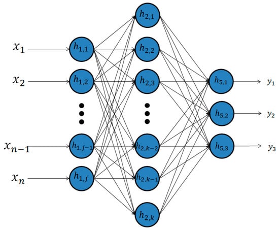
Figure 1.
Shallow neural network.
DL is a much newer endeavor, with the first computer implementation achieved in 2006 [9]. There are many definitions of DL and deep neural networks (DNNs). A simple definition states that DL is a set of machine learning algorithms that attempt to learn in multiple levels, corresponding to different levels of abstraction (Figure 2). The levels correspond to distinct levels of concepts, where higher-level concepts are defined from lower-level ones, and the same lower-level concepts can help to define many higher-level concepts [15]. Feature extraction is performed by the first few layers of the deep network. There are unsupervised, supervised, and hybrid DL architectures. Because shallow neural networks have only one hidden layer, they lack the ability to perform advanced feature extraction and are unable to learn the higher-level concepts that deep neural networks are capable of learning. This also holds true for other machine learning algorithms, as well. However, DL methods require greater computational power, sometimes multiple graphical processing units (GPUs), to train DL models in a reasonable time. Two advancements have made it possible for an average person to easily develop DL models. The first is the increased availability of GPUs, which allow for significantly faster computation. The second is the fact that the layers with a DL model can be trained independently of each other [16]. This means that a large model with millions of parameters can be optimized in small, manageable chunks, requiring significantly fewer resources.
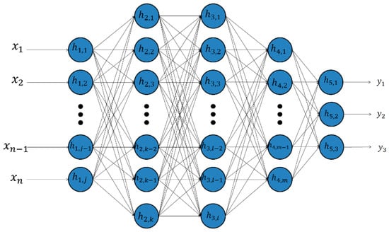
Figure 2.
Deep neural network.
The main difference between shallow and deep networks lies in the number of hidden layers; DL architectures have multiple hidden layers whereas shallow neural networks have at most one hidden layer.
In an ANN or DNN, a nonlinear function is applied to a weighted sum of the units in the previous layer. There are a number of different nonlinear functions that can be used; however, the most common are the sigmoid function, the softmax function, the hyperbolic tangent function, and the rectified linear unit (ReLU), which is simply f(z) = max(z.0). Although ReLUs were originally proposed in the 1970s [17], they gained widespread use only in 2009 [18].
3. Deep Learning Methods Used in Cyber Security
This section describes the different DL methods used in cyber security. References to important methodology papers are provided for each technique.
3.1. Deep Belief Networks
A seminal paper by Hinton [9] introduced Deep Belief Networks (DBNs). They are a class of DNNs composed of multiple layers of hidden units with connections between the layers but not between units within each layer. DBNs are trained in an unsupervised manner. Typically, they are trained by adjusting weights in each hidden layer individually to reconstruct the inputs.
3.1.1. Deep Autoencoders
Autoencoders are a class of unsupervised neural networks in which the network takes as input a vector and tries to match the output to that same vector. By taking the input, changing the dimensionality, and reconstructing the input, one can create a higher or lower dimensionality representation of the data. These types of neural networks are incredibly versatile because they learn compressed data encoding in an unsupervised manner. Additionally, they can be trained one layer at a time, reducing the computational resources required to build an effective model. When the hidden layers have a smaller dimensionality than the input and output layers (Figure 3), the network is used for encoding the data (i.e., feature compression). An autoencoder can be designed to remove noise and be more robust by training an autoencoder to reconstruct the input from a noisy version of the input (Figure 4), called a denoising autoencoder [19]. This technique has been shown to have more generalizability and robustness than typical autoencoders.
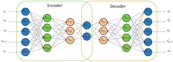
Figure 3.
Deep autoencoder.
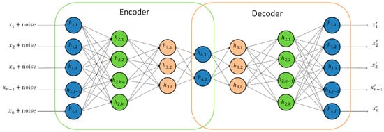
Figure 4.
Denoising autoencoder.
Using multiple layers of autoencoders, trained in series, to gradually compress the information more and more is called stacked autoencoders [20] (Figure 5). Figure 5a is the completed stacked autoencoder with a classification layer. It is formed by creating an autoencoder Figure 5b. Then, the autoencoder Figure 5c is built using the outputs of Figure 5b as inputs. Once trained, these are combined together and a classification layer is added. Similar to regular autoencoders, denoising autoencoders can be stacked as well [19].
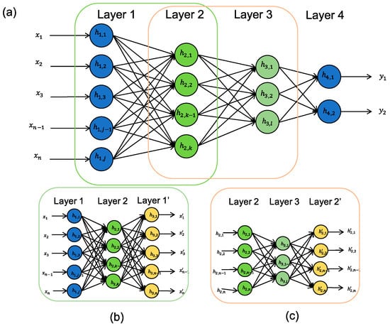
Figure 5.
Stacked autoencoder with a classification layer. (a) Stacked autoenoder; (b) autoencoder for layer 2; (c) autoencoder for layer 3.
A sparse autoencoder is a type of encoder wherein there are more hidden nodes than there are in the input and output layers, however, only a portion of the hidden units are activated at a given time [20,21]. This is accounted for by penalizing activating additional nodes.
3.1.2. Restricted Boltzmann Machines
Restricted Boltzmann machines (RBMs) are two-layer, bipartite, undirected graphical models (data can flow in both directions, rather than just one) that form the building blocks of DBNs [14]. Similar to autoencoders, RBMs are unsupervised and can be trained one layer at a time. The first layer is the input layer; the second layer is the hidden layer (Figure 6). There are no intra-layer connections (i.e., between nodes in the same layer); however, every node in the input layer is connected to every node in the hidden layer (i.e., full connectivity).

Figure 6.
Restricted Boltzmann machine.
Typically, the units in the input and hidden layers are restricted to binary units. The network is trained to minimize the “energy”, which is a function that measures the model’s compatibility, borrowing much of the mathematics from statistical mechanics. The aim in training the model is to find the functions, and therefore, the hidden state, that minimizes the energy of the system. Furthermore, RBMs are probabilistic, i.e., they assign probabilities instead of concrete values. However, the output can be used as features for another model. The model is trained by taking binary input data and feeding it forward through the model. Then, it is fed backwards through the model to reconstruct the input data. The energy of the system is then calculated and used to update the weights. This process is continued until the model converges.
Similarly, to autoencoders, RBMs can be stacked to form multiple layers to create a deeper neural network. These are referred to as stacked RBMs.
3.1.3. DBNs or RBMs or Deep Autoencoders Coupled with Classification Layers
Both RBMs and autoencoders can be combined with a classification layer (Figure 5) to perform a classification using a fully connected layer or layers. The layers trained by applying unsupervised learning are used as feature extractors, and they constitute inputs into the fully connected layers that are trained using back propagation. Unlike the RBM or autoencoder layers, these layers require labels to train [22]. These types of networks have shown success in a number of applications, including acoustic modeling [23], speech recognition [24], and image recognition [25].
3.2. Recurrent Neural Networks
A recurrent neural network (RNN), as shown on Figure 7, extends the capabilities of a traditional neural network, which can only take fixed-length data inputs, to handle input sequences of variable lengths. The RNN processes inputs one element at a time, using the output of the hidden units as additional input for the next element. Therefore, the RNNs can address speech and language problems as well as time series problems.
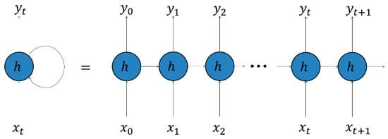
Figure 7.
Recurrent neural network.
Typically, RNNs are more difficult to train because the gradients can easily vanish or explode [26]. However, advancements in training and architecture have produced a variety of RNNs that are easier to train [27,28,29,30]. As a result, RNNs have shown success in next-word-in-a-sentence prediction, speech recognition, image captioning, language translation, and other time-series prediction tasks [31,32,33,34].
The hidden units of an RNN are capable of maintaining a “state vector” that contains a memory of the past events in the sequence. The length of this “memory” can be adjusted based on the type of RNN node that is used. The longer the memory, the longer term the dependencies the RNN is capable of learning.
The long short-term memory (LSTM) units [27] have been introduced to enable RNNs to manage problems that require long-term memories. LSTM units contain a structure called a memory cell that accumulates information, which it connects to itself in the next time step. The values of the memory cell are augmented by new input and a forget gate that weights newer and older information higher or lower depending on what is needed.
Another RNN unit that was designed for long memory is the gated recurrent unit (GRU) [32]. GRUs are similar to LSTM units but are designed to have fewer parameters, making them easier to train.
3.3. Convolutional Neural Networks
A convolutional neural network (CNN) [35,36] is a neural network meant to process input stored in arrays. An example input is a color or grayscale image, which is a two-dimensional (2D) array of pixels. CNNs are often used for processing 2D arrays of images or spectrograms of audio. They are also used frequently for three-dimensional (3D) arrays (videos and volumetric images). Their use to one-dimensional (1D) arrays (signals) is less frequent but increasing. Regardless of the dimensionality, CNNs are used where there is spatial or temporal ordering.
The architecture of a CNN (Figure 8) consists of three distinct types of layers: convolution layers, pooling layers, and the classification layer. The convolution layers are the core of the CNN. The weights define a convolution kernel applied to the original input, a small window at a time, called the receptive field. The result of applying these filters across the entirety of the input is then passed through a non-linearity, typically an ReLU, and is called a feature map. These convolution kernels, named after the mathematical convolution operation, allow close physical or temporal relationships within the data to be accounted for, and help reduce memory by applying the same kernel across the entirety of the image.
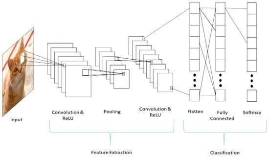
Figure 8.
Convolutional neural network.
Pooling layers are used to perform non-linear down sampling by applying a specific function, such as the maximum, over non-overlapping subsets of the feature map. Besides reducing the size of the feature maps, and therefore, the memory required, pooling layers also reduce the number of parameters, and therefore, overfitting. These layers are generally inserted periodically in between convolution layers and then fed into a fully connected, traditional DNN.
Additionally, CNNs can use regularization techniques that help reduce overfitting. One of the most successful techniques is called “dropout” [37]. When training a model using dropout, during each training iteration, a specified percentage of nodes in a given layer and their incoming and outgoing connections, are randomly removed. Including dropout typically improves the accuracy and generalizability of a model because it increases the likelihood a node will be useful.
Uses of CNNs are significantly varied. The greatest success has been achieved with computer vision tasks such as scene and object detection and object identification [38]. Applications range from biology [39] to facial recognition [40]. The best showcase of CNN success took place in 2012 at the ImageNet competition, where a CNN surpassed the performance of other methods, and then human accuracy in 2015 through the use of GPUs, ReLUs, dropout, and the generation of additional images [41]. In addition, CNNs have been used successfully in language models for phoneme detection [42], letter recognition [36], speech recognition [43], and language model building [44,45].
3.4. Generative Adversarial Networks
Generative adversarial networks (GANs), which are shown in Figure 9, are a type of neural network architecture used in unsupervised machine learning, in which two neural networks compete against each other in a zero-sum game to outsmart each other. Developed by Goodfellow et al. [46], one network acts as a generator and another network acts as a discriminator. The generator takes in input data and generates output data with the same characteristics as real data. The discriminator takes in real data and data from the generator and tries to distinguish whether the input is real or fake. When training has finished, the generator is capable of generating new data that is not distinguishable from real data.
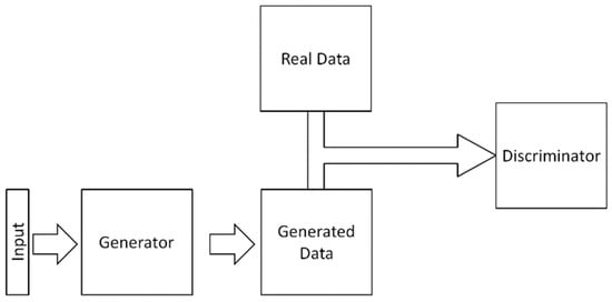
Figure 9.
Generative adversarial network.
Since first developed, GANs have shown wide applicability, especially to images. Examples include image enhancement [47], caption generation [48], and optical flow estimation [49]. Facebook even has an open-source, pre-trained GAN for image generation called deep convolution generative adversarial network (DCGAN) [50].
3.5. Recursive Neural Networks
Recursive neural networks are neural networks (Figure 10) that apply a set of weights recursively to a series of inputs. In these networks, the output of a node is used as input for the next step [51,52]. Initially, the first two inputs are fed into the model together. Afterward, the output from that is used as an input along with the next step. This type of model has been used for various natural language processing tasks [53,54,55,56] and image segmentation.
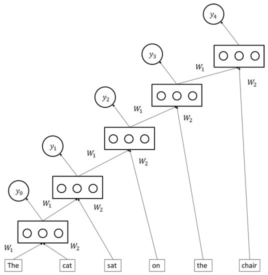
Figure 10.
Recursive neural network.
4. Metrics
This section describes several classification metrics used by the authors of the papers cited in the next sections. There are a number of different metrics for a model performing a binary classification task. These metrics include accuracy, precision, recall, false positive rate, F1 Score, and area under the curve (AUC) and many of the metrics have more than one name. All of these evaluation metrics are derived from the four values found in the confusion matrix (Table 1), which is based on the calculated predicted class versus the ground truth.

Table 1.
Confusion matrix.
Accuracy (acc) or Proportion Correct: the ratio of correctly classified examples to all items. The usefulness of accuracy is lower when the classes are unbalanced (i.e., there are a significantly larger number of examples from one class than from another). However, it does provide useful insight when the classes are balanced.
Positive Predictive Value (PPV) or Precision (p): The ratio of items correctly classified as class X to all items that were classified as class X.
Sensitivity or True Positive Rate (TPR) or Probability of Detection or Recall (r): The ratio of items correctly classified as X to all items that were actually class X.
Negative Predictive Value (NPV): The ratio of items correctly classified as not X to all items classified as not X.
Specificity or True Negative Rate (TNR): The ratio of items correctly classified as not X to all items that are not class X.
False Alarm Rate (FAR) or False Positive Rate (FPR) or Fall-Out: The ratio of items incorrectly classified as class X to all the items that are not class X.
F1 Score (): The F1 Score is the harmonic mean of the precision () and the true positive rate ().
This is a specific version of the F-β function, in which precision and true positive rate are given equal importance.
Area under the curve (AUC): The sum of the area under a receiver operating characteristic (ROC) curve, which is a plot of the false positive rate versus the true positive rate, created by varying the classification thresholds.
For multi-class problems, accuracy can be easily calculated; however, metrics such as precision, recall, FPR, F1 Score, and AUC cannot be calculated in a straightforward fashion (e.g., TP, TN do not exist for three-class problems). Precision, recall, etc. can be determined for a 3+ class problem by collapsing the problem into a two-class problem (i.e., all versus one), where the metrics are calculated for each class. Usually, only accuracy is used for multiclass problems.
It is important to remember that because each of the papers described later uses a different dataset (or sometimes a different subset of a given dataset), it is not possible to compare the models developed based on the accuracy (or any other metrics) they obtained. Such a comparison would be valid only if the authors of both publications used exactly the same training dataset and the same testing dataset.
5. Cybersecurity Datasets for Deep Learning
One of the most widely used datasets for intrusion detection is the Knowledge Discovery and Dissemination (KDD) 1999 dataset [57]. This dataset was created for the KDD Cup challenge in 1999 and is composed of more than 4 million network traffic records. However, the dataset does not include raw network traffic data. Instead, the raw pcap data has been preprocessed into 41 features based on basic type, content type, and traffic type features. The dataset contains 22 different kinds of attacks that fall into four families: denial of service (DoS), unauthorized access from a remote machine (R2L), unauthorized access to local super-user privileges (U2R), and probing. An analysis by [58], however, found there were a number of problems with the dataset. One major source of this was the synthetic nature of the network and attack data, dropped data due to overflow, and vague attack definitions. Furthermore, there were a large number of redundant records that biased the dataset. Because of these flaws, [58] proposed a new dataset called NSL-KDD, which is another frequently used dataset for network intrusion detection.
There are a few datasets that contain raw packet data; however, the most commonly used is the CTU-13 dataset [59]. This dataset contains raw pcap files for malicious, normal, and background data. The benefit of raw pcap files, compared to the KDD 1999 and NSL-KDD datasets, is the opportunity for individuals to perform their own preprocessing, enabling a wider range of algorithms to be used. Additionally, the CTU-13 dataset is not a simulated dataset. The botnet attacks are real, the unknown traffic is from a large network, and there is ground truth. It is a combination of 13 different scenarios with different numbers of computers and seven different botnet families, making it a diverse dataset.
There are three significant sources of data for domain generation algorithm (DGA) detection. Although there are previous ML papers that describe a variety of feature extraction techniques, the DL algorithms rely almost entirely on domain names. This is reflected in that the three primary sources of data for DGA detection are just domain names. The Alexa Top Sites [60] dataset is generally used as a source of benign domain names, as one can get as many as 1 million domain names. The malicious domain names are obtained from OSINT [61] and DGArchive [62]. The OSINT DGA feed from Bambenek Consulting was commonly used because it contains DGA domains from 50 different DGAs and includes more than 800 thousand malicious domain names. Alternatively, DGArchive provides access to more than 30 reverse-engineered DGAs, which can be used to generate malicious domain names on an internal network.
Malware datasets are far more common. The most common source of normal data in malware experiments are the top apps in the Google Play Store [63]. While these apps are not guaranteed to be malware free, they are the most likely to be malware free because of the combination of Google’s vetting and the ubiquity of the apps. In addition, they are sometimes vetted using the VirusTotal service [64]. There are a number of datasets that contain malware, including Contagio [65], Comodo [66], the Genome Project [67], Virus Share [68], VirusTotal [64], DREBIN [69], and Microsoft [70]. There is some overlap in the datasets that contain malicious data and the Google Play Store data, as that is where they obtained normal data.
Typically, malware datasets are saved as raw program files. This allows for an incredible amount of flexibility in terms of feature extraction and processing. The Genome Project dataset consists of 2123 applications, of which 1260 are malicious spanning 49 different malware families. This is similar to the Virus Share and VirusTotal datasets, which are a continuously updating repository of malware files, providing an ever-evolving list of new types of malware. The Comodo dataset is another large dataset containing 22,500 malicious and 22,500 benign raw files. The Contagio dataset is significantly smaller than the others, containing 250 malicious files. The DREBIN dataset is a highly imbalanced dataset containing 120,000 Android applications, 5000 of which are malicious. These raw data files can be processed in a number of ways including as binary files, as API calls extracted using a tool such as Cuckoo sandbox, or other methods. The only major dataset that did not provide raw files is the Microsoft dataset. The Microsoft dataset was built for a kaggle competition and contains 10,868 labeled malware binary files in hexadecimal and assembly representation from nine different malware families: RAmnit, Lollipop, Kelihos_ver3, Vundo, Simda, Tracur, Kelihos_ver1, Obfuscator.ACY, and Gatak.
Many of the malware datasets used in the DL literature are based on existing malware databases available to the public. The most common of these were Contagio, Comodo, the Genome Project, Virus Share, or DREBIN, and the Google Play Store as a source of benignware. Others used internal sources that were not made available to the public. From there, features were extracted, predominantly using dynamic and/or static analysis. Other features were derived from binary versions of the software.
Additionally, there was a large synthetic dataset for insider threat detection called the Computer Emergency Readiness Team (CERT) Insider Threat Dataset v6.2 [71,72]. This dataset contains system logs spanning 516 days containing over 130 million events, of which approximately 400 are malicious.
Email datasets are difficult to obtain because they are exceptionally hard to access due to privacy concerns. However some common corpora of emails include EnronSpam [73], SpamAssassin [74], and LingSpam [75].
Other studies applying DL to cyber security were often novel and did not have standard datasets; they were generated internally and not made available to the public. In many cases, these studies were the only ones in those subject areas and were performed relatively recently.
6. Cyber Applications of Deep Learning Methods
6.1. Malware
The number and variety of malware attacks are continually increasing, making it more difficult to defend against them using standard methods. DL provides an opportunity to build generalizable models to detect and classify malware autonomously. This can provide defense against small-scale actors using known malware and large-scale actors using new types of malware to attack organizations or individuals.
6.1.1. Detection
There are a number of ways to detect malware. References [76,77] developed DL-based detectors of malicious Android applications using features from static and dynamic analyses, with the second study improving on the first. The features were specifically drawn from three sources: static analysis of required permissions and sensitive application program interfaces (APIs), and dynamic behaviors. The static-based features are derived from the installation.apk file, and parsing the AndroidManifest.xml and classes.dex files. This provides the permissions required and the APIs used. The dynamic behavior features are derived from dynamic analysis by collecting data from DroidBox, an Android application sandbox. These features were the input to a DBN with two hidden layers that achieved a 96.76% accuracy, a 97.84% TPR, and a 4.32% FPR. Multiple configurations were tested and a two-hidden–layer DBN was found to be the most successful. These results are better than the random forests, naive Bayes, logistic regression, and support vector machine (SVMs) that they tested.
Dynamic features tend to be more reliable than static features, which can be easily obfuscated. Therefore, it is common to use features such as API calls, derived from running the software in a sandbox. One example of this is Pascanu et al. [78], who developed a method for detecting malware that uses RNNs combined with multilayer perceptron (MLP) and logistic regression for classification. The RNN is trained in an unsupervised manner to predict the next API call. The output of the hidden layer of this RNN is then fed into the classifier after performing max-pooling on the feature vector to prevent it from potentially reordering temporal events. To ensure there are temporal patterns present in the features, the hidden state from the middle of the sequence and the final hidden state are used. The TPR was 71.71%, and the FPR was 0.1%.
Kolosnjaji et al. [79] used CNNs and RNNs to identify malware. The list of call sequences to the API kernel is converted into binary vectors using one-hot encoding. One-hot encoding is a scheme for storing categorical data in form easier for machine learning. This data is used to train the DL algorithm, which consists of a CNN and RNN (consisting of an LSTM, and a softmax layer). This model achieves an accuracy of 89.4%, precision of 85.6%, and recall of 89.4%.
Tobiyama et al. [80] built a malware detector that fed the API calls time series data into an RNN to perform feature extraction. These features are then converted into an image and a CNN is used to classify it as either malicious or normal. The RNN uses an LSTM, and the CNN contains two convolutional layers and two pooling layers. This is followed by two fully connected layers. Although the dataset they used was relatively small, they were able to achieve an AUC of 0.96.
Ding, Chen, and Xu [81] created a DBN using the operational codes (opcodes in machine language) by preprocessing the Windows Portable Executable (PE) files, to extract the n-grams. The DBN had three hidden layers. The dataset contained 3000 benign files, 3000 malicious files, and 10,000 unlabeled files. The DBN model outperforms SVMs, decision trees, and k-nearest neighbors clustering, when pre-trained using unlabeled data. The accuracy of the best performing DBN was 96.7%.
McLaughlin et al. [82] also used the opcodes from malware files to build a detector that does not require any feature selection or engineering. McLaughlin et al. [82] used an embedding layer to process the raw opcode data, and fed this into a CNN with two convolution layers, one max pooling layer, and a fully connected layer, followed by a classification layer. Their results varied on different datasets, achieving accuracy of 98% and 80%, precision of 99% and 27%, recall of 95% and 85%, and an F1 Score of 97% and 78%. The significant drop from the first and second datasets is likely due to a significant increase in the variety of malware in the second dataset, and matches the drop in non-DL methods.
Hardy et al. [83] also used API calls to build a DL malware detector. They used autoencoders coupled with a sigmoid classification layer for this task and achieved a 95.64% accuracy. Benchea and Gavriluţ [84], Xu et al. [85], Hou et al. [86], Zhu et al. [87], and Ye et al. [88] used RBMs. Success with these varied depending on the datasets and methods. Hardy et al. [83], Hou et al. [86], and Ye et al. [88] all used the Comodo Cloud Security Center dataset 66 and 96.6% accuracy [86] or a 97.9% TPR [88]. Benchea and Gavriluţ [84] used a custom dataset and achieved 99.72% accuracy with a 90.1% true positive rate. Xu et al. [85] achieved a 93.4% accuracy on a Google Play Store [63] and VirusShare [68] dataset achieved. Zhu et al. [86] used a dataset combining Google Play Store [63], Genome [67], DREBIN [69], and VirusTotal [64] data, and achieved an F1 Score of 95.05%. Alternatively, the raw software binaries can be used as features. Saxe and Berlin [89] turned the software binaries into 2D histograms of entropy [90]; a vector of features based on the input binary file’s import address table; and numerical fields extracted from the binary’s portable executable packaging. This was done without filtering, unpacking, or manually categorizing the software. These features were then used to train a standard DNN for classification. These features are used to train a four-layer neural network (input layer, two hidden layers, and output layer) using parametric rectified linear or sigmoid activation functions and dropout layers. Saxe and Berlin [89] followed this with a Bayesian calibration model to provide a probability that a given file is malware. This is based on a prior of the ratio of malware to benignware and the DNN’s error rate, using an Epanechnikov kernel for kernel density estimation, because one cannot assume the classifier to have a standard distribution. They claim to achieve a level of success that could be implemented in real life: a 95% detection rate and a 0.1% FPR.
To detect sophisticated malware, network behavior-based methods are needed as they key on the synchronous command and control (C2) traffic from the malware. Analyzing all new malware samples by humans for a long period of time is infeasible because of the resource demands. In response, Shibahara et al. [91] proposed a method for determining whether network-based dynamic analysis should be applied to network data, and when it should be suspended, based on network behavior, specifically when the malware stops C2 activity. The key idea behind their method was focused on two characteristics of malware communication: the change in the communication purpose and the common latent function (i.e., the results that were unexpected or unintentional). These characteristics of malware communications resemble those of natural language. For this reason, they applied the recursive tensor neural network (RSTNN), which improved the performance of recursive neural networks (RSNN) by using a tensor to enable calculation of high-order composition of input features to achieve high classification performance. In the evaluation with 29,562 malware samples, their proposed method reduced 67.1% of analysis time with a precision of 97.6%, recall of 96.2%, and F1 Score of 96.9%.
In addition, malware often has to communicate with C2 servers on external networks. Using the HTTP headers of network traffic, Mizuno et al. [92] identified traffic produced by malicious software with 97.1% precision and an FPR of 1.0%. This was achieved using a DNN with two hidden layers.
Mobile edge computing (MEC) has a number of significant benefits, which include enabling cloud-computing capabilities and providing location awareness services. However, this new computing paradigm comes with potential security concerns because the mobile device would be vulnerable when connecting to an edge computing device. Using a dataset of 500 malicious and 5000 benign applications from an MEC environment, using static and dynamic analysis for features, Chen, Zhang, and Maharjan [93] trained a DBN with one hidden layer of RBMs, trained in an unsupervised manner, followed by a classification layer. This method outperforms softmax, decision trees, SVMs, and random forests achieving between 91% and 96% accuracies, depending on the ratio of normal to malicious. However, these numbers are hard to interpret without additional metrics such as true positive and false positives rates.
Cryptovirology, or ransomware, is a growing problem because of the large number of variations and the relative ease of creating new variations through small augmentations. To combat these cryptovirological augmentations, Hill and Bellekens [94] used dynamic convolutional neural networks (DCNNs) to perform classification on cryptographic primitives in compiled, binary executables. A DCNN is similar to a standard CNN; however, instead of using a maximum pooling layer with a specified dimension, it uses k-max pooling, such that k scales with the input length, allowing for inputs of different lengths. Using a DCNN with an embedding layer, and 11 convolutions and k-max pooling layers a 91.3% accuracy was achieved.
6.1.2. Classification
Autonomously classifying malware can provide important information about the source and motives of an adversary without requiring analysts to devote significant amounts of time to malware analysis. This is especially important with the number of new malware binaries and malware families growing rapidly. Classification means assigning a class of malware to a given sample, whereas detection (described in Section 6.1.1) only involves detecting malware, without indicating which class of malware it is.
Dahl et al. [95] combined feature selection and random projections [96,97] to reduce the dimensionality of their dataset to produce DNNs used for classifying malware. The original dataset was created using a modified form of Microsoft’s production anti-malware engine; the same engine that powers Microsoft Security Essentials [98] to extract features regarding null terminating patterns, tri-grams of API calls, and distinct combinations of a single-system API call and one input parameter. All combinations of parameters for feature collection resulted in 50 million features. This was reduced to 179,000 using feature selection. Then the sparse random projections technique reduced the feature space to a few thousand. A variety of DNN architectures were tested, including using RBMs for the hidden layers. The best performing architecture was the one-hidden–layer DNN without RBMs, achieving a test error on malware type of 9.53% and FPR of 0.35% and a two-class test error of 0.49% and FPR of 0.83%. However, the two-layer without RBMs did not perform statistically worse. Cordonsky et al. [99] performed a similar test of malware classification using a DNN with nine layers with batch normalization and dropout between layers, achieved 97% accuracy on classifying malware families, using features derived from static and dynamic analysis. Cordonsky et al. also found that a two-dimensional visualization shows the potential to identify novel vs. known family types using the output prior to the decision layer of the DNN.
Alternatively, CNNs can be used to classify malware. One approach is to transform the binary files into a 2D gray-scale image and classify them using a 2D CNN [100]. Another approach is to treat the operation code as words and perform classification using a 1D CNN with the possible addition of an embedding layer [100]. The best performing CNN-based model was the CNN without a pre-trained embedding layer, which achieved 99.52% accuracy.
David and Netanyahu [101] created a novel method for generating malware signatures using DBN trained on unlabeled data and then classifying malware using DBNs and denoising autoencoders. The signatures of the software were built by taking the logs from a sandbox, and processing them using n-grams by taking the most common 20,000 unigrams that appear only in the malware, and creating a 20,000-feature vector that identifies whether a given unigram appeared. This data was then used to pre-train an eight-layer DBN with denoising autoencoders. The final malware signature was a vector of 30 numbers. The network was trained on the 1800 malware examples, obtained from C4 Security, with six different types of malware, 300 examples for each type. After the features were computed, the malware classifier was built using an SVM, with 1200 malware examples used for training. The results were promising, showing 98.6% accuracy.
Wang and Yiu [102] advanced the work of David and Netanyahu [101] by using an RNN autoencoder to transform the API call sequences into a low-dimensional feature vector, followed by a classification layer to determine the malware family type. Using a bidirectional recurrent neural network autoencoder layer, Wang and Yiu [102] achieved 99.1% classification accuracy. Furthermore, they trained a second classifier to interpret file access patterns, so that zero-day attacks would be classified correctly. The best model was a recurrent neural network autoencoder that achieved 99.2% accuracy. Similarly, Yousefi-Azar et al. [103] built an autoencoder-based classifier using API calls and tested various classification layers. They found that the best was an SVM classifier, achieving 96.3% accuracy. However, a unigram classifier with Xgboost achieved 98.2% accuracy.
Huang and Stokes [104] relied only on dynamic analysis of software for their features. Features were derived from the raw executable file, and the API and parameter stream. Using a DNN, they were able to achieve a 0.36% error rate, in the binary malware detection problem, and a 2.94% error rate in the malware classification problem.
Grosse et al. [105] developed a DL model to classify malicious Android applications and further tested their model on adversarial samples, generated according to a method developed by Papernot et al. [106] (that is different from GANs). The purpose of the work by Grosse et al. was to test the generalizability of the DNN. They used the features derived from static analysis of the application from the DREBIN dataset [69] containing 120,000 Android applications. The DNN had two hidden layers and a softmax layer for classification. Their original DNN classifier had an accuracy that ranged from 95.93% to 98.35%, with FNR and FPR of 6.37% and 3.96%, and 9.73% and 1.29%, respectively, depending on the ratio of malware to benignware in the training set. However, on the test dataset composed of adversarial examples, the misclassification rate was between 63.08% and 69.35%, depending on the ratio of malware to benignware in the training dataset. They then retrained the models with varying numbers of adversarial samples and found that it decreased the misclassification rate, but only by a small amount.
6.2. Domain Generation Algorithms and Botnet Detection
DGAs are commonly used malware tools that generate large numbers of domain names that can be used for difficult-to-track communications with C2 servers. The large number of varying domain names makes it difficult to block malicious domains using standard techniques such as blacklisting or sink-holing. DGAs are often used in a variety of cyber-attacks, including spam campaigns, theft of personal data, and implementation of distributed denial-of-service (DDoS) attacks.
One frequently-used method of establishing C2 connections is through the use of DGAs. DGAs allow malware to generate any number of domain names daily, based on a seed that is shared by the malware and the threat actor, allowing both to synchronize the generation of domain names. Anderson et al. [107] used a GAN to produce domain names that current DGAs classifiers would have difficulty identifying. The generator was then used to create synthetic data on which new models were trained. This is done by building a neural language architecture, a method of encoding language in a numerical format, using LSTM layers to act as an autoencoder. This is then repurposed such that the encoder (which takes in domain names and outputs an embedding, which converts a language into a numerical format) acts as the discriminator, and the decoder (which takes the embedding and outputs the domain name) acts as the generator. A regularization layer is added as the first layer of the generator, and a logistic regression layer is added at the last layer of the discriminator. The autoencoder was pre-trained on 256,000 domains, and then fine-tuned. Newly generated domains were used to train and test new models. The models that were trained on the newly generated domains showed an overall improvement from 68% to 70% TPR.
Woodbridge et al. [108] developed a method of identifying malicious domain names generated by DGAs that are associated with malware communication with C2 servers. Previously most work in this area had been accomplished using handcrafted features. However, Woodbridge et al. used only the domain name and GRU nodes in an RNN to classify domain names by treating each character in the domain name as a feature and feeding it into an embedding layer, followed by an GRU layer and, finally, a classification layer. The model demonstrated excellent results, achieving a TPR of 98% and an FPR of 0.1%. Lison et al. [109] used a similar approach, replacing the LSTM layer with a GRU layer, achieving an AUC of 0.996. Mac et al. [110] also took a similar approach, but used embedding and an LSTM combined with an SVM and a bidirectional LSTM and achieved AUCs of 0.9969 and 0.9964, respectively, on similar datasets. Yu et al. [111] performed the same experiment with CNN and an LSTM, with an embedding layer, to perform real-time DGA detection. These methods achieved AUCs of 0.9918 and 0.9896, respectively.
Similar to Woodbridge et al. [100] and Lison et al. [109], Zeng et al. [112] attempted to detect and identify domain names generated by DGA using only the domain names. They used multiple pre-trained CNNs built on ImageNet data (i.e., pictures). This involved reshaping the data after the embedding layer and treating the output of the image classifier as features to be fed into a decision tree classifier. They were able to achieve a 99.86% TPR and a 1.13% FPR using Inception V4 [113] (a pre-trained image classifier). Mac et al. [110], in addition to an LSTM-SVM and bidirectional LSTM, placed a CNN layer before an LSTM layer and achieved an AUC of 0.9959 on a similar dataset. All of these methods had a limited ability to identify domains from DGAs that formed domain names by combining words from a dictionary. Tran et al. [114] also used raw domain names and LSTMs. They noted that LSTMs can be susceptible to problems arising from multiclass imbalance (MI). Class imbalance refers to situations in which the classes are not represented equally in the dataset thus making classification difficult. Tran et al. [114] developed a novel LSTM.MI algorithm that combines both binary and multiclass classification models, where the original LSTM is adapted to be cost sensitive. This is done by introducing the cost of misclassifying the items into the back-propagation procedure to account for the importance of identification among classes. The authors applied this method to a real-world dataset and demonstrated that LSTM.MI provided a minimum 7% improvement of macro-averaging recall and precision as compared to the original LSTM and other state-of-the-art cost-sensitive methods. The authors were also able to preserve the high accuracy on the non-DGA–generated class (0.9849 F1 Score), while helping recognize five additional bot families.
Botnets are common tools used for cyber-attacks and are currently detected using behavioral detection approaches (i.e., identifying common patterns in the behaviors of botnets over their lifecycle). However, rule-based behavioral models have problems that complicate their use because these behaviors often occur over long time scales. That is why Torres et al. [115] used an LSTM with one hot encoding of the features to build a botnet detector. Furthermore, it was built with 128 nodes and used dropout to prevent overfitting. The model was built using stratified 10-fold cross validation, from data selected using three different methods: no sampling corrections, under sampling, and oversampling. The results of these three sampling techniques were compared, and the oversampling and under sampling performed better than no corrective sampling—achieving a comparable TPR and a lower FPR. Using only TCP data, the results on the under sampling and oversampling data were TPR of 96.8% and 96.01% and an FPR of 1.95% and 1.11%, respectively.
The detection of botnets within IoT devices and networks is a growing problem. To tackle this, McDermott et al. [116] trained a bidirectional LSTM to identify four different attack vectors of the Mirai botnet [117]. In addition, a word-embedding layer was used prior to the LSTM, with the string data in the captured packets as input to the embedding layer. They created their own dataset of Mirai botnet traffic, consisting of scan, infect, control, and attack, and normal traffic generated in a laboratory, from IoT cameras. The four flood attack types were User Datagram Protocol (UDP) flood, Acknowledgment (ACK) flood, Domain Name System (DNS), and Synchronize (SYN), all of which are used by Mirai. They also tested multi-vector attacks. The bidirectional LSTM achieved accuracies ranging from 91.95% accuracy and 99.999% accuracy by type of attack.
6.3. Drive-By Download Attacks
Attackers often exploit browser vulnerabilities. By exploiting flaws in plugins, an attacker can redirect users away from commonly used websites, to websites where exploit code forces users to download and execute malware. These types of attacks are called drive-by download attacks. To detect and prevent these attacks, Shibahara et al. [118] proposed a modified CNN called an event de-noising convolutional neural network (EDCNN). The EDCNN’s main feature is its capability to reduce the negative effects of benign URLs that are both included within compromised websites and redirected from compromised websites included in the training datasets. The authors compared the performance of two existing methods to their proposed EDCNN and used two types of features to increase the detection performance in their EDCNN. First, they used historic domain features, characterized by a correspondence-based approach monitoring activity between IP addresses in domains and IP addresses in autonomous systems.
Second, Shibahara et al. [118] used momentary URL-based features, which are related to a particular instance of a URL and depict the uniqueness of that URL. These included the following: the length of a part of a URL; the presence of a malicious or benign trace in a URL, the presence of a known malicious pattern in a file name, subdomain, IP address, and port number; and the information related to a domain extracted from a URL (the presence in public blacklists, the number of IP addresses corresponding to the domain, and TLD). Third, they employed information related to geographic location of the IP address.
The Shibahara et al. system received URL sequences as input and output classification results. Their evaluation showed that the resultant EDCNN lowered the operational cost of malware infections by reducing 47% of the false alerts compared with a CNN detector, from 27.6% to 14.8%, when analyzing cases when users access compromised websites but do not obtain exploit code due to browser fingerprinting. It achieved a 90% detection rate, compared to the 97% of the CNNs.
Yamanish [119] also used EDCNNs, and related historic IP addresses (RHIPs), related historic domain names (RHDNs), and URL-based features for classification. For multiple URLs, their results showed a detection rate of 95%, an improvement over Shibahara et al. [118], but a higher false alarm rate, i.e., as high as 39.1%. However, by creating an ensemble of EDCNN classifiers, they improve the detection rate to 97.3% and reduce FPR to 19.6%.
6.4. Network Intrusion Detection
Network intrusion detection systems are essential for ensuring the security of a network from various types of security breaches. There have been many approaches to intrusion detection using DL. Gao et al. [120] used a DBN. The best performing algorithm was a DBN with four hidden layers (six layers total), beating an SVM and DBNs with fewer layers. The accuracy was 93.49%, with a TPR of 92.33%. Nguyen et al. [121] achieved similar accuracy using a similar architecture. Alrawashdeh and Purdy [122] performed a similar experiment with a four-hidden-layer DBN and achieved an accuracy of 97.9%. Alom et al. [123] built a similar model, but were able to achieve 97.5% accuracy, training on 40% of the data. This outperformed previous SVMs and DBNs followed by an SVM classifier. Dong and Wang [124] used RBMs, with a less sophisticated architecture than that used by Gao et al. [120], and Alom et al. [123] achieved worse results although they found that the ability to detect attacks was highly dependent on the type of attack, ranging from 82% to 41% accuracy. Li, Ma, and Jiao [125] used an autoencoder to reduce the dimensionality of the data, followed by a DBN with RBM layers that achieved a TPR of 92.2% with a FPR of 1.58%. Yousefi-Azar el al. [103] used an autoencoder with four hidden layers, followed by a Gaussian naive Bayes classifier and achieved an accuracy of 83.34%. Alom and Taha [126] implemented both autoencoders and RBMs to perform dimensionality reduction on the KDD-1999 dataset, reducing it to nine features, and then performed K-means clustering on the data, achieving detection accuracies of 91.86% and 92.12% accuracy, respectively. Both of these methods outperformed K-means clustering alone, dimensionality reduction to three features using autoencoders and RBMs with K-means clustering, and unsupervised extreme machine learning, a two-layer neural network in which only the second layer is trained. Using the Coburg Intrusion Detection Dataset-001 [127], Abdulhammed et al. [128] trained a variational autoencoder, a specific type of autoencoder, as well as other machine learning algorithms, to perform intrusion detection. Abdulhammed et al. [128] found that the variational autoencoder achieved 97.59% accuracy, which was lower than some of the other methods, which were trained using class imbalance correction techniques. The best method was majority voting classifiers, which achieved 99.99% accuracy. Mirsky et al. [129] created an ensemble of autoencoders, ranging in number from two to 48, that were tasked with reconstructing subsets of features, determined using clustering with correlation as the distance metric. The root-mean-square errors (RMSE) of reconstruction from each autoencoder is then used to train a new autoencoder, in which the RMSE represents the anomaly score. Mirsky et al. found that their algorithm performed comparably to or better than algorithms such as isolation forests and Gaussian mixture models.
Wang et al. [130] built an intrusion detection algorithm using raw network traffic data from two existing datasets: the CTU-13 dataset [59] and the IXIA dataset [131] (that the authors called the USTC-TFC2016 dataset), which contained 10 types of normal data and 10 types of malicious data, and appeared to be relatively balanced between malicious and normal. A preprocessing step took the raw network traffic data and converted it into images, which were then fed into a CNN with a similar architecture to the well-established CNN LeNet-5 (LeCun et al. [132]). Because there was no engineering of the preprocessing stage that produced the images, this method handled the raw data directly. The classification was done in two different ways. The first method involved a 20-class classifier, and the goal was to identify which type of normal or malicious the traffic was. The second was a binary classifier which fed into one of two CNNs trained to identify the type of malicious traffic or binary traffic. The 20-class classifier achieved an accuracy of 99.17%. The binary classifier achieved 100% whereas the 10-class normal classifier achieved 99.4% and the 10-class malicious classifier achieved 98.52%.
Javaid et al. [133] proposed a deep-learning–based IDS using sparse autoencoder layers, followed by several supervised softmax layers to develop two different models. The first model classifies network traffic as either normal or malicious. The second model classifies the network traffic as either normal, or one of four attack types. The sparse autoencoder part of the model contains two hidden layers. The output of this is fed into three softmax layers, and the result is a DNN with four hidden layers. The two-class classifier outperformed the five-class classifier: 88.4% accuracy versus 79.1% accuracy. In addition, Ma et al. [134] and Aminanto and Kim [135] used similar approaches and achieved similarly good results.
Additionally, RNNs [136,137,138,139,140,141] and DNNs [142,143] have been applied to intrusion detection. These methods proved successful in detecting intrusions. Staudemeyer 136, Kim and Kim 137, Krishnan and Raajan 140, and Roy et al. 142 all used the KDD-1999 datasets, and Kim et al. 138 used KDD-1999 with additional data they generated. The best of method was Kim and Kim 137, which achieved a 100% detection rate with a 2.3% false alarm rate. Yin et al. 141 used the NSL-KDD dataset and achieved 83.28% accuracy on the test data, and 68.55% on a harder subset of the test data. Tang et al. 143 used a dataset generated from a Cooja network simulator to simulate a software-defined network (SDN). They achieved an accuracy of 75.75%, which was outperformed by J48 (81.05%), naive Bayes Tree (82.02%), random forests (81.59%), and a multilayer perceptron (77.41%). However, there was significant evidence of overfitting to the data, meaning that regularization techniques could improve results.
Chawla [144] used a five-layer deep belief network (DBN) intrusion detection model specifically for the IoT. In the proposed model, each hidden layer is the encoding layer from an autoencoder. The features used were collected in an experiment by the author and contained information from the IPv6 header, as well as metadata about the packet. The malicious data was represented by 12 different attack types. The model resulted in a TPR of 95.4%, and an overall accuracy of 95.03%. Diro and Chilamkurti [145] performed a similar experiment with a different dataset, and an autoencoder with three hidden layers; they achieved 99.2% accuracy on a binary classification problem, and 98.27% accuracy on a four-class problem.
Diro and Chilamkurti [146] tested a DL algorithm’s ability to detect intrusion detection in IoT with a fog ecosystem, which is an architectural style in which computation is shifted from the cloud to the edge of the network routed over the network backbone closer to the user and devices. Using the NSL-KDD dataset, they built a DNN with three hidden layers and achieved an accuracy of 99.2% with a detection rate of 99.27% and a false alarm rate of 0.85%, outperforming shallow learning models. Diro and Chilamkurti [147] replicated this same experiment; however, they used stacked autoencoders with two hidden layers and achieved almost identical results.
Nadeem et al. [148] performed intrusion detection on the KDD 1999 dataset using a semi-supervised machine learning technique called ladder networks. Ladder networks are a relatively new technique developed by Rasmus et al. [149] and can be viewed as nested denoising autoencoders that share lateral connections between the encoder and decoder at each layer, with noise introduced at every stage of the encoder. There is a cost function that attempts to minimize the difference between the layers of the noisy (corrupted) input and uncorrupted input. The output ladder network proved to be a very good classifier, achieving an excess of 90% accuracy with 1000 samples per class, and 99.03% with 5000 examples per class.
Yu et al. [150] developed a network intrusion detection algorithm using dilated convolutional autoencoders (DCAEs) to identify normal and malicious traffic. Dilated convolutions are similar to regular convolutions, but there are gaps in between the applications of the kernel. This can be very useful because the receptive field can grow more quickly and spatial information can be merged much more aggressively. Using a data preprocessing module, raw network traffic data (.pcap) is converted into 2D numeric vectors. Unlabeled data is then used to train the DCAE, which is an autoencoder that uses convolutional layers instead of fully connected layers. Like standard autoencoders, these can be stacked to make deep networks. However, Yu et al. [150] found that adding more than one hidden layer did not significantly improve performance, which they found was the best with one convolution layer, and a fully connected layer with an ReLU, followed by a classification layer. Using two datasets, CTU-UNB (CTU-13 59; UNB-ISCX 2012 [151]; Shiravi et al. [152]) and Contagio-CTU-UNB, Yu et al. [153] were able to achieve accuracies exceeding 98.5% on two-, six-, and eight-class problems.
Kang and Kang [154] developed a DL method to perform intrusion detection for in-vehicle network security. The focus on in-vehicle intrusion detection was deemed important because of the growing number of electronic control units (ECUs) in cars that are replacing mechanical devices to improve energy efficiency and reduce noise and vibration. In addition, there is a growing potential for intra-vehicular and inter-vehicular communications. Ensuring that these communications remain secure is essential to pedestrian and passenger safety. To do this, Kang and Kang propose a DBN, built using RBMs. Features representing the statistical behavior of the network are generated from controller area network (CAN) packets, which is the standard protocol for in-vehicle network communication. The best performing DBN had 11 layers and outperformed an ANN and an SVM, achieving an accuracy of 97.8% and a false positive rate of 1.6%.
Kang and Kang were limited to generic command injection attacks. This accounts for only a small subset of the attack space in vehicles. Using an LSTM, Loukas et al. [155] achieved a 86.9% accuracy across all attack types including DDoS, command injection, and network malware. This accuracy rate was better than that achieved with the other standard machine learning methods. They also tested the LSTM against malware attacks it had not been trained on, and it again outperformed the other machine learning methods.
With the growing availability of wireless fidelity (WiFi) networks, one vulnerability is the potential for impersonation attacks. These attacks forge activities to take advantage of others, disguising a malicious device as a legitimate device in a WiFi network. Using the Aegean WiFi Intrusion Dataset (AWID) [156], a comprehensive WiFi network benchmark dataset, Aminanto and Kim [157] trained an unsupervised stacked autoencoder with two hidden layers as a feature extractor, which is fed into a k-means clustering algorithm with two centroids. This method proved to be accurate at detecting these impersonation attacks with a detection rate of 92.18%, false alarm rate of 4.40%, and precision of 86.15%.
The introduction of fifth-generation (5G) mobile technology may very well make existing intrusion detection defenses obsolete. Maimó et al. [158] proposes a novel way of quickly adapting to new data while using minimal computation resources. For their experiment, they used the CTU dataset [159] of different, real botnet attacks and labels. The features used for this are taken by aggregating in both 30- and 60-second batches of network flow data. Their detector is composed of two classifiers. The first stage takes the features and performs anomaly detection using a DBN to conduct a quick classification. If the packet is deemed malicious by the first classifier, it is sent to the second classifier, which is an RNN that accepts these suspicious packets as input and determines which attack category, if any, it belongs to. The best stage one classifier was a DBN with two hidden layers, which achieved precision of 81.26%, and recall of 99.34% on a training dataset that contained all types of botnets. The model performed significantly less well on a second training dataset that contained a subset of the botnets, and testing on new botnets achieved precision of 68.63% and a recall of 70.95%. The hope is that the second stage of the classifier will refine the results; however, that was not tested.
6.5. File Type Identification
Generally, humans are not very effective at identifying data that is being exfiltrated once it has been encrypted. Signature-based approaches are similarly unsuccessful at this task. Therefore, Cox et al. [160] applied DL to identify and classify file types using DBNs by taking a signal processing approach. Three feature types are generated from the data. The first is to take the Shannon entropy over a 256-byte window with a 50% overlap. The Shannon entropy values are then cubically interpolated onto a uniform grid of 256 points, giving it a fixed length. The second feature set is generated by treating the byte sequence as a signal and then transforming it into frequency space. The third feature set is a histogram of the bytes. The classifier was a four-layer DBN, pre-trained using stacked denoising autoencoders. The dataset was comprised of a total of 4500 files, 500 files each of nine different types and 100 files from each type were set aside for testing. The overall accuracy in classifying the nine different file types was 97.44%.
6.6. Network Traffic Identification
Wang [161] used DL to perform traffic type identification, using stacked autoencoders combined with a sigmoid layer to perform classification. The dataset Wang used was TCP flow data from an internal network and the payload bytes of each session. Within this dataset, there were 58 different protocol types; however, HTTP was excluded because it is easy to identify and represented a large majority of the data. A three-layer stacked autoencoder performs feature extraction, and the features are then fed into a sigmoid layer that performs classification. On the 25 most common remaining protocols, excluding HTTP, this network had a precision between 91.74% and 100% and a recall between 90.9% and 100%, depending on the protocol type.
Lotfollahi et al. [162] extended Wang’s work by exploring traffic characterization and application identification. Traffic characterization includes classifying the type of network traffic (e.g., FTP). Application identification recognizes what type of application is being used. Lotfollahi et al. [162] note that their method is capable of discerning encrypted traffic and distinguishing between virtual private network (VPN) and non-VPN traffic. They were able to achieve this using an autoencoder paired with a CNN and a classification layer. The application identification task had an F1 score of 98%, and the traffic categorization had an F1 score of 93%.
Wang et al. [163] built a 1D CNN end-to-end encrypted traffic classifier. By using feature extraction and feature selection, they were able to build a model that could classify on various levels. They used the ISCX VPN–non-VPN dataset [164]. In terms of classifying non-VPN versus VPN, it achieved 100% and 99% precision, and 99% and 100% recall, respectively. VPN traffic classification in 6-class and 12-class problems achieved 94.9% and 97.3% precision, and 92.0% and 95.2% recall, respectively. Performance on non-VPN classification in the 6-class and 12-class problems was not as good, with 85.5% and 85.8% precision, and 85.8% and 85.9% recall, respectively.
6.7. SPAM Identification
Tzortzis and Likas [165] performed one of the first studies in using DL for classifying spam emails. They extracted features based on common words contained in the body of the emails and used a DBN with three hidden layers built from RBM units. The accuracy of the DBN was higher than the accuracy of an SVM, by a marginal amount. The DBN achieved accuracies of 99.45%, 97.5%, and 97.43%, whereas the SVM had accuracies of 99.24%, 97.32%, and 96.92%.
Mi et al. [166] used autoencoders with five hidden layers and a final classification layer for spam identification. This method was compared to six other machine learning algorithms, including a DNN using features collected from Bag of Words. The autoencoder response was superior to the other methods, achieving accuracies above 95% on multiple datasets.
6.8. Insider Threat Detection
One of the major cyber security challenges today is insider threat, which results in the theft of information or the sabotaging of systems. The motivations and behaviors of insider threats vary widely; however, the damage that insiders can inflict is significant.
As a first step of identifying insider threats Tuor et al. [167] used an unsupervised DL network on system log data for filtering out normal data. They tested two types of networks: a DNN and an RNN. For both of these networks, a feature vector comprising a summary of the system logs for each user was created for each day and fed into a DNN or LSTM created for each user with the target output being the next day’s feature vector. When a prediction differs dramatically from a given day’s data, an anomaly occurs. Using separate models for each user means the models do not have to account for the wide-ranging normal behavior of all users. These models seem to perform relatively well, with the DNN outperforming the LSTM, principal component analysis (PCA), SVM, and isolation forests (Liu, Ting, and Zhou [168]), an anomaly detection algorithm similar in construction to random forests, placing the threat events above the 95th percentile of anomaly scores.
6.9. Border Gateway Protocol Anomaly Detection
The Border Gateway Protocol (BGP) is an internet protocol that allows for the exchange of routing and reachability information among autonomous systems. This capability is essential to the functioning of the internet, and exploitation of BGP flaws can result in DDoS attacks, sniffing, rerouting, theft of network topology data, etc. It is therefore essential to identify anomalous BGP events in real time to mitigate any potential damages. Cheng et al. [169] extracted 33 features from the data, and used an LSTM, combined with logistic regression to identify anomalous BGP traffic with 99.5% accuracy, a dramatic improvement over non-DL methods.
6.10. Verification If Keystrokes Were Typed by a Human
Keystroke dynamics is a biometric technique that collects the timing information of each keystroke. Kobojek and Saeed [170] developed a method to perform this study. Keystroke data was collected from six people, with 12 to 20 samples per person, and negative samples were generated by adding noise to the human-generated data. This data was fed into an RNN unit followed by a sigmoid unit for classification. Both GRUs and LSTMs were tried. There are significant limitations with this experiment because the dataset was small and there were no real negative examples, only synthetic examples. However, the authors were able to achieve 80% accuracy when there were zero false positives, in a model with two LSTMs and a sigmoid classification layer, demonstrating there is potential in this area of research.
6.11. User Authentication
Shi et al. [171] were able to use WiFi signals generated by IoT devices to detect human behavioral and physiological features based on their daily activity patterns using an autoencoder. The human behaviors that they explored included common daily activity, such as walking, and stationary behaviors. By extracting channel state information (CSI) measurements from WiFi signals, an autoencoder could identify each individual user and assign a “fingerprint” that would encapsulate their behaviors. The three-layer autoencoder was designed such that each layer performed a task. The first layer performs activity separation, where it separates out different activities. The second layer was able to classify actions. The third layer performed individual identification. Then, an SVM layer performed spoof detection. They achieved 91% authentication accuracy with a small number of subjects.
6.12. False Data Injection Attack Detection
Cyber-physical systems play an important role in critical infrastructure systems, because of their relationship to the smart grid. Smart grids leverage cyber-physical systems to provide services with high reliability and efficiency, with a focus on consumer needs. These smart grids are capable of adapting to power demands in real time, allowing for an increase in functionality. However, these devices rely on information technology, and that technology is susceptible to cyber-attack. One such attack is false data injection (FDI), whereby false information is injected into the network to reduce its functionality or even break it entirely. To address this issue, He et al. [172] developed a real-time FDI detection algorithm using an extended DBN composed of RBMs that utilize Conditional Gaussian-Bernoulli RBMs (CGBRBMs), which they call a Conditional Deep Belief Network (CDBN) with four hidden layers. The CGBRBM is a variation on the traditional RBM that allows for real values, not just binary values. They were able to achieve accuracies greater than 93% on various tests.
7. Observations and Recommendations
DL can provide new approaches for addressing cyber security problems. It has shown significant improvements over traditional signature-based and rule-based systems as well as classic machine-learning-based solutions. Table 2 lists the DL papers applied to cyber security that were reviewed in Section 3. This table lists the methods used, the number of citations each paper had as of 10/8/2018, and the data set they used. Of the 75 papers reviewed in this survey, most efforts have focused on applying DL to malware detection and network intrusion detection. Cyber-physical systems (e.g., vehicles) and behavioral biometrics (e.g., keystrokes) are new and growing areas for DL security applications. As our reliance on network-enabled devices increases, we will have an increasing number of cyber-physical systems and behavior-based systems, each with unique threat spaces, due to varying baselines. RBMs were the most popular DL method and most often used for malware detection and intrusion detection. RNNs were another popular method and used to address the broadest set of cyber security threats (i.e., malware, malicious domain names, network intrusions, host intrusions, and cyber-physical intrusions). The significant usage of RBMs and autoencoders, approximately 50%, is likely because there is a dearth of labeled data, and RBMs and autoencoders can be pre-trained on unlabeled data and fine-tuned on a small amount of labeled data. RNNs are likely popular because many cyber-security–related tasks or the data can be treated as a time series problem. This lends itself well to RNNs.
Table 2.
List of Deep Learning approaches surveyed highlighting the DL method, cyber security application, and the dataset source.
It is difficult to draw conclusions about the performance of any particular approach because different authors used different datasets and different metrics. However, some trends are noteworthy. Performance varied greatly across the different security domains. Of the domains with multiple approaches, DL appeared to have the most consistent performance for identifying malicious domain names generated by DGAs, where TPR varied between 96.01% and 99.86%, FPR ranged between 01% and 1.95%, and accuracy ranged between 0.9959 and 0.9969. In contrast, the performance of approaches for network intrusion detection had wider ranges in performance with TPR between 92.33% and 100%, FPR between 1.58% and 2.3%, and accuracy between 44% and 99%. The ability to detect network intrusions was highly dependent on the type of attack and number of classes when performing attack classification. Another critical factor that impacted performance across all domains was the ratio of benign data to malicious data in the training set. This problem arises from the fact that it is difficult to obtain legitimately malicious data. Often, data is created from simulations and reverse engineering of malware because real data can be hard to obtain.
The cyber domain has large volumes of data from a variety of sources to which DL can be applied. However, research in this space is hampered by the limited publicly available datasets that are either small, old, or internally generated and not shared among researchers. To develop meaningful trust in DL methods, large, regularly updated, benchmark datasets will be critical to advancing cyber security solutions. Moreover, the ability to test proposed DL methods in real operational scenarios is needed to compare detection rates, speed, memory usage, and other performance metrics. The cyber security industry has just begun to appreciate the value of DL, and new datasets are emerging. Endgame [173] has recently released an open-source dataset for static malware detection. It also includes an open-source benchmark model that uses a gradient-boosted decision tree.
There are a number of barriers to adopting DL–based security tools. One significant barrier is the accuracy of these models. There is a general sense of risk aversion in adopting any new tool, especially DL tools because they are inherently black boxes. Therefore, when errors occur, it is difficult to diagnose the cause, and unlike DL applications to, for example, the marketing industry, there are higher costs and risks associated with errors in cyber security. A cyber security analyst may waste time triaging false alarms, or automated responses to DL intrusion detections could mistakenly block access to critical services. Additionally, a DL tool might miss a cyber-attack entirely. Another barrier to adoption is that many of the approaches proposed today focus on a specific threat, such as solely detecting malware. For a more comprehensive solution, researchers should consider how to generalize or integrate different DL approaches to cover a broader range of attack vectors. Multiple DL detection schemes are needed in parallel and may also benefit from knowledge learned by different methods to improve its performance locally. For example, if there is an increase in the number of DGA domains being detected, it might be advantageous for that to inform the malware detectors. Conversely, if there is a decline in detected attacks from a specific adversary, it could mean they have switched to a new attack that can evade detectors and new action needs to be taken. This last scenario in particular needs to be explored, as there is very little research on active learning in the cyber security domain.
Lastly, in designing DL solutions for cyber security, approaches need to consider the adversary. In evaluating an approach, the susceptibility to data poisoning will be a valuable metric to measure. Researchers should also consider how an adversary might also use DL to bypass deep-learning–based detection systems. For example, Bahnsen et al. [174] examined how an attacker might use DNNs to enhance their effectiveness rate of phishing attacks to bypass machine-learning–based phishing detection systems. This generally falls under the adversarial examples, an emerging research area that examines the weaknesses and susceptibilities of machine learning models. This will be crucial to hardening systems against zero-day attacks by particularly sophisticated attackers.
8. Conclusions
Attacks against cyber networks continue to advance at a rate outpacing cyber defenders’ ability to write and deploy new signatures to detect these new attacks. This, combined with advances in ML algorithm development, offers a rich opportunity to apply neural network-based DL approaches to cyber security applications to detect new variants of malware and zero-day attacks. In this survey paper, we outlined the application of DL techniques to a wide variety of these cyber security attack types that targeted networks, application software, host systems, and data. We also provided a comprehensive review of the documented uses of DL methods to detect these cyber attacks. We discussed the DL architecture and training process for a breath of popular and emerging methods ranging from RNNs to GANs. Current approaches treated the different attack types in isolation. Future work should consider the cascading connection of malicious activities throughout an attack lifecycle (e.g., breach, exploitation, command and control, data theft, etc.). We also describe the various metrics used to evaluate DL performance for cyber security applications. However, the use of different datasets for training and testing did not allow for fair comparison across all of the different approaches. As such, the need for benchmark datasets is critical for advancing DL in the cyber security domain. We identified future research opportunities related to developing new datasets to motivate work in developing new DL approaches for cyber security and identified the need for approaches to be developed that take the adversary into consideration as to how they may use DL as a tool to subvert DL detection mechanisms. As such, this survey aims to provide a useful body of work to motivate researchers to advance the state of DL for cyber security systems.
Author Contributions
D.S.B. and A.L.B. conceived the idea for this study. D.S.B., A.L.B., J.S.C. and C.L.C. found and reviewed papers, wrote the wrote the original manuscript, and revised the manuscript. All authors have confirmed and approved the submitted manuscript.
Funding
This research received no external funding.
Conflicts of Interest
The authors declare no conflict of interest.
References
- Buczak, L.; Guven, E. A Survey of Data Mining and Machine Learning Methods for Cyber Security. IEEE Commun. Surv. Tutor. 2016, 18, 1153–1176. [Google Scholar] [CrossRef]
- Nguyen, T.T.T.; Armitage, G. A survey of techniques for internet traffic classification using machine learning. IEEE Commun. Surv. Tutor. 2008, 10, 56–76. [Google Scholar] [CrossRef]
- Garcia-Teodoro, P.; Diaz-Verdejo, J.; Maciá-Fernández, G.; Vázquez, E. Anomaly-based network intrusion detection: Techniques, systems and challenges. Comput. Secur. 2009, 28, 18–28. [Google Scholar] [CrossRef]
- Sperotto, A.; Schaffrath, G.; Sadre, R.; Morariu, C.; Pras, A.; Stiller, B. An overview of IP flow-based intrusion detection. IEEE Commun. Surv. Tutor. 2010, 12, 343–356. [Google Scholar] [CrossRef]
- Wu, S.X.; Banzhaf, W. The use of computational intelligence in intrusion detection systems: A review. Appl. Soft Comput. 2010, 10, 1–35. [Google Scholar] [CrossRef]
- Torres, J.M.; Comesaña, C.I.; García-Nieto, P.J. Machine learning techniques applied to cybersecurity. Int. J. Mach. Learn. Cybern. 2019, 1–14. [Google Scholar]
- Xin, Y.; Kong, L.; Liu, Z.; Chen, Y.; Li, Y.; Zhu, H.; Gao, M.; Hou, H.; Wang, C. Machine Learning and Deep Learning Methods for Cybersecurity. IEEE Access 2018, 6, 35365–35381. [Google Scholar] [CrossRef]
- Apruzzese, G.; Colajanni, M.; Ferretti, L.; Guido, A.; Marchetti, M. On the effectiveness of machine and deep learning for cyber security. In Proceedings of the 2018 10th IEEE International Conference on Cyber Conflict (CyCon), Tallinn, Estonia, 29 May–1 June 2018; pp. 371–390. [Google Scholar]
- Wickramasinghe, C.S.; Marino, D.L.; Amarasinghe, K.; Manic, M. Generalization of Deep Learning for Cyber-Physical System Security: A Survey. In Proceedings of the IECON 2018-44th Annual Conference of the IEEE Industrial Electronics Society, Washington, DC, USA, 21–23 October 2018; pp. 745–751. [Google Scholar]
- Al-Garadi, M.A.; Mohamed, A.; Al-Ali, A.; Du, X.; Guizani, M. A Survey of Machine and Deep Learning Methods for Internet of Things (IoT) Security. arXiv, 2018; arXiv:1807.11023. [Google Scholar]
- McCulloch, W.S.; Pitts, W. A logical calculus of the ideas immanent in nervous activity. Bull. Math. Biophys. 1943, 5, 115–133. [Google Scholar] [CrossRef]
- Hebb, D.O. The Organization of Behavior; John Wiley Sons, Inc.: New York, NY, USA, 1949. [Google Scholar]
- Rosenblatt, F. The perceptron: A probabilistic model for information storage and organization in the brain. Psychol. Rev. 1958, 65, 386. [Google Scholar] [CrossRef]
- Rumelhart, D.E.; Hinton, G.E.; Williams, R.J. Learning representations by back-propagating errors. Nature 1986, 323, 533. [Google Scholar] [CrossRef]
- Deng, L.; Yu, D. Deep learning: Methods and applications. Found. Trends Signal Process. 2014, 7, 197–387. [Google Scholar] [CrossRef]
- Hinton, G.; Osindero, S.; Teh, Y.W. A fast learning algorithm for deep belief nets. Neural Comput. 2006, 18, 1527–1554. [Google Scholar] [CrossRef]
- Fukushima, K. Cognitron: A self-organizing multilayered neural network. Biol. Cybern. 1975, 20, 121–136. [Google Scholar] [CrossRef] [PubMed]
- Jarrett, K.; Kavukcuoglu, K.; LeCun, Y. What is the best multi-stage architecture for object recognition? In Proceedings of the 2009 IEEE 12th International Conference on Computer Vision, Kyoto, Japan, 29 September–2 October 2009; pp. 2146–2153. [Google Scholar]
- Vincent, P.; Larochelle, H.; Lajoie, I.; Bengio, Y.; Manzagol, P.A. Stacked denoising autoencoders: Learning useful representations in a deep network with a local denoising criterion. J. Mach. Learn. Res. 2010, 11, 3371–3408. [Google Scholar]
- Ranzato, M.; Boureau, Y.L.; LeCun, Y. Sparse feature learning for deep belief networks. In Advances in Neural Information Processing Systems; MIT Press: Cambridge, MA, USA, 2008; pp. 1185–1192. [Google Scholar]
- Ranzato, M.; Huang, F.J.; Boureau, Y.L.; LeCun, Y. Unsupervised learning of invariant feature hierarchies with applications to object recognition. In Proceedings of the CVPR’07 IEEE Conference on Computer Vision and Pattern Recognition, Minneapolis, MN, USA, 17–22 June 2007; pp. 1–8. [Google Scholar]
- Benigo, Y.; Lamblin, P.; Popovici, D.; Larochelle, H. Greedy layer-wise training of deep networks. In Advances in Neural Information Processing Systems; MIT Press: Cambridge, MA, USA, 2007; pp. 153–160. [Google Scholar]
- Mohamed, A.R.; Dahl, G.E.; Hinton, G. Acoustic modeling using deep belief networks. IEEE Trans. Audio Speech Lang. Process. 2012, 20, 14–22. [Google Scholar] [CrossRef]
- Sarikaya, R.; Hinton, G.E.; Deoras, A. Application of deep belief networks for natural language understanding. IEEE/ACM Trans. Audio Speech Lang. Process. 2014, 22, 778–784. [Google Scholar] [CrossRef]
- Lee, H.; Grosse, R.; Ranganath, R.; Ng, A.Y. Convolutional deep belief networks for scalable unsupervised learning of hierarchical representations. In Proceedings of the 26th Annual International Conference on Machine Learning, Montreal, QC, Canada, 14–18 June 2009; pp. 609–616. [Google Scholar]
- Bengio, Y.; Simard, P.; Frasconi, P. Learning long-term dependencies with gradient descent is difficult. IEEE Trans. Neural Netw. 1994, 5, 157–166. [Google Scholar] [CrossRef]
- Hochreiter, S.; Schmidhuber, J. Long short-term memory. Neural Comput. 1997, 9, 1735–1780. [Google Scholar] [CrossRef]
- El Hihi, S.; Bengio, Y. Hierarchical recurrent neural networks for long-term dependencies. In Advances in Neural Information Processing Systems; MIT Press: Cambridge, MA, USA, 1996; pp. 493–499. [Google Scholar]
- Sutskever, I. Training Recurrent Neural Networks; University of Toronto: Toronto, ON, Canada, 2013. [Google Scholar]
- Pascanu, R.; Mikolov, T.; Bengio, Y. On the difficulty of training recurrent neural networks. In Proceedings of the International Conference Machine Learning, Atlanta, GA, USA, 15 February 2013; pp. 1310–1318. [Google Scholar]
- Sutskever, I.; Vinyals, O.; Le, Q.V. Sequence to sequence learning with neural networks. In Advances in Neural Information Processing Systems; MIT Press: Cambridge, MA, USA, 2014; pp. 3104–3112. [Google Scholar]
- Cho, K.; van Merriënboer, B.; Gulcehre, C.; Bahdanau, D.; Bougares, F.; Schwenk, H.; Bengio, Y. Learning phrase representations using RNN encoder-decoder for statistical machine translation. arXiv, 2014; arXiv:1406.1078. [Google Scholar]
- Bahdanau, D.; Cho, K.; Bengio, Y. Neural machine translation by jointly learning to align and translate. arXiv, 2014; arXiv:1409.0473. [Google Scholar]
- Graves, A.; Mohamed, A.R.; Hinton, G. Speech recognition with deep recurrent neural networks. In Proceedings of the 2013 IEEE International Conference Acoustics, Speech and Signal Processing (ICASSP), Vancouver, BC, Canada, 26–31 May 2013; pp. 6645–6649. [Google Scholar]
- LeCun, Y.; Boser, B.E.; Denker, J.S.; Henderson, D.; Howard, R.E.; Hubbard, W.E.; Jackel, L.D. Handwritten digit recognition with a back-propagation network. In Advances in Neural Information Processing Systems; MIT Press: Cambridge, MA, USA, 1990; pp. 396–404. [Google Scholar]
- LeCun, Y.; Bottou, L.; Bengio, Y.; Haffner, P. Gradient-based learning applied to document recognition. Proc. IEEE 1998, 86, 2278–2324. [Google Scholar] [CrossRef]
- Srivastava, N.; Hinton, G.; Krizhevsky, A.; Sutskever, I.; Salakhutdinov, R. Dropout: A simple way to prevent neural networks from overfitting. J. Mach. Learn. Res. 2014, 15, 1929–1958. [Google Scholar]
- Long, J.; Shelhamer, E.; Darrell, T. Fully convolutional networks for semantic segmentation. In Proceedings of the IEEE Conference on Computer Vision and Pattern Recognition, Boston, MA, USA, 7–12 June 2015; pp. 3431–3440. [Google Scholar]
- Ning, F.; Delhomme, D.; LeCun, Y.; Piano, F.; Bottou, L.; Barbano, P.E. Toward automatic phenotyping of developing embryos from videos. IEEE Trans. Image Process. 2005, 14, 1360–1371. [Google Scholar] [CrossRef]
- Taigman, Y.; Yang, M.; Ranzato, M.A.; Wolf, L. Deepface: Closing the gap to human-level performance in face verification. In Proceedings of the IEEE Conference on Computer Vision and Pattern Recognition, Columbus, OH, USA, 23–28 June 2014; pp. 1701–1708. [Google Scholar]
- Krizhevsky, A.; Sutskever, I.; Hinton, G.E. Imagenet classification with deep convolutional neural networks. In Advances in Neural Information Processing Systems; MIT Press: Cambridge, MA, USA, 2012; pp. 1097–1105. [Google Scholar]
- Waibel, A.; Hanazawa, T.; Hinton, G.; Shikano, K.; Lang, K.J. Phoneme recognition using time-delay neural networks. In Readings in Speech Recognition; Elsevier: Amsterdam, The Netherlands, 1990; pp. 393–404. [Google Scholar]
- Sainath, T.N.; Mohamed, A.R.; Kingsbury, B.; Ramabhadran, B. Deep convolutional neural networks for LVCSR. In Proceedings of the 2013 IEEE International Conference Acoustics, Speech and Signal Processing (ICASSP), Vancouver, BC, Canada, 26–31 May 2013; pp. 8614–8618. [Google Scholar]
- Collobert, R.; Weston, J.; Bottou, L.; Karlen, M.; Kavukcuoglu, K.; Kuksa, P. Natural language processing (almost) from scratch. J. Mach. Learn. Res. 2011, 12, 2493–2537. [Google Scholar]
- Zhang, X.; LeCun, Y. Text understanding from scratch. arXiv, 2015; arXiv:1502.01710. [Google Scholar]
- Goodfellow, I.; Pouget-Abadie, J.; Mirza, M.; Xu, B.; Warde-Farley, D.; Ozair, S.; Courville, A.; Bengio, Y. Generative adversarial nets. In Advances in Neural Information Processing Systems; MIT Press: Cambridge, MA, USA, 2014; pp. 2672–2680. [Google Scholar]
- Ledig, C.; Theis, L.; Huszár, F.; Caballero, J.; Cunningham, A.; Acosta, A.; Aitken, A.; Tejani, A.; Totz, J.; Wang, Z.; et al. Photo-realistic single image super-resolution using a generative adversarial network. arXiv, 2016; arXiv:1609.04802. [Google Scholar]
- Reed, S.; Akata, Z.; Yan, X.; Logeswaran, L.; Schiele, B.; Lee, H. Generative adversarial text to image synthesis. arXiv, 2016; arXiv:1605.05396. [Google Scholar]
- Dosovitskiy, A.; Fischer, P.; Ilg, E.; Hausser, P.; Hazirbas, C.; Golkov, V.; van der Smagt, P.; Cremers, D.; Brox, T. Flownet: Learning optical flow with convolutional networks. In Proceedings of the 2015 IEEE International Conference on Computer Vision (ICCV), Santiago, Chile, 7–13 December 2015; pp. 2758–2766. [Google Scholar]
- Radford, A.; Metz, L.; Chintala, S. Unsupervised representation learning with deep convolutional generative adversarial networks. arXiv, 2015; arXiv:1511.06434. [Google Scholar]
- Pollack, J.B. Recursive distributed representations. Artif. Intell. 1990, 46, 77–105. [Google Scholar] [CrossRef]
- Goller, C.; Kuchler, A. Learning task-dependent distributed representations by backpropagation through structure. Neural Netw. 1996, 1, 347–352. [Google Scholar]
- Bottou, L. From machine learning to machine reasoning. arXiv, 2011; arXiv:1102.1808. [Google Scholar]
- Socher, R.; Lin, C.C.; Manning, C.; Ng, A.Y. Parsing natural scenes and natural language with recursive neural networks. In Proceedings of the 28th International Conference Machine Learning (ICML-11), Bellevue, WA, USA, 28 June–2 July 2011; pp. 129–136. [Google Scholar]
- Socher, R.; Pennington, J.; Huang, E.H.; Ng, A.Y.; Manning, C.D. Semi-supervised recursive autoencoders for predicting sentiment distributions. In Proceedings of the Conference Empirical Methods in Natural Language Processing, Edinburgh, UK, 27–31 July 2011; pp. 151–161. [Google Scholar]
- Socher, R.; Huang, E.H.; Pennin, J.; Manning, C.D.; Ng, A.Y. Dynamic pooling and unfolding recursive autoencoders for paraphrase detection. In Advances in Neural Information Processing Systems; MIT Press: Cambridge, MA, USA, 2011; pp. 801–809. [Google Scholar]
- KDD Cup 99. Available online: http://kdd.ics.uci.edu/databases/kddcup99/kddcup99.html (accessed on 23 February 2019).
- Tavallaee, M.; Bagheri, E.; Lu, W.; Ghorbani, A.A. A detailed analysis of the KDD CUP 99 data set. In Proceedings of the IEEE Symposium on Computational Intelligence for Security and Defense Applications (CISDA), Ottawa, ON, Canada, 8–10 July 2009; pp. 1–6. [Google Scholar]
- The CTU-13 Dataset. Available online: https://stratosphereips.org/category/dataset (accessed on 23 February 2019).
- Alexa Top Sites. Available online: https://aws.amazon.com/alexa-top-sites/ (accessed on 23 February 2019).
- Bambenek Consulting—Master Feeds. Available online: http://osint.bambenekconsulting.com/feeds/ (accessed on 23 February 2019).
- DGArchive. Available online: https://dgarchive.caad.fkie.fraunhofer.de/site/ (accessed on 23 February 2019).
- Google Play Store. Available online: https://play.google.com/store (accessed on 23 February 2019).
- VirusTotal. Available online: https://virustotal.com (accessed on 23 February 2019).
- Contagio. Available online: http://contagiodump.blogspot.com/ (accessed on 23 February 2019).
- Comodo. Available online: https://www.comodo.com/home/internet-security/updates/vdp/database.php (accessed on 23 February 2019).
- Zhou, Y.; Jiang, X. Dissecting android malware: Characterization and evolution. In Proceedings of the 2012 IEEE Symposium on Security and Privacy (SP), San Francisco, CA, USA, 20–23 May 2012; pp. 95–109. [Google Scholar]
- VirusShare. Available online: http://virusshare.com/ (accessed on 23 February 2019).
- Arp, D.; Spreitzenbarth, M.; Hubner, M.; Gascon, H.; Rieck, K.; Siemens, C.E.R.T. DREBIN: Effective and Explainable Detection of Android Malware in Your Pocket. NDSS 2014, 14, 23–26. [Google Scholar]
- Microsoft Malware Classification (BIG 2015). Available online: https://www.kaggle.com/c/ malware-classification/data (accessed on 23 February 2019).
- Lindauer, B.; Glasser, J.; Rosen, M.; Wallnau, K.C.; ExactData, L. Generating Test Data for Insider Threat Detectors. JoWUA 2014, 5, 80–94. [Google Scholar]
- Glasser, J.; Lindauer, B. Bridging the gap: A pragmatic approach to generating insider threat data. In Proceedings of the 2013 IEEE Security and Privacy Workshops (SPW), San Francisco, CA, USA, 23–24 May 2013; pp. 98–104. [Google Scholar]
- EnronSpam. Available online: https://labs-repos.iit.demokritos.gr/skel/i-config/downloads/enron-spam/ (accessed on 23 February 2019).
- SpamAssassin. Available online: http://www.spamassassin.org/publiccorpus (accessed on 23 February 2019).
- LingSpam. Available online: https://labs-repos.iit.demokritos.gr/skel/i-config/downloads/lingspam_ public.tar.gz (accessed on 23 February 2019).
- Yuan, Z.; Lu, Y.; Wang, Z.; Xue, Y. Droid-sec: Deep learning in android malware detection. ACM SIGCOMM Comput. Commun. Rev. 2014, 44, 371–372. [Google Scholar] [CrossRef]
- Yuan, Z.; Lu, Y.; Xue, Y. Droiddetector: Android malware characterization and detection using deep learning. Tsinghua Sci. Technol. 2016, 21, 114–123. [Google Scholar] [CrossRef]
- Pascanu, R.; Stokes, J.W.; Sanossian, H.; Marinescu, M.; Thomas, A. Malware classification with recurrent networks. In Proceedings of the 2015 IEEE International Conference Acoustics, Speech and Signal Process, (ICASSP), Brisbane, Australia, 19–24 April 2015; pp. 1916–1920. [Google Scholar]
- Kolosnjaji, B.; Zarras, A.; Webster, G.; Eckert, C. Deep learning for classification of malware system call sequences. In Proceedings of the Australasian Joint Conf. on Artificial Intelligence, Hobart, Australia, 5–8 December 2016; pp. 137–149. [Google Scholar]
- Tobiyama, S.; Yamaguchi, Y.; Shimada, H.; Ikuse, T.; Yagi, T. Malware detection with deep neural network using process behavior. In Proceedings of the IEEE 40th Annual Computer Software and Applications Conference (COMPSAC), Atlanta, GA, USA, 10–14 June 2016; Volume 2, pp. 577–582. [Google Scholar]
- Ding, Y.; Chen, S.; Xu, J. Application of Deep Belief Networks for opcode based malware detection. In Proceedings of the 2016 International Joint Conference on Neural Networks (IJCNN), Vancouver, BC, Canada, 24–29 July 2016; pp. 3901–3908. [Google Scholar]
- McLaughlin, N.; del Rincon, J.M.; Kang, B.; Yerima, S.; Miller, P.; Sezer, S.; Safaei, Y.; Trickel, E.; Zhao, Z.; Doupe, A.; et al. Deep android malware detection. In Proceedings of the 7th ACM on Conference on Data and Application Security and Privacy, Scottsdale, AZ, USA, 22–24 March 2017; pp. 301–308. [Google Scholar]
- Hardy, W.; Chen, L.; Hou, S.; Ye, Y.; Li, X. DL4MD: A deep learning framework for intelligent malware detection. In Proceedings of the International Conference Data Mining (ICDM), Barcelona, Spain, 12–15 December 2016; p. 61. [Google Scholar]
- Benchea, R.; Gavriluţ, D.T. Combining restricted Boltzmann machine and one side perceptron for malware detection. In Proceedings of the International Conference on Conceptual Structures, Iasi, Romania, 27–30 July 2014; pp. 93–103. [Google Scholar]
- Xu, L.; Zhang, D.; Jayasena, N.; Cavazos, J. HADM: Hybrid analysis for detection of malware. In Proceedings of the SAI Intelligent Systems Conference, London, UK, 21–22 September 2016; pp. 702–724. [Google Scholar]
- Hou, S.; Saas, A.; Ye, Y.; Chen, L. Droiddelver: An android malware detection system using deep belief network based on API call blocks. In Proceedings of the International Conference Web-Age Information Manage, Nanchang, China, 3–5 June 2016; pp. 54–66. [Google Scholar]
- Zhu, D.; Jin, H.; Yang, Y.; Wu, D.; Chen, W. DeepFlow: Deep learning-based malware detection by mining Android application for abnormal usage of sensitive data. In Proceedings of the 2017 IEEE Symposium Computers and Communications (ISCC), Heraklion, Greece, 3–6 July 2017; pp. 438–443. [Google Scholar]
- Ye, Y.; Chen, L.; Hou, S.; Hardy, W.; Li, X. DeepAM: A heterogeneous deep learning framework for intelligent malware detection. Knowl. Inf. Syst. 2018, 54, 265–285. [Google Scholar] [CrossRef]
- Saxe, J.; Berlin, K. Deep neural network based malware detection using two dimensional binary program features. In Proceedings of the 10th International Conference Malicious and Unwanted Software (MALWARE), Washington, DC, USA, 20–22 October 2015; pp. 11–20. [Google Scholar]
- Weber, M.; Schmid, M.; Schatz, M.; Geyer, D. A toolkit for detecting and analyzing malicious software. In Proceedings of the 18th Annual Computer Security Applications Conference, Las Vegas, NV, USA, 9–13 December 2002; pp. 423–431. [Google Scholar]
- Shibahara, T.; Yagi, T.; Akiyama, M.; Chiba, D.; Yada, T. Efficient dynamic malware analysis based on network behavior using deep learning. In Proceedings of the 2016 IEEE Global Communications Conference (GLOBECOM), Washington, DC, USA, 4–8 December 2016; pp. 1–7. [Google Scholar]
- Mizuno, S.; Hatada, M.; Mori, T.; Goto, S. BotDetector: A robust and scalable approach toward detecting malware-infected devices. In Proceedings of the 2017 IEEE International Conference Communications (ICC), Paris, France, 21–25 May 2017; pp. 1–7. [Google Scholar]
- Chen, Y.; Zhang, Y.; Maharjan, S. Deep learning for secure mobile edge computing. arXiv, 2017; arXiv:1709.08025. [Google Scholar]
- Hill, G.D.; Bellekens, X.J.A. Deep learning based cryptographic primitive classification. arXiv, 2017; arXiv:1709.08385. [Google Scholar]
- Dahl, G.E.; Stokes, J.W.; Deng, L.; Yu, D. Large-scale malware classification using random projections and neural networks. In Proceedings of the 2013 IEEE International Conference Acoustics, Speech and Signal Processing (ICASSP), Vancouver, BC, Canada, 26–31 May 2013; pp. 3422–3426. [Google Scholar]
- Li, P.; Hastie, T.J.; Church, K.W. Very sparse random projections. In Proceedings of the 12th ACM SIGKDD International Conference Knowledge Discovery and Data Mining, Philadelphia, PA, USA, 20–23 August 2006; pp. 287–296. [Google Scholar]
- Li, P.; Hastie, T.J.; Church, K.W. Margin-constrained random projections and very sparse random projections. In Proceedings of the Conference on Learning Theory (COLT), Pittsburgh, PA, USA, 22–25 June 2006; pp. 635–649. [Google Scholar]
- Microsoft Security Essentials Product Information. Applies to: Windows 7. Available online: https://support.microsoft.com/en-us/help/18869/windows-7-security-essentials-product-information (accessed on 23 February 2019).
- Cordonsky, I.; Rosenberg, I.; Sicard, G.; David, E.O. DeepOrigin: End-to-end deep learning for detection of new malware families. In Proceedings of the 2018 International Joint Conference on Neural Networks (IJCNN), Rio de Janeiro, Brazil, 8–13 July 2018; pp. 1–7. [Google Scholar]
- Gibert, D. Convolutional Neural Networks for Malware Classification; Universitat Politècnica de Catalunya: Barcelona, Spain, 2016. [Google Scholar]
- David, O.E.; Netanyahu, N.S. Deepsign: Deep learning for automatic malware signature generation and classification. In Proceedings of the 2015 International Joint Conference Neural Networks (IJCNN), Killarney, Ireland, 12–17 July 2015; pp. 1–8. [Google Scholar]
- Wang, X.; Yiu, S.M. A multi-task learning model for malware classification with useful file access pattern from API call sequence. arXiv, 2016; arXiv:1610.05945. [Google Scholar]
- Yousefi-Azar, M.; Varadharajan, V.; Hamey, L.; Tupakula, U. Autoencoder-based feature learning for cyber security applications. In Proceedings of the 2017 International Joint Conference Neural Networks (IJCNN), Anchorage, AK, USA, 14–19 May 2017; pp. 3854–3861. [Google Scholar]
- Huang, W.; Stokes, J.W. MtNet: A multi-task neural network for dynamic malware classification. In Proceedings of the International Conference Detection of Intrusions and Malware, and Vulnerability Assessment, Donostia-San Sebastián, Spain, 7–8 July 2016; pp. 399–418. [Google Scholar]
- Grosse, K.; Papernot, N.; Manoharan, P.; Backes, M.; McDaniel, P. Adversarial perturbations against deep neural networks for malware classification. arXiv, 2016; arXiv:1606.04435. [Google Scholar]
- Papernot, N.; McDaniel, P.; Jha, S.; Fredrikson, M.; Celik, Z.B.; Swami, A. The limitations of deep learning in adversarial settings. In Proceedings of the 2016 IEEE European Symposium on Security and Privacy (EuroS&P), Saarbrücken, Germany, 21–24 March 2016; pp. 372–387. [Google Scholar]
- Anderson, H.S.; Woodbridge, J.; Filar, B. DeepDGA: Adversarially-tuned domain generation and detection. In Proceedings of the 2016 ACM Workshop on Artificial Intelligence and Security, Vienna, Austria, 28 October 2016; pp. 13–21. [Google Scholar]
- Woodbridge, J.; Anderson, H.S.; Ahuja, A.; Grant, D. Predicting domain generation algorithms with long short-term memory networks. arXiv, 2016; arXiv:1611.00791. [Google Scholar]
- Lison, P.; Mavroeidis, V. Automatic Detection of Malware-Generated Domains with Recurrent Neural Models. arXiv, 2017; arXiv:1709.07102. [Google Scholar]
- Mac, H.; Tran, D.; Tong, V.; Nguyen, L.G.; Tran, H.A. DGA Botnet Detection Using Supervised Learning Methods. In Proceedings of the 8th International Symposium on Information and Communication Technology, Nhatrang, Vietnam, 7–8 December 2017; pp. 211–218. [Google Scholar]
- Yu, B.; Gray, D.L.; Pan, J.; de Cock, M.; Nascimento, A.C.A. Inline DGA detection with deep networks. In Proceedings of the 2017 IEEE International Conference Data Mining Workshops (ICDMW), New Orleans, LA, USA, 18–21 November 2017; pp. 683–692. [Google Scholar]
- Zeng, F.; Chang, S.; Wan, X. Classification for DGA-Based Malicious Domain Names with Deep Learning Architectures. Int. J. Intell. Inf. Syst. 2017, 6, 67–71. [Google Scholar] [CrossRef][Green Version]
- Szegedy, C.; Ioffe, S.; Vanhoucke, V.; Alemi, A.A. Inception-v4, inception-ResNet and the impact of residual connections on learning. AAAI 2012, 4, 4278–4284. [Google Scholar]
- Tran, D.; Mac, H.; Tong, V.; Tran, H.A.; Nguyen, L.G. A LSTM based framework for handling multiclass imbalance in DGA botnet detection. Neurocomputing 2018, 275, 2401–2413. [Google Scholar] [CrossRef]
- Torres, P.; Catania, C.; Garcia, S.; Garino, C.G. An Analysis of Recurrent Neural Networks for Botnet Detection Behavior. In Proceedings of the 2016 IEEE Biennial Congress of Argentina (ARGENCON), Buenos Aires, Argentina, 15–17 June 2016; pp. 1–6. [Google Scholar]
- McDermott, C.D.; Majdani, F.; Petrovski, A. Botnet detection in the internet of things using deep learning approaches. In Proceedings of the 2018 International Joint Conference on Neural Networks (IJCNN), Rio de Janeiro, Brazil, 8–13 July 2018; pp. 1–8. [Google Scholar]
- Kolias, C.; Kambourakis, G.; Stavrou, A.; Voas, J. Ddos in the iot: Mirai and other botnets. Computer 2017, 50, 80–84. [Google Scholar] [CrossRef]
- Shibahara, T.; Yamanishi, K.; Takata, Y.; Chiba, D.; Akiyama, M.; Yagi, T.; Ohsita, Y.; Murata, M. Malicious URL sequence detection using event de-noising convolutional neural network. In Proceedings of the 2017 IEEE International Conference Communications (ICC), Paris, France, 21–25 May 2017; pp. 1–7. [Google Scholar]
- Yamanishi, K. Detecting Drive-By Download Attacks from Proxy Log Information Using Convolutional Neural Network; Osaka University: Osaka, Japan, 2017. [Google Scholar]
- Gao, N.; Gao, L.; Gao, Q.; Wang, H. An intrusion detection model based on deep belief networks. In Proceedings of the 2014 2nd International Conference Advanced Cloud and Big Data (CBD), Huangshan, China, 20–22 November 2014; pp. 247–252. [Google Scholar]
- Nguyen, K.K.; Hoang, D.T.; Niyato, D.; Wang, P.; Nguyen, P.; Dutkiewicz, E. Cyberattack detection in mobile cloud computing: A deep learning approach. In Proceedings of the 2018 IEEE Wireless Communications and Networking Conference (WCNC), Barcelona, Spain, 15–18 April 2018; pp. 1–6. [Google Scholar]
- Alrawashdeh, K.; Purdy, C. Toward an online anomaly intrusion detection system based on deep learning. In Proceedings of the 15th IEEE International Conference Machine Learning and Applications (ICMLA), Miami, FL, USA, 9–11 December 2015; pp. 195–200. [Google Scholar]
- Alom, M.Z.; Bontupalli, V.; Taha, T.M. Intrusion detection using deep belief networks. In Proceedings of the 2015 National Aerospace and Electronics Conference (NAECON), Dayton, OH, USA, 15–19 June 2015; pp. 339–344. [Google Scholar]
- Dong, B.; Wang, X. Comparison deep learning method to traditional methods using for network intrusion detection. In Proceedings of the 8th IEEE International Conference Communication Software and Networks (ICCSN), Beijing, China, 4–6 June 2016; pp. 581–585. [Google Scholar]
- Li, Y.; Ma, R.; Jiao, R. A hybrid malicious code detection method based on deep learning. Methods 2015, 9, 205–216. [Google Scholar] [CrossRef]
- Alom, M.Z.; Taha, T.M. Network intrusion detection for cyber security using unsupervised deep learning approaches. In Proceedings of the 2017 IEEE National Aerospace and Electronics Conference (NAECON), Dayton, OH, USA, 27–30 June 2017; pp. 63–69. [Google Scholar]
- Coburg Intrusion Detection Dataset-001. Available online: https://www.hs-coburg.de/forschung-kooperation/forschungsprojekte-oeffentlich/ingenieurwissenschaften/cidds-coburg-intrusion-detection-data-sets.html (accessed on 23 February 2019).
- Abdulhammed, R.; Faezipour, M.; Abuzneid, A.; AbuMallouh, A. Deep and machine learning approaches for anomaly-based intrusion detection of imbalanced network traffic. IEEE Sens. Lett. 2018. [Google Scholar] [CrossRef]
- Mirsky, Y.; Doitshman, T.; Elovici, Y.; Shabtai, A. Kitsune: An ensemble of autoencoders for online network intrusion detection. arXiv, 2018; arXiv:1802.09089. [Google Scholar]
- Wang, W.; Zhu, M.; Zeng, X.; Ye, X.; Sheng, Y. Malware traffic classification using convolutional neural network for representation learning. In Proceedings of the IEEE 2017 International Conference on Information Networking (ICOIN), Da Nang, Vietnam, 11–13 January 2017; pp. 712–717. [Google Scholar]
- Ixia Corporation, Ixia Breakpoint Overview and Specifications. 2016. Available online: https://www.ixiacom.com/products/breakingpoint (accessed on 23 February 2019).
- LeCun, Y.A.; Jackel, L.D.; Bottou, L.; Brunot, A.; Cortes, C.; Denker, J.S.; Drucker, H.; Guyon, I.; Muller, U.A.; Sackinger, E.; et al. Learning algorithms for classification: A comparison on handwritten digit recognition. In Neural Networks; World Scientific: London, UK, 1995; pp. 261–276. [Google Scholar]
- Javaid, A.; Niyaz, Q.; Sun, W.; Alam, M. A deep learning approach for network intrusion detection system. In Proceedings of the 9th EAI International Conference Bio-inspired Information and Communications Technologies (Formerly BIONETICS), New York, NY, USA, 3–5 December 2015; pp. 21–26. [Google Scholar]
- Ma, T.; Wang, F.; Cheng, J.; Yu, Y.; Chen, X. A Hybrid Spectral Clustering and Deep Neural Network Ensemble Algorithm for Intrusion Detection in Sensor Networks. Sensors 2016, 16, 1701. [Google Scholar] [CrossRef]
- Aminanto, M.E.; Kim, K. Deep Learning-Based Feature Selection for Intrusion Detection System in Transport Layer. Available online: https://pdfs.semanticscholar.org/bf07/e753401b36662eee7b8cd6c65cb8cfe31562.pdf (accessed on 23 February 2019).
- Staudemeyer, R.C. Applying long short-term memory recurrent neural networks to intrusion detection. S. Afr. Comput. J. 2015, 56, 136–154. [Google Scholar] [CrossRef]
- Kim, J.; Kim, H. Applying recurrent neural network to intrusion detection with hessian free optimization. In Proceedings of the International Conference on Information Security Applications, Jeju Island, Korea, 20–22 August 2015; pp. 357–369. [Google Scholar]
- Kim, G.; Yi, H.; Lee, J.; Paek, Y.; Yoon, S. LSTM-Based System-Call Language Modeling and Robust Ensemble Method for Designing Host-Based Intrusion Detection Systems. arXiv, 2016; arXiv:1611.01726. [Google Scholar]
- Kim, J.; Kim, J.; Thu, H.L.T.; Kim, H. Long Short Term Memory Recurrent Neural Network Classifier for Intrusion Detection. In Proceedings of the 2016 International Conference Platform Technology and Service (PlatCon), Jeju, Korea, 15–17 February 2016; pp. 1–5. [Google Scholar]
- Krishnan, R.B.; Raajan, N.R. An intellectual intrusion detection system model for attacks classification using RNN. Int. J. Pharm. Technol. 2016, 8, 23157–23164. [Google Scholar]
- Yin, C.L.; Zhu, Y.F.; Fei, J.L.; He, X.Z. A deep learning approach for intrusion detection using recurrent neural networks. IEEE Access 2017, 5, 21954–21961. [Google Scholar] [CrossRef]
- Roy, S.S.; Mallik, A.; Gulati, R.; Obaidat, M.S.; Krishna, P.V. A Deep Learning Based Artificial Neural Network Approach for Intrusion Detection. In Proceedings of the International Conference Mathematics and Computing, Haldia, India, 17–21 January 2017; pp. 44–53. [Google Scholar]
- Tang, T.A.; Mhamdi, L.; McLernon, D.; Zaidi, S.A.R.; Ghogho, M. Deep learning approach for network intrusion detection in software defined networking. In Proceedings of the 2016 International Conference Wireless Networks and Mobile Communication (WINCOM), Fez, Morocco, 26–29 October 2016; pp. 258–263. [Google Scholar]
- Chawla, S. Deep Learning Based Intrusion Detection System for Internet of Things; University of Washington: Seattle, WA, USA, 2017. [Google Scholar]
- Diro, A.A.; Chilamkurti, N. Deep learning: The frontier for distributed attack detection in Fog-to-Things computing. IEEE Commun. Mag. 2018, 56, 169–175. [Google Scholar] [CrossRef]
- Diro, A.A.; Chilamkurti, N. Distributed attack detection scheme using deep learning approach for internet of things. Future Gener. Comput. Syst. 2018, 82, 761–768. [Google Scholar] [CrossRef]
- Diro, A.A.; Chilamkurti, N. Leveraging LSTM Networks for Attack Detection in Fog-to-Things Communications. IEEE Commun. Mag. 2018, 56, 124–130. [Google Scholar] [CrossRef]
- Nadeem, M.; Marshall, O.; Singh, S.; Fang, X.; Yuan, X. Semi-Supervised Deep Neural Network for Network Intrusion Detection. Available online: https://digitalcommons.kennesaw.edu/ccerp/2016/Practice/2/ (accessed on 23 February 2019).
- Rasmus, A.; Berglund, M.; Honkala, M.; Valpola, H.; Raiko, T. Semi-supervised learning with ladder networks. In Advances in Neural Information Processing Systems; MIT Press: Cambridge, MA, USA, 2015; pp. 3546–3554. [Google Scholar]
- Yu, Y.; Long, J.; Cai, Z. Network intrusion detection through stacking dilated convolutional autoencoders. Secur. Commun. Netw. 2017, 2017, 4184196. [Google Scholar] [CrossRef]
- The UNB ISCX 2012 Intrusion Detection Evaluation Dataset. Available online: http://www.unb.ca/cic/research/datasets/ids.html (accessed on 23 February 2019).
- Shiravi, A.; Shiravi, H.; Tavallaee, M.; Ghorbani, A.A. Toward developing a systematic approach to generate benchmark datasets for intrusion detection. Comput. Secur. 2012, 31, 357–374. [Google Scholar] [CrossRef]
- Yu, Y.; Long, J.; Cai, Z. Session-Based Network Intrusion Detection Using a Deep Learning Architecture. In Modeling Decisions for Artificial Intelligence; Lecture Notes in Computer Science; Springer: Cham, Germany, 2017; Volume 10571, pp. 144–155. [Google Scholar]
- Kang, M.J.; Kang, J.W. Intrusion detection system using deep neural network for in-vehicle network security. PLoS ONE 2016, 11, e0155781. [Google Scholar] [CrossRef] [PubMed]
- Loukas, G.; Vuong, T.; Heartfield, R.; Sakellari, G.; Yoon, Y.; Gan, D. Cloud-based cyber-physical intrusion detection for vehicles using Deep Learning. IEEE Access 2018, 6, 3491–3508. [Google Scholar] [CrossRef]
- Kolias, C.; Kambourakis, G.; Stavrou, A.; Gritzalis, S. Intrusion detection in 802.11 networks: Empirical evaluation of threats and a public dataset. IEEE Commun. Surv. Tutor. 2015, 18, 184–208. [Google Scholar] [CrossRef]
- Aminanto, M.E.; Kim, K. Improving detection of Wi-Fi impersonation by fully unsupervised deep learning. In Proceedings of the International Conference on Information Security Applications, Jeju Island, Korea, 24–26 August 2017; pp. 212–223. [Google Scholar]
- Maimó, L.F.; Gómez, A.L.P.; Clemente, F.J.G.; Pérez, M.G. A self-adaptive deep learning-based system for anomaly detection in 5G networks. IEEE Access 2018, 6, 7700–7712. [Google Scholar] [CrossRef]
- Garcia, S.; Grill, M.; Stiborek, J.; Zunino, A. An empirical comparison of botnet detection methods. Comput. Secur. 2014, 45, 100–123. [Google Scholar] [CrossRef]
- Cox, J.A.; James, C.D.; Aimone, J.B. A signal processing approach for cyber data classification with deep neural networks. Procedia Comput. Sci. 2015, 61, 349–354. [Google Scholar] [CrossRef]
- Wang, Z. The Applications of Deep Learning on Traffic Identification; BlackHat: Washington, DC, USA, 2015. [Google Scholar]
- Lotfollahi, M.; Shirali, R.; Siavoshani, M.J.; Saberian, M. Deep Packet: A Novel Approach for Encrypted Traffic Classification Using Deep Learning. arXiv, 2017; arXiv:1709.02656. [Google Scholar]
- Wang, W.; Zhu, M.; Wang, J.; Zeng, X.; Yang, Z. End-to-end encrypted traffic classification with one-dimensional convolution neural networks. In Proceedings of the 2017 IEEE International Conference Intelligence and Security Informatics (ISI), Beijing, China, 22–24 July 2017; pp. 43–48. [Google Scholar]
- ISCX VPN-nonVPN Encrypted Network Traffic Dataset. 2017. Available online: http://www.unb.ca/cic/research/datasets/vpn.html (accessed on 23 February 2019).
- Tzortzis, G.; Likas, A. Deep Belief Networks for Spam Filtering. in Tools with Artificial Intelligence. In Proceedings of the 2007 19th IEEE International Conference on ICTAI, Patras, Greece, 29–31 October 2007; Volume 2, pp. 306–309. [Google Scholar]
- Mi, G.; Gao, Y.; Tan, Y. Apply stacked auto-encoder to spam detection. In Proceedings of the International Conference in Swarm Intelligence, Beijing, China, 26–29 June 2015; pp. 3–15. [Google Scholar]
- Tuor, A.; Kaplan, S.; Hutchinson, B.; Nichols, N.; Robinson, S. Deep learning for unsupervised insider threat detection in structured cybersecurity data streams. arXiv, 2017; arXiv:1710.00811. [Google Scholar]
- Liu, F.T.; Ting, K.M.; Zhou, Z.H. Isolation forest. In Proceedings of the 8th IEEE International Conference on Data Mining, Pisa, Italy, 15–19 December 2008; pp. 413–422. [Google Scholar]
- Cheng, M.; Xu, Q.; Lv, J.; Liu, W.; Li, Q.; Wang, J. MS-LSTM: A multi-scale LSTM model for BGP anomaly detection. In Proceedings of the IEEE 24th International Conference Network Protocols (ICNP), Singapore, 8–11 November 2016; pp. 1–6. [Google Scholar]
- Kobojek, P.; Saeed, K. Application of recurrent neural networks for user verification based on keystroke dynamics. J. Telecommun. Inf. Technol. 2016, 3, 80–90. [Google Scholar]
- Shi, C.; Liu, J.; Liu, H.; Chen, Y. Smart user authentication through actuation of daily activities leveraging WiFi-enabled IoT. In Proceedings of the 18th ACM International Symposium on Mobile Ad Hoc Networking and Computing, Chennai, India, 10–14 July 2017; ACM: New York, NY, USA, 2017; p. 5. [Google Scholar]
- He, Y.; Mendis, G.J.; Wei, J. Real-time detection of false data injection attacks in smart grid: A deep learning-based intelligent mechanism. IEEE Trans. Smart Grid 2017, 8, 2505–2516. [Google Scholar] [CrossRef]
- Roth, P. Introducing Ember: An Open Source Classifier and Dataset. 16 April 2018. Available online: https://www.endgame.com/blog/technical-blog/introducing-ember-open-source-classifier-and-dataset (accessed on 23 February 2019).
- Bahnsen, A.C.; Torroledo, I.; Camacho, L.D.; Villegas, S. DeepPhish: Simulating Malicious AI. In Proceedings of the Symposium on Electronic Crime Research, San Diego, CA, USA, 15–17 May 2018. [Google Scholar]
© 2019 by the authors. Licensee MDPI, Basel, Switzerland. This article is an open access article distributed under the terms and conditions of the Creative Commons Attribution (CC BY) license (http://creativecommons.org/licenses/by/4.0/).