A General Framework for Portfolio Theory. Part II: Drawdown Risk Measures

Abstract

The aim of this paper is to provide several examples of convex risk measures necessary for the application of the general framework for portfolio theory of Maier-Paape and Zhu (2018), presented in Part I of this series. As an alternative to classical portfolio risk measures such as the standard deviation, we, in particular, construct risk measures related to the “current” drawdown of the portfolio equity. In contrast to references Chekhlov, Uryasev, and Zabarankin (2003, 2005), Goldberg and Mahmoud (2017), and Zabarankin, Pavlikov, and Uryasev (2014), who used the absolute drawdown, our risk measure is based on the relative drawdown process. Combined with the results of Part I, Maier-Paape and Zhu (2018), this allows us to calculate efficient portfolios based on a drawdown risk measure constraint.

1. Introduction

Modern portfolio theory due to Markowitz (1959) has been the state of the art in mathematical asset allocation for over 50 years. Recently, in Part I of this series (see Maier-Paape and Zhu (2018)), we generalized portfolio theory such that efficient portfolios can now be considered for a wide range of utility functions and risk measures. The so found portfolios provide an efficient trade-off between utility and risk, just as in the Markowitz portfolio theory. Besides the expected return of the portfolio, which was used by Markowitz, general concave utility functions are now allowed, e.g., the log utility used for growth optimal portfolio theory (cf. Kelly (1956); Vince (1992, 1995); Vince and Zhu (2015); Zhu (2007, 2012); Hermes and Maier-Paape (2017); Hermes (2016)). Growth optimal portfolios maximize the expected log returns of the portfolio yielding fastest compounded growth.

Besides the generalization in the utility functions, as a second breakthrough, more realistic risk measures are now allowed. Whereas Markowitz and also the related capital asset pricing model (CAPM) of Sharpe (1964) use the standard deviation of the portfolio return as risk measure, the new theory of Part I in Maier-Paape and Zhu (2018) is applicable to a large class of convex risk measures.

Convex risk measures have a long tradition in mathematical finance. Besides the standard deviation, for example, the conditional value at risk (CVaR) provides a nontrivial convex risk measure (see Rockafellar and Uryasev (2002); and Rockafellar et al. (2006)), whereas the classical value at risk is not convex, and therefore cannot be used within this framework.

Thus, in Part II, our focus is to provide and analyze several such convex risk measures related to the expected log drawdown of the portfolio returns. In practice, drawdown related risk measures are superior in yielding risk averse strategies when compared to the standard deviation risk measure. Furthermore, the empirical simulations of Maier-Paape (2015) showed that (drawdown) risk averse strategies are also in great need when growth optimal portfolios are considered, since using them regularly generates tremendous drawdowns (see also Tharp (2008)). Therefore, the here-constructed drawdown related risk measures should be relevant for application in portfolio optimization, although a thorough real-world test is not part of this paper.

Several other authors have also introduced drawdown risk measures. For instance, Chekhlov et al. (2003, 2005) introduced the conditional drawdown at risk (CDaR) which is an application of the conditional value at risk on absolute drawdown processes. They showed properties like convexity and positive homogeneity for the CDaR. Later, Zabarankin et al. (2014) again used the conditional value at risk, but this time, on the absolute drawdown on a rolling time frame, to construct a new variant of the CDaR. Goldberg and Mahmoud (2017) introduced the so-called conditional expected drawdown (CED), a variant of a general deviation measure which again uses the conditional value risk, but now on pathwise maximum absolute drawdowns.

In contrast to the above literature, we here use the relative drawdown process to construct the so-called “current drawdown log series” in Section 5 which, in turn, yields the current drawdown related convex risk measures ${\mathfrak{r}}_{\mathrm{cur}}$ and ${\mathfrak{r}}_{\mathrm{cur}X}$, the latter being positive homogeneous.

The results in Part II are a natural generalization of Maier-Paape (2013, 2018), where drawdown related risk measures for a portfolio with only one risky asset were constructed. In these paper, as well as here, the construction of randomly drawn equity curves, which allows the measurement of drawdowns, is given in the framework of the growth optimal portfolio theory (see Section 3 and furthermore Vince (2009)). Therefore, we use Section 2 to provide the basics of the growth optimal theory and introduce our setup.

In Section 4, we introduce the concept of admissible convex risk measures, discuss some of their properties and show that the “risk part” of the growth optimal goal function provides such a risk measure. Then, in Section 5, we apply this concept to the expected log drawdown of the portfolio returns. Some of the approximations of these risk measures even yield positively homogeneous risk measures, which are strongly related to the concept of the deviation measures of Rockafellar et al. (2006). According to the theory of Part I Maier-Paape and Zhu (2018), such positively homogeneous risk measures provide—as in the CAPM model—an affine structure of the efficient portfolios when the identity utility function is used. Moreover, often in this situation, even a market portfolio, i.e., a purely risky efficient portfolio, related to drawdown risks can be provided as well.

Finally, we note that the main assumption of our market setup (Assumption 1 on the trade return matrix T of (1)) is equivalent to a one period financial market having no nontrivial riskless portfolios (which is a classical setup in mathematical finance since it combines the standard “no arbitrage condition” and the “no nontrivial bond-replicating portfolio condition”—see Definition A1, Definition A2 (a) and Theorem A2). This equivalence is a consequence of a generalized version of Theorem 2 of Maier-Paape and Zhu (2018) and is shown in the Appendix A (Corollary A1). In fact, the appendix provides the basic market setup for application of the generalized portfolio theory of Part I Maier-Paape and Zhu (2018), and it is therefore used as a link between Part I and Part II. It furthermore shows how the theory of Part I can be used with the risk measures constructed in this paper. Nonetheless, Parts I and II can be read independently.

2. Setup

In the following text, we use a market which is given by trade returns of several investment processes as described, for instance, in reference Vince (2009). As we will show in the appendix, such a situation can be obtained in the classical one period market model of financial mathematics (see Definition A1 and (A5)). For $1\le k\le M,M\in \mathbb{N},$ we denote the k-th trading system by “system k”. A trading system is an investment strategy applied to a financial instrument. Each system generates periodic trade returns, e.g., monthly, daily or the like. The net trade return of the i-th period of the k-th system is denoted by $t_{i,k}$, $1\le i\le N,1\le k\le M$. Thus, we have the joint return matrix

$$\begin{array}{ccccc}\mathrm{period}& \left(\mathit{system}\mathit{1}\right)& \left(\mathit{system}\mathit{2}\right)& \cdots & \left(\mathit{system}\mathit{M}\right)\\ 1& t_{1,1}& t_{1,2}& \cdots & t_{1,M}\\ 2& t_{2,1}& t_{2,2}& \cdots & t_{2,M}\\ ⋮& ⋮& ⋮& \ddots & ⋮\\ N& t_{N,1}& t_{N,2}& \cdots & t_{N,M}\end{array}$$

and we denote

$$\begin{array}{c}\hfill T:={\left(t_{i,k}\right)}_{\begin{array}{c}1\le i\le N\\ 1\le k\le M\end{array}}\in {\mathbb{R}}^{N\times M}.\end{array}$$

(1)

For better readability, we define the rows of T, which represent the returns of the i-th period of our systems, as

$$\begin{array}{c}\hfill {\mathit{t}}_{i\mathbf{·}}:=\left(t_{i,1},\cdots ,t_{i,M}\right)\in {\mathbb{R}}^{1\times M}.\end{array}$$

Following Vince (1992), for a vector of portions $\mathit{\phi }:={\left({\phi }_1,\cdots ,{\phi }_M\right)}^{\mathsf{\top }}$, where ϕ_k stands for the portion of our capital invested in system k, we define the Holding Period Return (HPR) of the i-th period as

$$\begin{array}{c}\hfill {\mathrm{HPR}}_i\left(\mathit{\phi }\right):=1+\sum _{k=1}^M{\phi }_k{t}_{i,k}=1+\langle {\mathit{t}}_{i\mathbf{·}}^{\mathsf{\top }},\mathit{\phi }\rangle ,\end{array}$$

(2)

where $\langle ·,·\rangle$ is the scalar product in ${\mathbb{R}}^M$. The Terminal Wealth Relative (TWR) representing the gain (or loss) after the given N periods, when the vector $\mathit{\phi }$ is invested over all periods, is then given as

$$\begin{array}{c}\hfill {\mathrm{TWR}}^{\left(N\right)}\left(\mathit{\phi }\right):=\prod _{i=1}^N{\mathrm{HPR}}_i\left(\mathit{\phi }\right)=\prod _{i=1}^N\left(1+\langle {\mathit{t}}_{i\mathbf{·}}^{\mathsf{\top }},\mathit{\phi }\rangle \right).\end{array}$$

(3)

Since a Holding Period Return of zero for a single period means a total loss of our capital, we restrict ${\mathrm{TWR}}^{\left(N\right)}:\mathfrak{G}\to \mathbb{R}$ to the domain $\mathfrak{G}$ given by the following definition:

Definition 1.

A vector of portions $\mathit{\phi }\in {\mathbb{R}}^M$ is called admissible if $\mathit{\phi }\in \mathfrak{G}$ holds, where

$$\begin{array}{cc}\hfill \mathfrak{G}& :=\left\{\mathit{\phi }\in {\mathbb{R}}^M\mid {\mathrm{HPR}}_i\left(\mathit{\phi }\right)\ge 0forall1\le i\le N\right\}\hfill \\ & =\left\{\mathit{\phi }\in {\mathbb{R}}^M\mid \langle {\mathit{t}}_{i\mathbf{·}}^{\mathsf{\top }},\mathit{\phi }\rangle \ge -1forall1\le i\le N\right\}.\hfill \end{array}$$

(4)

Moreover, we define

$$\begin{array}{cc}\hfill \mathfrak{R}& :=\{\mathit{\phi }\in \mathfrak{G}\mid \exists 1\le i_0\le Ns.t.{\mathrm{HPR}}_{i_0}\left(\mathit{\phi }\right)=0\}.\hfill \end{array}$$

(5)

Note that, in particular, $0\in \stackrel{\circ }{\mathfrak{G}}$ (the interior of $\mathfrak{G}$) and $\mathfrak{R}=\partial \mathfrak{G}$, the boundary of $\mathfrak{G}$. Furthermore, negative ϕ_k are, in principle, allowed for short positions.

Lemma 1.

The set $\mathfrak{G}$ in Definition 1 is polyhedral and thus convex, as is $\stackrel{\circ }{\mathfrak{G}}$.

Proof. 

For each $i\in \left\{1,\dots ,N\right\}$, the condition

$$\begin{array}{c}\hfill {\mathrm{HPR}}_i\left(\mathit{\phi }\right)\ge 0⟺\langle {\mathit{t}}_{i\mathbf{·}}^{\mathsf{\top }},\mathit{\phi }\rangle \ge -1\end{array}$$

defines a half space (which is convex). Since $\mathfrak{G}$ is the intersection of a finite set of half spaces, it is itself convex, in fact, it is even polyhedral. A similar reasoning yields that $\stackrel{\circ }{\mathfrak{G}}$ is convex, too. ☐

In the following text, we denote ${\mathbb{S}}_1^{M-1}:=\left\{\mathit{\phi }\in {\mathbb{R}}^M:\parallel \mathit{\phi }\parallel =1\right\}$ as the unit sphere in ${\mathbb{R}}^M$, where $\parallel ·\parallel$ denotes the Euclidean norm.

Assumption A1.

(no risk free investment) We assume that the trade return matrix T in (1) satisfies

$$\begin{array}{c}\hfill \forall \mathit{\theta }\in {\mathbb{S}}_1^{M-1}\exists i_0=i_0\left(\mathit{\theta }\right)\in \{1,\cdots ,N\}suchthat\langle {\mathit{t}}_{i_0\mathbf{·}}^{\mathsf{\top }},\mathit{\theta }\rangle <0.\end{array}$$

(6)

In other words, Assumption 1 states that no matter what “allocation vector” $\mathit{\theta }\ne 0$ is used, there will always be a period $i_0$ resulting in a loss for the portfolio.

Remark 1.

(a) 

Since $\mathit{\theta }\in {\mathbb{S}}_1^{M-1}$ implies that $-\mathit{\theta }\in {\mathbb{S}}_1^{M-1}$, Assumption 1 also yields the existence of a period $j_0$ resulting in a gain for each $\mathit{\theta }\in {\mathbb{S}}_1^{M-1}$, i.e.,

$$\begin{array}{c}\hfill \forall \mathit{\theta }\in {\mathbb{S}}_1^{M-1}\exists j_0=j_0\left(\mathit{\theta }\right)\in \{1,\cdots ,N\}suchthat\langle {\mathit{t}}_{j_0\mathbf{·}}^{\mathsf{\top }},\mathit{\theta }\rangle >0.\end{array}$$

(7)

(b) 

Note that with Assumption 1 $\ker \left(T\right)=\left\{\mathbf{0}\right\}$ automatically follows, i.e., all trading systems are linearly independent.

(c) 

It is not important whether or not the trading systems are “profitable”, since we allow short positions (cf. Assumption 1 in Hermes and Maier-Paape (2017)).

Remark 2.

It is worthwhile noting that for a trade return matrix T stemming from a classical one period financial market (cf. Definition A1 and (A5) in the Appendix A), our Assumption 1 is equivalent to the “no nontrivial riskless portfolio condition" of the market (see Definition A2 (a) and Corollary A1).

Lemma 2.

Let the return matrix $T\in {\mathbb{R}}^{N\times M}$ (as in (1)) satisfy Assumption 1. Then, the set $\mathfrak{G}$ in (4) is compact.

Proof. 

Since $\mathfrak{G}$ is closed, the lemma follows from (6) yielding ${\mathrm{HPR}}_{i_0}\left(s\mathit{\theta }\right)<0$ for all $s>0$ which are sufficiently large. A simple argument using the compactness of ${\mathbb{S}}_1^{M-1}$ yields that $\mathfrak{G}$ is bounded as well. ☐

3. Randomly Drawing Trades

The ultimate goal of this paper is to construct a risk measure which is somehow related to the drawdown risk of our financial market. It is clear how to measure the drawdown of a given equity curve between two different time points, but so far, we only have a trade return matrix representing a large number N of one period trade returns.

So, in order to generate equity curves, we assume that we can draw randomly and independently from the given trade returns. Note that, in practice, the trade returns will not be perfectly independent, but this is a good start; multi-period dependent trade returns could be investigated with a multi-period financial market which, of course, would complicate matters even more.

Thus, we construct equity curves by randomly drawing trades from the given trade return matrix.

Setup 1.

(trading game) Assume the trading systems have the trade return matrix T from (1). In a trading game, the rows of T are drawn randomly. Each row ${\mathit{t}}_{i\mathbf{·}}$ has a probability of $p_i>0$, with ${\sum }_{i=1}^N{p}_i=1$. Drawing randomly and independently $K\in \mathbb{N}$ times from this distribution results in a probability space ${\Omega }^{\left(K\right)}:=\left\{\omega =({\omega }_1,\dots ,{\omega }_K):{\omega }_i\in \{1,\dots ,N\}\right\}$ and a terminal wealth relative (for fractional trading with portion $\mathit{\phi }$ is used)

$$\begin{array}{c}\hfill {\mathrm{TWR}}_1^K(\mathit{\phi },\omega ):=\prod _{j=1}^K\left(1+\langle {\mathit{t}}_{{\omega }_j\mathbf{·}}^{\mathsf{\top }},\mathit{\phi }\rangle \right),\mathit{\phi }\in \stackrel{\circ }{\mathfrak{G}}.\end{array}$$

(8)

The natural discrete equity curve related to Setup 1 is

$$\begin{array}{c}\hfill {\mathrm{TWR}}_1^k(\mathit{\phi },\omega ):=\prod _{j=1}^k\left(1+\langle {\mathit{t}}_{{\omega }_j\mathbf{·}}^{\mathsf{\top }},\mathit{\phi }\rangle \right)\end{array}$$

for times $k=1,\dots ,K$, which will become important in Section 5. For the time being, we work with (8).

In the rest of the paper we will use the natural logarithm, ln.

Theorem 1.

For each $\mathit{\phi }\in \stackrel{\circ }{\mathfrak{G}}$, the random variable ${\mathcal{Z}}^{\left(K\right)}(\mathit{\phi },·):{\Omega }^{\left(K\right)}\to \mathbb{R},{\mathcal{Z}}^{\left(K\right)}(\mathit{\phi },\omega ):=\ln \left({\mathrm{TWR}}_1^K(\mathit{\phi },\omega )\right),K\in \mathbb{N}$, has the expected value

$$\begin{array}{c}\hfill \mathbb{E}\left[{\mathcal{Z}}^{\left(K\right)}(\mathit{\phi },·)\right]=K·\ln \Gamma \left(\mathit{\phi }\right),\end{array}$$

(9)

where $\Gamma \left(\mathit{\phi }\right):={\prod }_{i=1}^N{\left(1+\langle {\mathit{t}}_{i\mathbf{·}}^{\mathsf{\top }},\mathit{\phi }\rangle \right)}^{p_i}$ is the weighted geometric mean of the holding period returns ${\mathrm{HPR}}_i\left(\mathit{\phi }\right)=1+\langle {\mathit{t}}_{i\mathbf{·}}^{\mathsf{\top }},\mathit{\phi }\rangle >0$ (see (2)) for all $\mathit{\phi }\in \stackrel{\circ }{\mathfrak{G}}$.

Proof. 

For a fixed $K\in \mathbb{N}$,

$$\begin{array}{cc}\hfill \mathbb{E}\left[{\mathcal{Z}}^{\left(K\right)}(\mathit{\phi },·)\right]& =\sum _{\omega \in {\Omega }^{\left(K\right)}}\mathbb{P}\left(\left\{\omega \right\}\right)\left[\ln \prod _{j=1}^K\left(1+\langle {\mathit{t}}_{{\omega }_j\mathbf{·}}^{\mathsf{\top }},\mathit{\phi }\rangle \right)\right]\hfill \\ & =\sum _{j=1}^K\sum _{\omega \in {\Omega }^{\left(K\right)}}\mathbb{P}\left(\left\{\omega \right\}\right)\left[\ln \left(1+\langle {\mathit{t}}_{{\omega }_j\mathbf{·}}^{\mathsf{\top }},\mathit{\phi }\rangle \right)\right]\hfill \end{array}$$

holds. For each $j\in \left\{1,\dots ,K\right\}$

$$\begin{array}{c}\sum _{\omega \in {\Omega }^{\left(K\right)}}\mathbb{P}\left(\left\{\omega \right\}\right)\left[\ln \left(1+\langle {\mathit{t}}_{{\omega }_j\mathbf{·}}^{\mathsf{\top }},\mathit{\phi }\rangle \right)\right]=\sum _{i=1}^N{p}_i·\ln \left(1+\langle {\mathit{t}}_{i\mathbf{·}}^{\mathsf{\top }},\mathit{\phi }\rangle \right)\hfill \end{array}$$

is independent of j because each ${\omega }_j$ is an independent drawing. We thus obtain

$$\begin{array}{cc}\hfill \left[{\mathcal{Z}}^{\left(K\right)}(\mathit{\phi },·)\right]& =K·\sum _{i=1}^N{p}_i·\ln \left(1+\langle {\mathit{t}}_{i\mathbf{·}}^{\mathsf{\top }},\mathit{\phi }\rangle \right)\hfill \\ & =K·\ln \left[\prod _{i=1}^N{\left(1+\langle {\mathit{t}}_{i\mathbf{·}}^{\mathsf{\top }},\mathit{\phi }\rangle \right)}^{p_i}\right]=K·\ln \Gamma \left(\mathit{\phi }\right).\hfill \end{array}$$

 ☐

Next, we want to split up the random variable ${\mathcal{Z}}^{\left(K\right)}(\mathit{\phi },·)$ into “chance” and “risk” parts. Since ${\mathrm{TWR}}_1^K(\mathit{\phi },\omega )>1$ corresponds to a winning trade series $t_{{\omega }_1\mathbf{·}},\dots ,t_{{\omega }_K\mathbf{·}}$ and ${\mathrm{TWR}}_1^K(\mathit{\phi },\omega )<1$ analogously corresponds to a losing trade series, we define the random variables corresponding to up trades and down trades:

Definition 2.

For $\mathit{\phi }\in \stackrel{\circ }{\mathfrak{G}}$ we set

Up-trade log series:

$$\begin{array}{c}\hfill {\mathcal{U}}^{\left(K\right)}(\mathit{\phi },\omega ):=\ln \left(\max \{1,{\mathrm{TWR}}_1^K(\mathit{\phi },\omega )\}\right)\ge 0.\end{array}$$

(10)

Down-trade log series:

$$\begin{array}{c}\hfill {\mathcal{D}}^{\left(K\right)}(\mathit{\phi },\omega ):=\ln \left(\min \{1,{\mathrm{TWR}}_1^K(\mathit{\phi },\omega )\}\right)\le 0.\end{array}$$

(11)

Clearly ${\mathcal{U}}^{\left(K\right)}(\mathit{\phi },\omega )+{\mathcal{D}}^{\left(K\right)}(\mathit{\phi },\omega )={\mathcal{Z}}^{\left(K\right)}(\mathit{\phi },\omega )$. Hence, by Theorem 1 we get

Corollary 1.

For $\mathit{\phi }\in \stackrel{\circ }{\mathfrak{G}}$

$$\begin{array}{c}\hfill \mathbb{E}\left[{\mathcal{U}}^{\left(K\right)}(\mathit{\phi },·)\right]+\mathbb{E}\left[{\mathcal{D}}^{\left(K\right)}(\mathit{\phi },·)\right]=K·\ln \Gamma \left(\mathit{\phi }\right)\end{array}$$

(12)

holds.

Remark 3.

Since in the down-trade log series, all losing trades result in a negative value (and the rest is ignored), the expected value $\mathbb{E}\left[{\mathcal{D}}^{\left(K\right)}(\mathit{\phi },·)\right]$ can be viewed as a “measure” of how much one will lose in a fixed time horizon of K periods on average, given the condition that it is a losing trade. Clearly this is not yet measuring drawdowns. However, it is simpler to start with this situation, and in Section 5, when we discuss drawdowns, we benefit from our investigations here.

As in reference Maier-Paape (2018) we next search for explicit formulas for $\mathbb{E}\left[{\mathcal{U}}^{\left(K\right)}(\mathit{\phi },·)\right]$ and $\mathbb{E}\left[{\mathcal{D}}^{\left(K\right)}(\mathit{\phi },·)\right]$, respectively. By definition,

$$\begin{array}{c}\hfill \mathbb{E}\left[{\mathcal{U}}^{\left(K\right)}(\mathit{\phi },·)\right]=\sum _{\omega :{\mathrm{TWR}}_1^K(\mathit{\phi },\omega )>1}\mathbb{P}\left(\left\{\omega \right\}\right)·\ln \left({\mathrm{TWR}}_1^K(\mathit{\phi },\omega )\right).\end{array}$$

(13)

Assume $\omega =({\omega }_1,\dots ,{\omega }_K)\in {\Omega }^{\left(K\right)}:={\{1,\dots ,N\}}^K$ is for the moment fixed, and the random variable $X_1$ counts how many of the ${\omega }_j$ are equal to 1, i.e., $X_1\left(\omega \right)=x_1$ if in total $x_1$ of the ${\omega }_j$’s in $\omega$ are equal to 1. With similar counting of random variables $X_2,\dots ,X_N$, we obtain integer counts $x_i\ge 0$ and thus,

$$\begin{array}{c}\hfill X_1\left(\omega \right)=x_1,X_2\left(\omega \right)=x_2,\dots ,X_N\left(\omega \right)=x_N\end{array}$$

(14)

with ${\sum }_{i=1}^N{x}_i=K$. Hence, for this fixed $\omega$, we obtain

$$\begin{array}{c}\hfill {\mathrm{TWR}}_1^K(\mathit{\phi },\omega )=\prod _{j=1}^K\left(1+\langle {\mathit{t}}_{{\omega }_j\mathbf{·}}^{\mathsf{\top }},\mathit{\phi }\rangle \right)=\prod _{i=1}^N{\left(1+\langle {\mathit{t}}_{i\mathbf{·}}^{\mathsf{\top }},\mathit{\phi }\rangle \right)}^{x_i}.\end{array}$$

(15)

Therefore, the condition on $\omega$ in the sum (13) is equivalently expressed as

$$\begin{array}{c}\hfill {\mathrm{TWR}}_1^K(\mathit{\phi },\omega )>1⟺\ln {\mathrm{TWR}}_1^K(\mathit{\phi },\omega )>0⟺\sum _{i=1}^N{x}_i\ln \left(1+\langle {\mathit{t}}_{i\mathbf{·}}^{\mathsf{\top }},\mathit{\phi }\rangle \right)>0.\end{array}$$

(16)

To better understand the last sum, Taylor expansion may be used exactly as in Lemma 4.5 of Maier-Paape (2018) to obtain

Lemma 3.

Let integers $x_i\ge 0$ with ${\sum }_{i=1}^N{x}_i=K>0$ be given. Furthermore, let $\mathit{\phi }=s\mathit{\theta }\in \stackrel{\circ }{\mathfrak{G}}$ be a vector of admissible portions where $\mathit{\theta }\in {\mathbb{S}}_1^{M-1}$ is fixed and $s>0$.

Then, $\epsilon >0$ exists (depending on $x_1,\dots ,x_N$ and $\mathit{\theta }$) such that for all $s\in (0,\epsilon ]$, the following holds:

(a) 

${\sum }_{i=1}^N{x}_i\langle {\mathit{t}}_{i\mathbf{·}}^{\mathsf{\top }},\mathit{\theta }\rangle >0⟺h(s,\mathit{\theta }):={\sum }_{i=1}^N{x}_i\ln \left(1+s\langle {\mathit{t}}_{i\mathbf{·}}^{\mathsf{\top }},\mathit{\theta }\rangle \right)>0$

(b) 

${\sum }_{i=1}^N{x}_i\langle {\mathit{t}}_{i\mathbf{·}}^{\mathsf{\top }},\mathit{\theta }\rangle \le 0⟺h(s,\mathit{\theta })={\sum }_{i=1}^N{x}_i\ln \left(1+s\langle {\mathit{t}}_{i\mathbf{·}}^{\mathsf{\top }},\mathit{\theta }\rangle \right)<0$ .

Proof. 

The conclusions follow immediately from $h(0,\mathit{\theta })=0,\frac{\partial }{\partial s}h(0,\mathit{\theta })={\displaystyle \sum _{i=1}^N}{x}_i\langle {\mathit{t}}_{i\mathbf{·}}^{\mathsf{\top }},\mathit{\theta }\rangle$ and $\frac{{\partial }^2}{\partial s^2}h(0,\mathit{\theta })<0$. ☐

With Lemma 3 we hence can restate (16). For $\mathit{\theta }\in {\mathbb{S}}_1^{M-1}$ and all $s\in (0,\epsilon ]$, the following holds

$$\begin{array}{c}\hfill {\mathrm{TWR}}_1^K\left(s\mathit{\theta },\omega \right)>1⟺\sum _{i=1}^N{x}_i\langle {\mathit{t}}_{i\mathbf{·}}^{\mathsf{\top }},\mathit{\theta }\rangle >0.\end{array}$$

(17)

Note that since ${\Omega }^{\left(K\right)}$ is finite and ${\mathbb{S}}_1^{M-1}$ is compact, a (maybe smaller) $\epsilon >0$ can be found such that (17) holds for all $s\in (0,\epsilon ],\mathit{\theta }\in {\mathbb{S}}_1^{M-1}$ and $\omega \in {\Omega }^{\left(K\right)}$.

Remark 4.

In the situation of Lemma 3, furthermore,

$$\begin{array}{c}\hfill \mathit{(}b\mathit{)}\mathit{*}\sum _{i=1}^N{x}_i\langle {\mathit{t}}_{i\mathbf{·}}^{\mathsf{\top }},\mathit{\theta }\rangle \le 0⟹h(s,\mathit{\theta })<0foralls>0\end{array}$$

(18)

holds true since h is a concave function in s.

After all these preliminaries, we may now state the first main result. To simplify the notation, we set ${\mathbb{N}}_0:=\mathbb{N}\cup \left\{0\right\}$ and introduce

$$\begin{array}{c}\hfill H^{(K,N)}\left(x_1,\dots ,x_N\right):=p_1^{x_1}\cdots p_N^{x_N}\left(\genfrac{}{}{0pt}{}{K}{x_1{x}_2\cdots x_N}\right)\end{array}$$

(19)

for further reference, where ${\displaystyle \left(\genfrac{}{}{0pt}{}{K}{x_1{x}_2\cdots x_N}\right)=\frac{K!}{x_1!x_2!\cdots x_N!}}$ is the multinomial coefficient for $\left(x_1,\dots ,x_N\right)\in {\mathbb{N}}_0^N$ with ${\sum }_{i=1}^N{x}_i=K$ fixed and $p_1,\dots ,p_N$ are the probabilities from Setup 1.

Theorem 2.

Let a trading game as in Setup 1 with fixed $N,K\in \mathbb{N}$ be given and $\mathit{\theta }\in {\mathbb{S}}_1^{M-1}$. Then, an $\epsilon >0$ exists such that for all $s\in (0,\epsilon ]$, the following holds:

$$\begin{array}{c}\hfill \mathbb{E}\left[{\mathcal{U}}^{\left(K\right)}(s\mathit{\theta },·)\right]=u^{\left(K\right)}(s,\mathit{\theta }):=\sum _{n=1}^N{U}_n^{(K,N)}\left(\mathit{\theta }\right)·\ln \left(1+s\langle {\mathit{t}}_{n\mathbf{·}}^{\mathsf{\top }},\mathit{\theta }\rangle \right)\ge 0,\end{array}$$

(20)

where

$$\begin{array}{c}\hfill U_n^{(K,N)}\left(\mathit{\theta }\right):=\sum _{\begin{array}{c}(x_1,\dots ,x_N)\in {\mathbb{N}}_0^N\\ {\displaystyle \sum _{i=1}^N}{x}_i=K,{\displaystyle \sum _{i=1}^N}{x}_i\langle {\mathit{t}}_{i\mathbf{·}}^{\mathsf{\top }},\mathit{\theta }\rangle >0\end{array}}{H}^{(K,N)}\left(x_1,\dots ,x_N\right)·x_n\ge 0\end{array}$$

(21)

and with $H^{(K,N)}$ from (19).

Proof. 

$\mathbb{E}\left[{\mathcal{U}}^{\left(K\right)}(s\mathit{\theta },·)\right]\ge 0$ is clear from (10) even for all $s\ge 0$. The rest of the proof is along the lines of the proof of the univariate case Theorem 4.6 in reference Maier-Paape (2018), but will be given for convenience. Starting with (13) and using (14) and (17), we get for $s\in (0,\epsilon ]$

$$\begin{array}{c}\hfill \mathbb{E}\left[{\mathcal{U}}^{\left(K\right)}(s\mathit{\theta },·)\right]=\sum _{\begin{array}{c}(x_1,\dots ,x_N)\in {\mathbb{N}}_0^N\\ {\displaystyle \sum _{i=1}^N}{x}_i=K\end{array}}\sum _{\begin{array}{c}\omega :X_1\left(\omega \right)=x_1,\dots ,X_N\left(\omega \right)=x_N\\ {\displaystyle \sum _{i=1}^N}{x}_i\langle {\mathit{t}}_{i\mathbf{·}}^{\mathsf{\top }},\mathit{\theta }\rangle >0\end{array}}\mathbb{P}\left(\left\{\omega \right\}\right)·\ln \left({\mathrm{TWR}}_1^K(s\mathit{\theta },\omega )\right).\end{array}$$

Since there are $\left(\genfrac{}{}{0pt}{}{K}{x_1{x}_2\cdots x_N}\right)=\frac{K!}{x_1!x_2!\cdots x_N!}$ many $\omega \in {\Omega }^{\left(K\right)}$ for which $X_1\left(\omega \right)=x_1,\dots ,X_N\left(\omega \right)=x_N$ holds, we furthermore get using (15)

$$\begin{array}{cc}\hfill \mathbb{E}\left[{\mathcal{U}}^{\left(K\right)}(s\mathit{\theta },·)\right]& =\sum _{\begin{array}{c}(x_1,\dots ,x_N)\in {\mathbb{N}}_0^N\\ {\displaystyle \sum _{i=1}^N}{x}_i=K,{\displaystyle \sum _{i=1}^N}{x}_i\langle {\mathit{t}}_{i\mathbf{·}}^{\mathsf{\top }},\mathit{\theta }\rangle >0\end{array}}{H}^{(K,N)}\left(x_1,\dots ,x_N\right)\sum _{n=1}^N{x}_n·\ln \left(1+s·\langle {\mathit{t}}_{n\mathbf{·}}^{\mathsf{\top }},\mathit{\theta }\rangle \right)\hfill \\ & =\sum _{n=1}^N{U}_n^{(K,N)}\left(\mathit{\theta }\right)·\ln \left(1+s·\langle {\mathit{t}}_{n\mathbf{·}}^{\mathsf{\top }},\mathit{\theta }\rangle \right)\hfill \end{array}$$

as claimed. ☐

A similar result holds for $\mathbb{E}\left[{\mathcal{D}}^{\left(K\right)}(s\mathit{\theta },·)\right]$.

Theorem 3.

We assume that the conditions of Theorem 2 hold. Then,

(a) 

For $\mathit{\theta }\in {\mathbb{S}}_1^{M-1}$ and $s\in (0,\epsilon ]$

$$\begin{array}{c}\hfill \mathbb{E}\left[{\mathcal{D}}^{\left(K\right)}(s\mathit{\theta },·)\right]=d^{\left(K\right)}(s,\mathit{\theta }):=\sum _{n=1}^N{D}_n^{(K,N)}\left(\mathit{\theta }\right)·\ln \left(1+s\langle {\mathit{t}}_{n\mathbf{·}}^{\mathsf{\top }},\mathit{\theta }\rangle \right)\le 0\end{array}$$

(22)

holds, where

$$\begin{array}{c}\hfill D_n^{(K,N)}\left(\mathit{\theta }\right):=\sum _{\begin{array}{c}(x_1,\dots ,x_N)\in {\mathbb{N}}_0^N\\ {\displaystyle \sum _{i=1}^N}{x}_i=K,{\displaystyle \sum _{i=1}^N}{x}_i\langle {\mathit{t}}_{i\mathbf{·}}^{\mathsf{\top }},\mathit{\theta }\rangle \le 0\end{array}}{H}^{(K,N)}\left(x_1,\dots ,x_N\right)·x_n\ge 0.\end{array}$$

(23)

(b) 

For all $s>0$ and $\mathit{\theta }\in {\mathbb{S}}_1^{M-1}$ with $s\mathit{\theta }\in \stackrel{\circ }{\mathfrak{G}}$

$$\begin{array}{c}\hfill \mathbb{E}\left[{\mathcal{D}}^{\left(K\right)}(s\mathit{\theta },·)\right]\le d^{\left(K\right)}(s,\mathit{\theta })\le 0,\end{array}$$

(24)

i.e., $d^{\left(K\right)}(s,\mathit{\theta })$ is always an upper bound for the expectation of the down-trade log series.

Remark 5.

For large $s>0$, either $\mathbb{E}\left[{\mathcal{D}}^{\left(K\right)}(s\mathit{\theta },·)\right]$ or $d^{\left(K\right)}(s,\mathit{\theta })$ or both shall assume the value $-\infty$ in cases where at least one of the logarithms in their definition is not defined. Then, (24) holds for all $s\mathit{\theta }\in {\mathbb{R}}^M$.

Proof of Theorem 3.

 

ad (a):$\mathbb{E}\left[{\mathcal{D}}^{\left(K\right)}(s\mathit{\theta },·)\right]\le 0$ follows from (11) again for all $s\ge 0$. Furthermore, by definition,

$$\begin{array}{c}\hfill \mathbb{E}\left[{\mathcal{D}}^{\left(K\right)}(s\mathit{\theta },·)\right]=\sum _{\omega :{\mathrm{TWR}}_1^K(s\mathit{\theta },\omega )<1}\mathbb{P}\left(\left\{\omega \right\}\right)·\ln \left({\mathrm{TWR}}_1^K(s\mathit{\theta },\omega )\right).\end{array}$$

(25)

The arguments given in the proof of Theorem 2 apply similarly, where, instead of (17), we use Lemma 3 (b) to get $s\in (0,\epsilon ]$

$$\begin{array}{c}\hfill {\mathrm{TWR}}_1^K(s\mathit{\theta },\omega )<1⟺\sum _{i=1}^N{x}_i\langle {\mathit{t}}_{i\mathbf{·}}^{\mathsf{\top }},\mathit{\theta }\rangle \le 0\end{array}$$

(26)

for all $\omega$ with

$$\begin{array}{c}\hfill X_1\left(\omega \right)=x_1,X_2\left(\omega \right)=x_2,\dots ,X_N\left(\omega \right)=x_N.\end{array}$$

(27)

ad (b): According to the extension of Lemma 3 in Remark 4, we also get

$$\begin{array}{c}\hfill \sum _{i=1}^N{x}_i\langle {\mathit{t}}_{i\mathbf{·}}^{\mathsf{\top }},\mathit{\theta }\rangle \le 0⟹{\mathrm{TWR}}_1^K(s\mathit{\theta },\omega )<1\mathrm{for}\mathrm{all}s>0\end{array}$$

(28)

for all $\omega$ with (27). Therefore, no matter how large $s>0$ is, the summands of $d^{\left(K\right)}(s,\mathit{\theta })$ in (22) will always contribute to $\mathbb{E}\left[{\mathcal{D}}^{\left(K\right)}(s\mathit{\theta },·)\right]$ in (25), but—at least for large $s>0$—there may be even more (negative) summands from other $\omega$. Hence, (24) follows for all $s>0$. ☐

Remark 6.

Using multinomial distribution theory and (19),

$$\begin{array}{c}\hfill \sum _{\begin{array}{c}(x_1,\dots ,x_N)\in {\mathbb{N}}_0^N\\ {\displaystyle \sum _{i=1}^N}{x}_i=K\end{array}}{H}^{(K,N)}\left(x_1,\dots ,x_N\right)x_n=p_n·Kforalln=1,\dots ,N\end{array}$$

holds and yields (again) with Theorems 2 and 3 for $s\in (0,\epsilon ]$

$$\begin{array}{c}\hfill \mathbb{E}\left[{\mathcal{U}}^{\left(K\right)}(s\mathit{\theta },·)\right]+\mathbb{E}\left[{\mathcal{D}}^{\left(K\right)}(s\mathit{\theta },·)\right]=\sum _{n=1}^N{p}_n·K·\ln \left(1+s\langle {\mathit{t}}_{n\mathbf{·}}^{\mathsf{\top }},\mathit{\theta }\rangle \right)=K·\ln \Gamma \left(s\mathit{\theta }\right).\end{array}$$

Remark 7.

Using Taylor expansion in (22) we, therefore, obtain a first order approximation in s of the expected down-trade log series ${\mathcal{D}}^{\left(K\right)}(s\mathit{\theta },·)$ (11), i.e., for $s\in (0,\epsilon ]$ and $\mathit{\theta }\in {\mathbb{S}}_1^{M-1}$, the following holds:

$$\begin{array}{c}\hfill \mathbb{E}\left[{\mathcal{D}}^{\left(K\right)}(s\mathit{\theta },·)\right]\approx {\tilde{d}}^{\left(K\right)}(s,\mathit{\theta }):=s·\sum _{n=1}^N{D}_n^{(K,N)}\left(\mathit{\theta }\right)·\langle {\mathit{t}}_{n\mathbf{·}}^{\mathsf{\top }},\mathit{\theta }\rangle .\end{array}$$

(29)

In the sequel, we call $d^{\left(K\right)}$ the first and ${\tilde{d}}^{\left(K\right)}$ the second approximation of the expected down-trade log series. Noting that $\ln (1+x)\le x$ for $x\in \mathbb{R}$, when we extend ${\ln }_{{|}_{(-\infty ,0]}}:=-\infty$, we can improve part (b) of Theorem 3:

Corollary 2.

In the situation of Theorem 3 for all $s\ge 0$ and $\mathit{\theta }\in {\mathbb{S}}_1^{M-1}$ such that $s\mathit{\theta }\in \stackrel{\circ }{\mathfrak{G}}$, we get:

(a) 

$$\begin{array}{c}\hfill \mathbb{E}\left[{\mathcal{D}}^{\left(K\right)}(s\mathit{\theta },·)\right]\le d^{\left(K\right)}(s,\mathit{\theta })\le {\tilde{d}}^{\left(K\right)}(s,\mathit{\theta }).\end{array}$$

(30)

(b) 

Furthermore, ${\tilde{d}}^{\left(K\right)}$ is continuous in s and $\mathit{\theta }$ (in s even positive homogeneous) and

$$\begin{array}{c}\hfill {\tilde{d}}^{\left(K\right)}(s,\mathit{\theta })\le 0.\end{array}$$

(31)

Proof. 

(a) is already clear from the statement above. To show (b), the continuity in s of the second approximation,

$$\begin{array}{c}\hfill {\tilde{d}}^{\left(K\right)}(s,\mathit{\theta })=s·\sum _{n=1}^N{D}_n^{(K,N)}\left(\mathit{\theta }\right)·\langle {\mathit{t}}_{n\mathbf{·}}^{\mathsf{\top }},\mathit{\theta }\rangle ,s>0,\end{array}$$

in (29) is clear. However, even continuity in $\mathit{\theta }$ follows with a short argument. Using (23),

$$\begin{array}{cc}\hfill {\tilde{d}}^{\left(K\right)}(s,\mathit{\theta })& =s·\sum _{n=1}^N\sum _{\begin{array}{c}\left(x_1,\dots ,x_N\right)\in {\mathbb{N}}_0^N\\ {\displaystyle \sum _{i=1}^N}{x}_i=K,{\displaystyle \sum _{i=1}^N}{x}_i\langle {\mathit{t}}_{i\mathbf{·}}^{\mathsf{\top }},\mathit{\theta }\rangle \le 0\end{array}}{H}^{(K,N)}\left(x_1,\dots ,x_N\right)·x_n·\langle {\mathit{t}}_{n\mathbf{·}}^{\mathsf{\top }},\mathit{\theta }\rangle \hfill \\ & =s·\sum _{\begin{array}{c}\left(x_1,\dots ,x_N\right)\in {\mathbb{N}}_0^N\\ {\displaystyle \sum _{i=1}^N}{x}_i=K,{\displaystyle \sum _{i=1}^N}{x}_i\langle {\mathit{t}}_{i\mathbf{·}}^{\mathsf{\top }},\mathit{\theta }\rangle \le 0\end{array}}{H}^{(K,N)}\left(x_1,\dots ,x_N\right)·\underset{\le 0}{\underbrace{\sum _{n=1}^N{x}_n\langle {\mathit{t}}_{n\mathbf{·}}^{\mathsf{\top }},\mathit{\theta }\rangle }}\hfill \\ & =s·\sum _{\begin{array}{c}\left(x_1,\dots ,x_N\right)\in {\mathbb{N}}_0^N\\ {\displaystyle \sum _{i=1}^N}{x}_i=K\end{array}}{H}^{(K,N)}\left(x_1,\dots ,x_N\right)·\min \left\{\sum _{n=1}^N{x}_n\langle {\mathit{t}}_{n\mathbf{·}}^{\mathsf{\top }},\mathit{\theta }\rangle ,0\right\}\hfill \\ & =:s·L^{(K,N)}\left(\mathit{\theta }\right)\le 0.\hfill \end{array}$$

(32)

Since ${\displaystyle \sum _{n=1}^N}{x}_n\langle {\mathit{t}}_{n\mathbf{·}}^{\mathsf{\top }},\mathit{\theta }\rangle$ is continuous in $\mathit{\theta },L^{(K,N)}\left(\mathit{\theta }\right)$ is continuous, too, and clearly ${\tilde{d}}^{\left(K\right)}$ is non-positive. ☐

4. Admissible Convex Risk Measures

Various different approaches have been proposed to measure risks (see, for instance, Föllmer and Schied (2002), Chapter 4, for an introduction). For simplicity, we collect several important properties of risk measures in the following three definitions. How these risk measures can be embedded in the framework of a one period financial market, as used in Part I Maier-Paape and Zhu (2018), is discussed in Appendix A.

Definition 3.

(admissible convex risk measure) Let $\mathcal{Q}\subset {\mathbb{R}}^M$ be a convex set with $0\in \mathcal{Q}$. A function $\mathfrak{r}:\mathcal{Q}\to {\mathbb{R}}_0^{+}$ is called an admissible convex risk measure (ACRM) if the following properties are satisfied:

(a) 

$\mathfrak{r}\left(0\right)=0,\mathfrak{r}\left(\mathit{\phi }\right)\ge 0$ for all $\mathit{\phi }\in \mathcal{Q}$.

(b) 

$\mathfrak{r}$ is a convex and continuous function.

(c) 

For any $\mathit{\theta }\in {\mathbb{S}}_1^{M-1}$ the function $\mathfrak{r}$ restricted to the set $\left\{s\mathit{\theta }:s>0\right\}\cap \mathcal{Q}\subset {\mathbb{R}}^M$ is strictly increasing in s, and hence, in particular, $\mathfrak{r}\left(\mathit{\phi }\right)>0$ for all $\mathit{\phi }\in \mathcal{Q}\setminus \left\{0\right\}$.

Definition 4.

(admissible strictly convex risk measure) If, in the situation of Definition 3, the function $\mathfrak{r}:\mathcal{Q}\to {\mathbb{R}}_0^{+}$ satisfies only (a) and (b), but is moreover strictly convex, then $\mathfrak{r}$ is called an admissible strictly convex risk measure (ASCRM).

Some of the here-constructed risk measures are moreover positive homogeneous.

Definition 5.

(positive homogeneous) The risk function $\mathfrak{r}:{\mathbb{R}}^M\to {\mathbb{R}}_0^{+}$ is positive homogeneous if

$$\begin{array}{c}\hfill \mathfrak{r}\left(s\mathit{\phi }\right)=s\mathfrak{r}\left(\mathit{\phi }\right)foralls>0and\mathit{\phi }\in {\mathbb{R}}^M.\end{array}$$

Remark 8.

(a) 

Note that the risk measures from the above are functions of a portfolio vector $\mathit{\phi }$, whereas in classical financial mathematics, usually the risk measure is a function of a random variable. For instance, the deviation measure of Rockafellar et al. (2006) is described in terms of the random payoff variable generated by the portfolio vector. However, viewed as a function of the portfolio vector, it is equivalent to a convex risk measure, as defined here (satisfying only (a) and (b) of Definition 3, but which is moreover positive homogeneous).

(b) 

Another nontrivial example of a convex risk measure is the conditional value at risk (CVaR), cf. references Rockafellar and Uryasev (2002) and Rockafellar et al. (2006).

Remark 9.

It is easy to see that an admissible strictly convex risk measure automatically satisfies (c) in Definition 3, and thus, it is also an admissible convex risk measure. In fact, if $u>s>0$ then $s=\lambda u$ for some $\lambda \in (0,1)$ and we obtain for $\mathit{\theta }\in {\mathbb{S}}_1^{M-1}$

$$\begin{array}{c}\hfill \mathfrak{r}\left(s\mathit{\theta }\right)=\mathfrak{r}(\lambda u\mathit{\theta }+(1-\lambda )·0·\mathit{\theta })\le \lambda \mathfrak{r}\left(u\mathit{\theta }\right)+(1-\lambda )\mathfrak{r}(0·\mathit{\theta })=\lambda \mathfrak{r}\left(u\mathit{\theta }\right)<\mathfrak{r}\left(u\mathit{\theta }\right).\end{array}$$

Example 1.

(a) 

The function ${\mathfrak{r}}_1$ with ${\mathfrak{r}}_1\left(\mathit{\phi }\right):={\mathit{\phi }}^{\mathsf{\top }}\Lambda \mathit{\phi },\mathit{\phi }\in {\mathbb{R}}^M$, for some symmetric positive definite matrix $\Lambda \in {\mathbb{R}}^{M\times M}$ is an admissible strictly convex risk measure (ASCRM).

(b) 

${\mathfrak{r}}_2\left(\mathit{\phi }\right):=\sqrt{{\mathfrak{r}}_1\left(\mathit{\phi }\right)}$ with ${\mathfrak{r}}_1$ from (a) is an admissible convex risk measure which is moreover positive definite. For instance, the standard deviation of the payoff variable generated by the portfolio return is of that form (cf. Maier-Paape and Zhu (2018), Corollary 1).

(c) 

For a fixed vector $c=\left(c_1,\dots ,c_M\right)\in {\mathbb{R}}^M$, with $c_j>0$ for $j=1,\dots ,M$, both,

$$\begin{array}{c}\hfill {\mathfrak{r}}_3\left(\mathit{\phi }\right):={\parallel \mathit{\phi }\parallel }_{1,c}:=\sum _{j=1}^M{c}_j|{\phi }_j|\mathrm{and}{\mathfrak{r}}_4\left(\mathit{\phi }\right):={\parallel \mathit{\phi }\parallel }_{\infty ,c}:=\underset{1\le j\le M}{\max }\left\{c_j|{\phi }_j|\right\},\end{array}$$

define admissible convex risk measures (ACRM).

The structure of the ACRM implies nice properties about their level sets:

Lemma 4.

Let $\mathfrak{r}:\mathcal{Q}\to {\mathbb{R}}_0^{+}$ be an admissible convex risk measure. Then, the following holds:

(a) 

The set $\mathcal{M}\left(\alpha \right):=\left\{\mathit{\phi }\in \mathcal{Q}:\mathfrak{r}\left(\mathit{\phi }\right)\le \alpha \right\},\alpha \ge 0$, is convex and contains $0\in \mathcal{Q}$. Furthermore, if $\overline{\mathcal{M}\left(\alpha \right)}$ is bounded and $\overline{\mathcal{M}\left(\alpha \right)}\subset \mathcal{Q}$, we have

(b1) 

The boundary of $\mathcal{M}\left(\alpha \right)$ is characterized by $\partial \mathcal{M}\left(\alpha \right)=\left\{\mathit{\phi }\in \mathcal{Q}:\mathfrak{r}\left(\mathit{\phi }\right)=\alpha \right\}\ne \varnothing$.

(b2) 

$\partial \mathcal{M}\left(\alpha \right)$ is a codimension one manifold which varies continuously in α.

Proof. 

$\mathcal{M}\left(\alpha \right)$ is a convex set, because $\mathfrak{r}$ is a convex function on the convex domain $\mathcal{Q}$. Thus, (a) is already clear.

ad (b): Assuming $\overline{\mathcal{M}\left(\alpha \right)}\subset \mathcal{Q}$ is bounded immediately yields $\stackrel{\circ }{\mathcal{M}}\left(\alpha \right)=\left\{\mathit{\phi }\in \mathcal{Q}:\mathfrak{r}\left(\mathit{\phi }\right)<\alpha \right\}$ and $\partial \mathcal{M}\left(\alpha \right)=\left\{\mathit{\phi }\in \mathcal{Q}:\mathfrak{r}\left(\mathit{\phi }\right)=\alpha \right\}\ne \varnothing$, the latter being a codimension one manifold and continuously varying in α due to Definition 3(c). ☐

In order to define a nontrivial ACRM, we use the down-trade log series of (11).

Theorem 4.

For a trading game, as in Setup 1, satisfying Assumption 1 the function ${\mathfrak{r}}_{\mathrm{down}}:\stackrel{\circ }{\mathfrak{G}}\to {\mathbb{R}}_0^{+}$,

$$\begin{array}{c}\hfill {\mathfrak{r}}_{\mathrm{down}}\left(\mathit{\phi }\right)={\mathfrak{r}}_{\mathrm{down}}^{\left(K\right)}\left(\mathit{\phi }\right):=-\mathbb{E}\left({\mathcal{D}}^{\left(K\right)}(\mathit{\phi },·)\right)\ge 0,\end{array}$$

(33)

stemming from the down-trade log series in (11), is an admissible convex risk measure (ACRM).

Proof. 

We show that ${\mathfrak{r}}_{\mathrm{down}}$ has the three properties, (a), (b), and (c), from Definition 3.

ad (a):$\mathcal{Q}=\stackrel{\circ }{\mathfrak{G}}$ is a convex set with $0\in \stackrel{\circ }{\mathfrak{G}}$ according to Lemma 1. Since for all $\omega \in {\Omega }^{\left(K\right)}$ and $\mathit{\phi }\in \stackrel{\circ }{\mathfrak{G}}$

$$\begin{array}{c}\hfill {\mathcal{D}}^{\left(K\right)}(\mathit{\phi },\omega )=\ln \left(\min \left\{1,{\mathrm{TWR}}_1^K(\mathit{\phi },\omega )\right\}\right)=\min \left\{0,\ln {\mathrm{TWR}}_1^K(\mathit{\phi },\omega )\right\}\le 0\end{array}$$

and ${\mathrm{TWR}}_1^K(0,\omega )=1$ we obtain Definition 3(a).

ad (b): For each fixed $\omega =\left({\omega }_1,\dots ,{\omega }_K\right)\in {\Omega }^{\left(K\right)}$ the function $\mathit{\phi }\mapsto {\mathrm{TWR}}_1^K(\mathit{\phi },\omega )$ is continuous in $\mathit{\phi }$, and therefore, the same holds true for ${\mathfrak{r}}_{\mathrm{down}}$. Moreover, again for $\omega \in {\Omega }^{\left(K\right)}$ fixed, $\mathit{\phi }\mapsto \ln {\mathrm{TWR}}_1^K(\mathit{\phi },\omega )={\sum }_{j=1}^K\ln \left(1+\langle {\mathit{t}}_{{\omega }_j\mathbf{·}}^{\mathsf{\top }},\mathit{\phi }\rangle \right)$ is a concave function of $\mathit{\phi }$, since all summands are composed of the concave ln–function with an affine function. Thus, ${\mathcal{D}}^{\left(K\right)}(\mathit{\phi },\omega )$ is concave as well since the minimum of two concave functions is still concave, and therefore, ${\mathfrak{r}}_{\mathrm{down}}$ is convex.

ad (c): It is sufficient to show that

$$\begin{array}{c}{\mathfrak{r}}_{\mathrm{down}}\mathrm{from}(33)\mathrm{is}\mathrm{strictly}\mathrm{convex}\mathrm{along}\mathrm{the}\mathrm{line}\left\{s{\mathit{\theta }}_0:s>0\right\}\cap \stackrel{\circ }{\mathfrak{G}}\subset {\mathbb{R}}^M\hfill \\ \mathrm{for}\mathrm{any}\mathrm{fixed}{\mathit{\theta }}_0\in {\mathbb{S}}_1^{M-1}.\hfill \end{array}$$

(34)

Therefore, let ${\mathit{\theta }}_0\in {\mathbb{S}}_1^{M-1}$ be fixed. In order to show (34), we need to find at least one $\overline{\omega }\in {\Omega }^{\left(K\right)}$ such that ${\mathcal{D}}^{\left(K\right)}\left(s{\mathit{\theta }}_0,\overline{\omega }\right)$ is strictly concave in $s>0$. Using Assumption 1 we obtain some $i_0=i_0\left({\mathit{\theta }}_0\right)$ such that $\langle {\mathit{t}}_{i_0\mathbf{·}}^{\mathsf{\top }},{\mathit{\theta }}_0\rangle <0$. Hence, for ${\mathit{\phi }}_s=s·{\mathit{\theta }}_0\in \stackrel{\circ }{\mathfrak{G}}$ and $\overline{\omega }=\left(i_0,i_0,\dots ,i_0\right)$, we obtain

$$\begin{array}{c}\hfill {\mathcal{D}}^{\left(K\right)}(s{\mathit{\theta }}_0,\overline{\omega })=K·\ln \left(1+s\underset{<0}{\underbrace{\langle {\mathit{t}}_{i_0\mathbf{·}}^{\mathsf{\top }},{\mathit{\theta }}_0\rangle }}\right)<0\end{array}$$

which is a strictly concave function in $s>0$. ☐

Example 2.

In order to illustrate ${\mathfrak{r}}_{\mathrm{down}}$ of (33) and the other risk measures to follow, we introduce a simple trading game with $M=2$. Set

$$\begin{array}{c}\hfill T=\left(\begin{array}{cc}\hfill 1& \hfill 1\\ \hfill -\frac{1}{2}& \hfill 1\\ \hfill 1& \hfill -2\\ \hfill -\frac{1}{2}& \hfill -2\end{array}\right)\in {\mathbb{R}}^{4\times 2}with{p}_1=p_2=0.375,p_3=p_4=0.125.\end{array}$$

(35)

It is easy to see that bets in the first system (win 1 with probability $0.5$ or lose $-\frac{1}{2}$) and bets in the second system (win 1 with probability $0.75$ or lose $-2$) are stochastically independent and have the same expectation value: $\frac{1}{4}$. The contour levels of ${\mathfrak{r}}_{\mathrm{down}}$ for $K=5$ are shown in Figure 1.

Remark 10.

The function ${\mathfrak{r}}_{\mathrm{down}}$ in (33) may or may not be an admissible strictly convex risk measure. To show this, we give two examples:

(a) For

$$\begin{array}{c}\hfill T=\left(\begin{array}{cc}1& 2\\ 2& 1\\ -1& -1\end{array}\right)\in {\mathbb{R}}^{3\times 2}(N=3,M=2),\end{array}$$

the risk measure ${\mathfrak{r}}_{\mathrm{down}}$ in (33) for $K=1$ is not strictly convex. Consider, for example, ${\mathit{\phi }}_0=\alpha ·{(1,1)}^{\mathsf{\top }}\in \stackrel{\circ }{\mathfrak{G}}$ for some fixed $\alpha >0$. Then, for $\mathit{\phi }\in B_{\epsilon }\left({\mathit{\phi }}_0\right),\epsilon >0$ small, in the trading game, only the third row results in a loss, i.e.,

$$\begin{array}{c}\hfill \mathbb{E}\left({\mathcal{D}}^{(K=1)}(\mathit{\phi },·)\right)=p_3\ln \left(1+\langle {\mathit{t}}_{3\mathbf{·}}^{\mathsf{\top }},\mathit{\phi }\rangle \right)\end{array}$$

which is constant along the line ${\mathit{\phi }}_s={\mathit{\phi }}_0+s·{(1,-1)}^{\mathsf{\top }}\in B_{\epsilon }\left({\mathit{\phi }}_0\right)$ for small s and thus, not strictly convex.

(b) We refrain from giving a complete characterization for trade return matrices T for which (33) results in a strictly convex function, but only note that if besides Assumption 1, the condition

$$\begin{array}{c}\hfill span\left\{{\mathit{t}}_{i\mathbf{·}}^{\mathsf{\top }}:\langle {\mathit{t}}_{i\mathbf{·}}^{\mathsf{\top }},\mathit{\theta }\rangle <0\right\}={\mathbb{R}}^{M}holds\forall \mathit{\theta }\in {\mathbb{S}}_1^{M-1},\end{array}$$

(36)

then this is sufficient to give strict convexity of (33) and hence, in this case, ${\mathfrak{r}}_{\mathrm{down}}$ in (33) is actually an ASCRM.

Now that we have seen that the negative expected down-trade log series of (33) is an admissible convex risk measure, it is natural to ask whether or not the same is true for the two approximations of the expected down-trade log series given in (22) and (29) as well. Starting with

$$\begin{array}{c}\hfill d^{\left(K\right)}(s,\mathit{\theta })=\sum _{n=1}^N{D}_n^{(K,N)}\left(\mathit{\theta }\right)\ln \left(1+s\langle {\mathit{t}}_{n\mathbf{·}}^{\mathsf{\top }},\mathit{\theta }\rangle \right)\end{array}$$

from (22), the answer is negative. The reason is simply that $D_n^{(K,N)}\left(\mathit{\theta }\right)$ from (23) is, in general, not continuous for such $\mathit{\theta }\in {\mathbb{S}}_1^{M-1}$ for which $\left(x_1,\dots ,x_N\right)\in {\mathbb{N}}_0^N$ with ${\displaystyle \sum _{i=1}^N}{x}_i=K$ exist and which satisfy ${\displaystyle \sum _{i=1}^N}{x}_i\langle {\mathit{t}}_{i\mathbf{·}}^{\mathsf{\top }},\mathit{\theta }\rangle =0$, but unlike in (32), for ${\tilde{d}}^{\left(K\right)}$, the sum over the log terms may not vanish.

Therefore, $d^{\left(K\right)}(s,\mathit{\theta })$ is, in general, also not continuous. A more thorough discussion of this discontinuity can be found after Theorem 5. On the other hand, ${\tilde{d}}^{\left(K\right)}$ of (29) was proved to be continuous and nonpositive in Corollary 2. In fact, we can obtain

Theorem 5.

For the trading game of Setup 1, satisfying Assumption 1, the function ${\mathfrak{r}}_{\mathrm{down}X}:{\mathbb{R}}^M\to {\mathbb{R}}_0^{+}$,

$$\begin{array}{c}\hfill {\mathfrak{r}}_{\mathrm{down}X}\left(\mathit{\phi }\right)={\mathfrak{r}}_{\mathrm{down}X}^{\left(K\right)}\left(s\mathit{\theta }\right):=-{\tilde{d}}^{\left(K\right)}(s,\mathit{\theta })=-s·L^{(K,N)}\left(\mathit{\theta }\right)\ge 0,fors\ge 0and\mathit{\theta }\in {\mathbb{S}}_1^{M-1}\end{array}$$

(37)

with $L^{(K,N)}\left(\mathit{\theta }\right)$ from (32) being an admissible convex risk measure (ACRM) according to Definition 3 and furthermore, positive homogeneous.

Proof. 

Clearly ${\mathfrak{r}}_{\mathrm{down}X}$ is positive homogeneous, since ${\mathfrak{r}}_{\mathrm{down}X}\left(s\mathit{\theta }\right)=s·{\mathfrak{r}}_{\mathrm{down}X}\left(\mathit{\theta }\right)$ for all $s\ge 0$. So, we only need to check the ACRM properties in Definition 3.

ad (a) & ad (b): The only thing left to argue is the convexity of ${\mathfrak{r}}_{\mathrm{down}X}$ or the concavity of ${\tilde{d}}^{\left(K\right)}\left(s,\mathit{\theta }\right)=s·L^{(K,N)}\left(\mathit{\theta }\right)\le 0$. To see this, according to Theorem 3

$$\begin{array}{c}\hfill d^{\left(K\right)}(s,\mathit{\theta })=\mathbb{E}\left[{\mathcal{D}}^{\left(K\right)}(s\mathit{\theta },·)\right],\mathrm{for}\mathit{\theta }\in {\mathbb{S}}_1^{M-1}\mathrm{and}s\in [0,\epsilon ],\end{array}$$

is concave, because the right hand side is concave (see Theorem 4). Hence,

$$\begin{array}{c}\hfill d_{\alpha }^{\left(K\right)}(s,\mathit{\theta }):=\frac{\alpha }{\epsilon }{d}^{\left(K\right)}\left(\frac{s\epsilon }{\alpha },\mathit{\theta }\right),\mathrm{for}\mathit{\theta }\in {\mathbb{S}}_1^{M-1}\mathrm{and}s\in [0,\alpha ]\end{array}$$

is also concave. Note that right from the definition of $d^{\left(K\right)}(s,\mathit{\theta })$ in (22) and of $L^{(K,N)}\left(\mathit{\theta }\right)$ in (32), it can readily be seen that for a fixed $\mathit{\theta }\in {\mathbb{S}}_1^{M-1}$ ,

$$\begin{array}{c}\hfill \frac{d^{\left(K\right)}(s,\mathit{\theta })}{s}=\frac{d^{\left(K\right)}(s,\mathit{\theta })-d^{\left(K\right)}(0,\mathit{\theta })}{s}⟶L^{(K,N)}\left(\mathit{\theta }\right)\mathrm{for}s\searrow 0.\end{array}$$

Therefore, some further calculation yields uniform convergence

$$\begin{array}{c}\hfill d_{\alpha }^{\left(K\right)}(s,\mathit{\theta })⟶s·L^{(K,N)}\left(\mathit{\theta }\right)\mathrm{for}\alpha \to \infty \end{array}$$

on the unit ball $B_1\left(0\right):=\left\{(s,\mathit{\theta }):s\in [0,1],\mathit{\theta }\in {\mathbb{S}}_1^{M-1}\right\}$. Now, assuming ${\tilde{d}}^{\left(K\right)}$ is not concave somewhere would immediately contradict the concavity of $d_{\alpha }^{\left(K\right)}$.

ad (c): In order to show that for any $\mathit{\theta }\in {\mathbb{S}}_1^{M-1}$, the function $s\mapsto {\mathfrak{r}}_{\mathrm{down}X}\left(s\mathit{\theta }\right)=-s{L}^{(K,N)}\left(\mathit{\theta }\right)$ is strictly increasing in s, it suffices to show $L^{(K,N)}\left(\mathit{\theta }\right)<0$. Since $L^{(K,N)}\left(\mathit{\theta }\right)\le 0$ is already clear, we only have to find one negative summand in (32). According to Assumption 1, for all $\mathit{\theta }\in {\mathbb{S}}_1^{M-1}$, there is some $i_0\le N$, such that $\langle {\mathit{t}}_{i_0\mathbf{·}}^{\mathsf{\top }},\mathit{\theta }\rangle <0$. Now, let

$$\begin{array}{c}\hfill \begin{array}{c}\left(x_1,\dots ,x_N\right):=\left(0,\dots ,0,K,0,\dots ,0\right)\\ \uparrow \\ i_0-\mathrm{th}\mathrm{place},\end{array}\end{array}$$

then, ${\displaystyle \sum _{i=1}^N}{x}_i\langle {\mathit{t}}_{i\mathbf{·}}^{\mathsf{\top }},\mathit{\theta }\rangle =K\langle {\mathit{t}}_{i_0\mathbf{·}}^{\mathsf{\top }},\mathit{\theta }\rangle <0$ giving $L^{(K,N)}\left(\mathit{\theta }\right)<0$ as claimed. ☐

We illustrate the contour levels of ${\mathfrak{r}}_{\mathrm{down}X}$ for Example 2 in Figure 2. As expected, the approximation of ${\mathfrak{r}}_{down}$ is best near $\mathit{\phi }=0$ (cf. Figure 1).

In conclusion, Theorems 4 and 5 yield two ACRM stemming from expected down-trade log series ${\mathcal{D}}^{\left(K\right)}$ of (11) and its second approximation ${\tilde{d}}^{\left(K\right)}$ from (29). However, the first approximation $d^{\left(K\right)}$ from (22) is not an ACRM since the coefficients $D_n^{(K,N)}$ in (23) are not continuous. At first glance, however, this is puzzling since $\mathbb{E}\left({\mathcal{D}}^{\left(K\right)}(s\mathit{\theta },·)\right)$ is clearly continuous and equals $d^{\left(K\right)}(s,\mathit{\theta })$ for sufficiently small $s>0$ according to Theorem 3, $d^{\left(K\right)}(s,\mathit{\theta })$ has to be continuous for small $s>0$, too. So, what have we missed? In order to unveil that “mystery", we give another representation for the expected down-trade log series again using $H^{(K,N)}$ of (19).

Lemma 5.

In the situation of Theorem 3, for all $s>0$ and $\mathit{\theta }\in {\mathbb{S}}_1^{M-1}$ with $s\mathit{\theta }\in \stackrel{\circ }{\mathfrak{G}}$ the following holds:

$$\begin{array}{c}\hfill \mathbb{E}\left[{\mathcal{D}}^{\left(K\right)}(s\mathit{\theta },·)\right]=\sum _{\begin{array}{c}\left(x_1,\dots ,x_N\right)\in {\mathbb{N}}_0^N\\ {\displaystyle \sum _{i=1}^N}{x}_i=K\end{array}}{H}^{(K,N)}\left(x_1,\dots ,x_N\right)·\ln \left(\min \left\{1,\prod _{n=1}^N{\left(1+s\langle {\mathit{t}}_{n\mathbf{·}}^{\mathsf{\top }},\mathit{\theta }\rangle \right)}^{x_n}\right\}\right).\end{array}$$

(38)

Proof. 

(38) can be derived from the definition in (11) as follows: For $\omega \in {\Omega }^{\left(K\right)}$ with (14), clearly

$$\begin{array}{c}\hfill {\mathrm{TWR}}_1^K(s\mathit{\theta },\omega )=\prod _{n=1}^N{\left(1+s\langle {\mathit{t}}_{n\mathbf{·}}^{\mathsf{\top }},\mathit{\theta }\rangle \right)}^{x_n}\end{array}$$

holds. Introducing for $s>0$ the set

$$\begin{array}{cc}\hfill {\Xi }_{x_1,\dots ,x_N}\left(s\right)& :=\left\{\mathit{\theta }\in {\mathbb{S}}_1^{M-1}:\prod _{j=1}^N{\left(1+s\langle {\mathit{t}}_{j\mathbf{·}}^{\mathsf{\top }},\mathit{\theta }\rangle \right)}^{x_j}<1\right\}\hfill \\ & =\left\{\mathit{\theta }\in {\mathbb{S}}_1^{M-1}:\sum _{j=1}^N{x}_j\ln \left(1+s\langle {\mathit{t}}_{j\mathbf{·}}^{\mathsf{\top }},\mathit{\theta }\rangle \right)<0\right\}\hfill \end{array}$$

(39)

and using the characteristic function of a set $A,{\chi }_A$, we obtain for all $s\mathit{\theta }\in \stackrel{\circ }{\mathfrak{G}}$,

$$\begin{array}{c}\hfill \mathbb{E}\left[{\mathcal{D}}^{\left(K\right)}(s\mathit{\theta },·)\right]=\sum _{\begin{array}{c}\left(x_1,\dots ,x_N\right)\in {\mathbb{N}}_0^N\\ {\displaystyle \sum _{i=1}^N}{x}_i=K\end{array}}{H}^{(K,N)}\left(x_1,\dots ,x_N\right)·{\chi }_{{\Xi }_{x_1,\dots ,x_N}\left(s\right)}\left(\mathit{\theta }\right)·\sum _{n=1}^N{x}_n·\ln \left(1+s\langle {\mathit{t}}_{n\mathbf{·}}^{\mathsf{\top }},\mathit{\theta }\rangle \right)\end{array}$$

(40)

giving (38). ☐

Observe that $d^{\left(K\right)}(s,\mathit{\theta })$ has a similar representation, namely, using

$$\begin{array}{c}\hfill {\widehat{\Xi }}_{x_1,\dots ,x_N}:=\left\{\mathit{\theta }\in {\mathbb{S}}_1^{M-1}:\sum _{j=1}^N{x}_j\langle {\mathit{t}}_{j\mathbf{·}}^{\mathsf{\top }},\mathit{\theta }\rangle \le 0\right\},\end{array}$$

(41)

we get from the definition in (22) that for all $s\mathit{\theta }\in \stackrel{\circ }{\mathfrak{G}}$,

$$\begin{array}{c}\hfill d^{\left(K\right)}(s,\mathit{\theta })=\sum _{\begin{array}{c}\left(x_1,\dots ,x_N\right)\in {\mathbb{N}}_0^N\\ {\displaystyle \sum _{i=1}^N}{x}_i=K\end{array}}{H}^{(K,N)}\left(x_1,\dots ,x_N\right)·{\chi }_{{\widehat{\Xi }}_{x_1,\dots ,x_N}}\left(\mathit{\theta }\right)·\sum _{n=1}^N{x}_n\ln \left(1+s\langle {\mathit{t}}_{n\mathbf{·}}^{\mathsf{\top }},\mathit{\theta }\rangle \right)\end{array}$$

(42)

holds. So, the only difference between (40) and (42) is that ${\Xi }_{x_1,\dots ,x_N}\left(s\right)$ is replaced by ${\widehat{\Xi }}_{x_1,\dots ,x_N}$ (with the latter being a half-space restricted to ${\mathbb{S}}_1^{M-1}$). Observing furthermore that due to (28)

$$\begin{array}{c}\hfill {\widehat{\Xi }}_{x_1,\dots ,x_N}\subset {\Xi }_{x_1,\dots ,x_N}\left(s\right)\forall s>0,\end{array}$$

(43)

the discontinuity of $d^{\left(K\right)}$ clearly comes from the discontinuity of the indicator function ${\chi }_{{\widehat{\Xi }}_{x_1,\dots ,x_N}}$, because

$$\begin{array}{c}\hfill \sum _{j=1}^N{x}_j·\langle {\mathit{t}}_{j\mathbf{·}}^{\mathsf{\top }},\mathit{\theta }\rangle =0\nRightarrow \sum _{n=0}^N{x}_n\ln \left(1+s\langle {\mathit{t}}_{n\mathbf{·}}^{\mathsf{\top }},\mathit{\theta }\rangle \right)=0\end{array}$$

and the “mystery” is solved since Lemma 3(b) implies equality in (43) only for sufficiently small $s>0$. Finally note that for large $s>0$, not only the continuity gets lost, but moreover, $d^{\left(K\right)}(s,\mathit{\theta })$ is no longer concave. The discontinuity can even be seen in Figure 3.

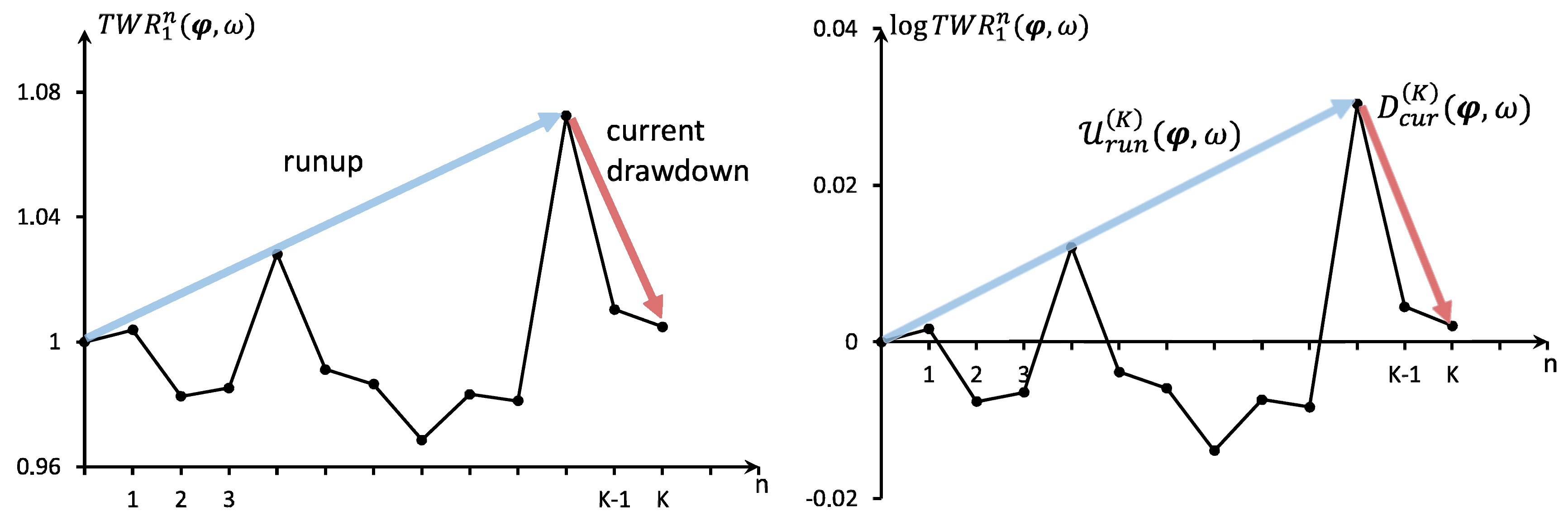
5. The Current Drawdown

Several authors have already investigated drawdown related risk measures, focusing mostly on the absolute drawdown (see references Chekhlov et al. (2003, 2005); Goldberg and Mahmoud (2017); Zabarankin et al. (2014)). However, absolute drawdowns are problematic, in particular when long time series are observed, because then prices often vary over big ranges. We, therefore, took a different approach and constructed a drawdown related risk measure from relative drawdowns. Whereas the absolute drawdown measures the absolute price difference between the historic high points and the current price, the relative drawdown measures the percentage loss between the these two prices.

We keep discussing the trading return matrix T from (1) and probabilities $p_1,\dots ,p_N$ from Setup 1 for each row ${\mathit{t}}_{i\mathbf{·}}$ of T. Drawing randomly and independently $K\in \mathbb{N}$ times such rows from that distribution results in a terminal wealth relative for fractional trading

$$\begin{array}{c}\hfill {\mathrm{TWR}}_1^K(\mathit{\phi },\omega )=\prod _{j=1}^K\left(1+\langle {\mathit{t}}_{{\omega }_j\mathbf{·}}^{\mathsf{\top }},\mathit{\phi }\rangle \right),\mathit{\phi }\in \stackrel{\circ }{\mathfrak{G}},\omega \in {\Omega }^{\left(K\right)}={\left\{1,\dots ,N\right\}}^K,\end{array}$$

depending on the betted portions, $\mathit{\phi }=\left({\phi }_1,\dots ,{\phi }_M\right)$ (see Equation (8)). In order to investigate the current drawdown realized after the K-th draw, we more generally use the notation

$$\begin{array}{c}\hfill {\mathrm{TWR}}_m^n(\mathit{\phi },\omega ):=\prod _{j=m}^n\left(1+\langle {\mathit{t}}_{{\omega }_j\mathbf{·}}^{\mathsf{\top }},\mathit{\phi }\rangle \right).\end{array}$$

(44)

The idea here is that ${\mathrm{TWR}}_1^n(\mathit{\phi },\omega )$ is viewed as a discrete “equity curve” at time n (with $\mathit{\phi }$ and ω fixed). The current drawdown log series is defined as the logarithm of the drawdown of this equity curve realized from the maximum of the curve till the end (time K). We show below that this series is the counterpart of the run–up (cf. Figure 4).

Definition 6.

The current drawdown log series is set to

$$\begin{array}{c}\hfill {\mathcal{D}}_{\mathrm{cur}}^{\left(K\right)}(\mathit{\phi },\omega ):=\ln \left(\underset{1\le \ell \le K}{\min }\min \{1,{\mathrm{TWR}}_{\ell }^K(\mathit{\phi },\omega )\}\right)\le 0,\end{array}$$

(45)

and the run-up log series is defined as

$$\begin{array}{c}\hfill {\mathcal{U}}_{\mathrm{run}}^{\left(K\right)}(\mathit{\phi },\omega ):=\ln \left(\underset{1\le \ell \le K}{\max }\max \{1,{\mathrm{TWR}}_1^{\ell }(\mathit{\phi },\omega )\}\right)\ge 0.\end{array}$$

The corresponding trade series are connected because the current drawdown starts after the run-up has stopped. To make this more precise, we fix ℓ where the run-up reaches its top.

Definition 7.

(first TWR topping point) For fixed $\omega \in {\Omega }^{\left(K\right)}$ and $\mathit{\phi }\in \stackrel{\circ }{\mathfrak{G}}$, define ${\ell }^{*}={\ell }^{*}(\mathit{\phi },\omega )\in \{0,\dots ,K\}$ with

(a) 

${\ell }^{*}=0$ in case $\underset{1\le \ell \le K}{\max }{\mathrm{TWR}}_1^{\ell }(\mathit{\phi },\omega )\le 1$

(b) 

and otherwise, choose ${\ell }^{*}\in \{1,\dots ,K\}$ such that

$$\begin{array}{c}\hfill {\mathrm{TWR}}_1^{{\ell }^{*}}(\mathit{\phi },\omega )=\underset{1\le \ell \le K}{\max }{\mathrm{TWR}}_1^{\ell }(\mathit{\phi },\omega )>1,\end{array}$$

(46)

where ${\ell }^{*}$ should be minimal with that property.

By definition, one easily gets

$$\begin{array}{cc}\hfill {\mathcal{D}}_{\mathrm{cur}}^{\left(K\right)}(\mathit{\phi },\omega )& =\left\{\begin{array}{cc}\ln {\mathrm{TWR}}_{{\ell }^{*}+1}^K(\mathit{\phi },\omega ),\hfill & \mathrm{in}\mathrm{case}{\ell }^{*}<K,\hfill \\ 0,\hfill & \mathrm{in}\mathrm{case}{\ell }^{*}=K,\hfill \end{array}\right.\hfill \end{array}$$

(47)

and

$$\begin{array}{cc}\hfill {\mathcal{U}}_{\mathrm{run}}^{\left(K\right)}(\mathit{\phi },\omega )& =\left\{\begin{array}{cc}\ln {\mathrm{TWR}}_1^{{\ell }^{*}}(\mathit{\phi },\omega ),\hfill & \mathrm{in}\mathrm{case}{\ell }^{*}\ge 1,\hfill \\ 0,\hfill & \mathrm{in}\mathrm{case}{\ell }^{*}=0.\hfill \end{array}\right.\hfill \end{array}$$

(48)

As in Section 3, we immediately obtain ${\mathcal{D}}_{\mathrm{cur}}^{\left(K\right)}(\mathit{\phi },\omega )+{\mathcal{U}}_{\mathrm{run}}^{\left(K\right)}(\mathit{\phi },\omega )={\mathcal{Z}}^{\left(K\right)}(\mathit{\phi },\omega )$ and therefore, by Theorem 1,

Corollary 3.

For $\mathit{\phi }\in \stackrel{\circ }{\mathfrak{G}}$,

$$\begin{array}{c}\hfill \mathbb{E}\left[{\mathcal{D}}_{\mathrm{cur}}^{\left(K\right)}(\mathit{\phi },·)\right]+\mathbb{E}\left[{\mathcal{U}}_{\mathrm{run}}^{\left(K\right)}(\mathit{\phi },·)\right]=K·\ln \Gamma \left(\mathit{\phi }\right)\end{array}$$

(49)

holds.

Explicit formulas for the expectation of ${\mathcal{D}}_{\mathrm{cur}}^{\left(K\right)}$ and ${\mathcal{U}}_{\mathrm{run}}^{\left(K\right)}$ are again of interest. By definition and with (47),

$$\begin{array}{c}\hfill \mathbb{E}\left[{\mathcal{D}}_{\mathrm{cur}}^{\left(K\right)}(\mathit{\phi },·)\right]=\sum _{\ell =0}^{K-1}\sum _{\begin{array}{c}\omega \in {\Omega }^{\left(K\right)}\\ {\ell }^{*}(\mathit{\phi },\omega )=\ell \end{array}}\mathbb{P}\left(\left\{\omega \right\}\right)·\ln {\mathrm{TWR}}_{\ell +1}^K\left(\mathit{\phi },\omega \right).\end{array}$$

(50)

Before we proceed with this calculation, we need to discuss ${\ell }^{*}={\ell }^{*}\left(\mathit{\phi },\omega \right)$ further for some fixed ω. From Definition 7, in case ${\ell }^{*}\ge 1$, we get

$$\begin{array}{cc}\hfill {\mathrm{TWR}}_k^{{\ell }^{*}}\left(\mathit{\phi },\omega \right)& >1\mathrm{for}k=1,\dots ,{\ell }^{*},\hfill \end{array}$$

(51)

since ${\ell }^{*}$ is the first time the run-up is topped, and, in case ${\ell }^{*}<K$,

$$\begin{array}{cc}\hfill {\mathrm{TWR}}_{{\ell }^{*}+1}^{\tilde{k}}\left(\mathit{\phi },\omega \right)& \le 1\mathrm{for}\tilde{k}={\ell }^{*}+1,\dots ,K.\hfill \end{array}$$

(52)

Similarly to Section 3, we write $\mathit{\phi }\ne 0$ as $\mathit{\phi }=s\mathit{\theta }$ for $\mathit{\theta }\in {\mathbb{S}}_1^{M-1}$ and $s>0$. The last inequality then may be rephrased for $s\in (0,\epsilon ]$ and some sufficiently small $\epsilon >0$ as

$$\begin{array}{cc}\hfill {\mathrm{TWR}}_{{\ell }^{*}+1}^{\tilde{k}}(s\mathit{\theta },\omega )\le 1& ⟺\ln {\mathrm{TWR}}_{{\ell }^{*}+1}^{\tilde{k}}((s\mathit{\theta },\omega )\le 0\hfill \\ \hfill & ⟺\sum _{j={\ell }^{*}+1}^{\tilde{k}}\ln \left(1+s\langle {\mathit{t}}_{{\omega }_j\mathbf{·}}^{\mathsf{\top }},\mathit{\theta }\rangle \right)\le 0\hfill \\ \hfill & ⟺\sum _{j={\ell }^{*}+1}^{\tilde{k}}\langle {\mathit{t}}_{{\omega }_j\mathbf{·}}^{\mathsf{\top }},\mathit{\theta }\rangle \le 0\hfill \end{array}$$

(53)

by an argument similar to Lemma 3. Analogously, one finds for all $s\in (0,\epsilon ]$

$$\begin{array}{c}\hfill {\mathrm{TWR}}_k^{{\ell }^{*}}(s\mathit{\theta },\omega )>1⟺\sum _{j=k}^{{\ell }^{*}}\langle {\mathit{t}}_{{\omega }_j\mathbf{·}}^{\mathsf{\top }},\mathit{\theta }\rangle >0.\end{array}$$

(54)

This observation will become crucial to proof the next result on the expectation of the current drawdown.

Theorem 6.

Let a trading game as in Setup 1 with $N,K\in \mathbb{N}$ be fixed. Then, for $\mathit{\theta }\in {\mathbb{S}}_1^{M-1}$ and $s\in (0,\epsilon ]$, the following holds:

$$\begin{array}{c}\hfill \mathbb{E}\left[{\mathcal{D}}_{\mathrm{cur}}^{\left(K\right)}(s\mathit{\theta },·)\right]=d_{cur}^{\left(K\right)}(s,\mathit{\theta }):=\sum _{n=1}^N\left(\sum _{\ell =0}^K{\Lambda }_n^{(\ell ,K,N)}\left(\mathit{\theta }\right)\right)·\ln \left(1+s\langle {\mathit{t}}_{n\mathbf{·}}^{\mathsf{\top }},\mathit{\theta }\rangle \right)\end{array}$$

(55)

where ${\Lambda }_n^{(K,K,N)}:=0$ is independent of $\mathit{\theta }$ and for $\ell \in \{0,1,\dots ,K-1\}$, the functions ${\Lambda }_n^{(\ell ,K,N)}\left(\mathit{\theta }\right)\ge 0$ are defined by

$$\begin{array}{c}\hfill {\Lambda }_n^{(\ell ,K,N)}\left(\mathit{\theta }\right):=\sum _{\begin{array}{c}\omega \in {\Omega }^{\left(K\right)}\\ {\displaystyle \sum _{j=k}^{\ell }}\langle {\mathit{t}}_{{\omega }_j\mathbf{·}}^{\mathsf{\top }},\mathit{\theta }\rangle >0fork=1,\dots ,\ell \\ {\displaystyle \sum _{j=\ell +1}^{\tilde{k}}}\langle {\mathit{t}}_{{\omega }_j\mathbf{·}}^{\mathsf{\top }},\mathit{\theta }\rangle \le 0for\tilde{k}=\ell +1,\dots ,K\end{array}}\mathbb{P}\left(\left\{\omega \right\}\right)·\#\left\{i|{\omega }_i=n,i\ge \ell +1\right\}.\end{array}$$

(56)

Proof. 

Again, the proof is very similar to the proof in the univariate case (see Theorem 5.4 in Maier-Paape (2018)). Starting with (50), we get

$$\begin{array}{c}\hfill \mathbb{E}\left[{\mathcal{D}}_{\mathrm{cur}}^{\left(K\right)}(s\mathit{\theta },·)\right]=\sum _{\ell =0}^{K-1}\sum _{\begin{array}{c}\omega \in {\Omega }^{\left(K\right)}\\ {\ell }^{*}(s\mathit{\theta },\omega )=\ell \end{array}}\mathbb{P}\left(\left\{\omega \right\}\right)·\sum _{i=\ell +1}^K\ln \left(1+\langle {\mathit{t}}_{{\omega }_i\mathbf{·}}^{\mathsf{\top }},s\mathit{\theta }\rangle \right)\end{array}$$

and by (53) and (54) for all $s\in (0,\epsilon ]$,

$$\begin{array}{c}\mathbb{E}\left[{\mathcal{D}}_{\mathrm{cur}}^{\left(K\right)}(s\mathit{\theta },·)\right]=\sum _{\ell =0}^{K-1}\sum _{\begin{array}{c}\omega \in {\Omega }^{\left(K\right)}\\ {\displaystyle \sum _{j=k}^{\ell }}\langle {\mathit{t}}_{{\omega }_j\mathbf{·}}^{\mathsf{\top }},\mathit{\theta }\rangle >0\mathrm{for}k=1,\dots ,\ell \\ {\displaystyle \sum _{j=\ell +1}^{\tilde{k}}}\langle {\mathit{t}}_{{\omega }_j\mathbf{·}}^{\mathsf{\top }},\mathit{\theta }\rangle \le 0\mathrm{for}\tilde{k}=\ell +1,\dots ,K\end{array}}\mathbb{P}\left(\left\{\omega \right\}\right)·\sum _{i=\ell +1}^K\ln \left(1+s\langle {\mathit{t}}_{{\omega }_i\mathbf{·}}^{\mathsf{\top }},\mathit{\theta }\rangle \right)\hfill \\ =\sum _{\ell =0}^{K-1}\sum _{\begin{array}{c}\omega \in {\Omega }^{\left(K\right)}\\ {\displaystyle \sum _{j=k}^{\ell }}\langle {\mathit{t}}_{{\omega }_j\mathbf{·}}^{\mathsf{\top }},\mathit{\theta }\rangle >0\mathrm{for}k=1,\dots ,\ell \\ {\displaystyle \sum _{j=\ell +1}^{\tilde{k}}}\langle {\mathit{t}}_{{\omega }_j\mathbf{·}}^{\mathsf{\top }},\mathit{\theta }\rangle \le 0\mathrm{for}\tilde{k}=\ell +1,\dots ,K\end{array}}\mathbb{P}\left(\left\{\omega \right\}\right)·\sum _{n=1}^N\#\left\{i|{\omega }_i=n,i\ge \ell +1\right\}·\ln \left(1+s\langle {\mathit{t}}_{n\mathbf{·}}^{\mathsf{\top }},\mathit{\theta }\rangle \right)\hfill \\ =\sum _{n=1}^N\sum _{\ell =0}^{K-1}{\Lambda }_n^{(\ell ,K,N)}\left(\mathit{\theta }\right)·\ln \left(1+s\langle {\mathit{t}}_{n\mathbf{·}}^{\mathsf{\top }},\mathit{\theta }\rangle \right)=d_{\mathrm{cur}}^{\left(K\right)}(s,\mathit{\theta })\hfill \end{array}$$

(57)

since ${\Lambda }_n^{(K,K,N)}=0$. ☐

In order to simplify the notation, we formally introduce the “linear equity curve" for $1\le m\le n\le K,\omega \in {\Omega }^{\left(K\right)}={\left\{1,\dots ,N\right\}}^K$ and $\mathit{\theta }\in {\mathbb{S}}_1^{M-1}$:

$$\begin{array}{c}\hfill {\mathrm{linEQ}}_m^n(\mathit{\theta },\omega ):=\sum _{j=m}^n\langle {\mathit{t}}_{{\omega }_j\mathbf{·}}^{\mathsf{\top }},\mathit{\theta }\rangle \end{array}$$

(58)

Then, we obtain, similarly to the first topping point ${\ell }^{*}={\ell }^{*}(\mathit{\phi },\omega )$ of the TWR-equity curve (44) (cf. Definition 7), the first topping point for the linear equity:

Definition 8.

(first linear equity topping point) For fixed $\omega \in {\Omega }^{\left(K\right)}$ and $\mathit{\theta }\in {\mathbb{S}}_1^{M-1}$ define ${\widehat{\ell }}^{*}={\widehat{\ell }}^{*}(\mathit{\theta },\omega )\in \{0,\dots ,K\}$ with

(a) 

${\widehat{\ell }}^{*}=0$ in case $\underset{1\le \ell \le K}{\max }{\mathrm{linEQ}}_1^{\ell }(\mathit{\theta },\omega )\le 0$

(b) 

and otherwise, choose ${\widehat{\ell }}^{*}\in \{1,\dots ,K\}$ such that

$$\begin{array}{c}\hfill {\mathrm{linEQ}}_1^{{\widehat{\ell }}^{*}}(\mathit{\theta },\omega )=\underset{1\le \ell \le K}{\max }{\mathrm{linEQ}}_1^{\ell }(\mathit{\theta },\omega )>0,\end{array}$$

(59)

where ${\widehat{\ell }}^{*}$ should be minimal with that property.

Let us discuss ${\widehat{\ell }}^{*}={\widehat{\ell }}^{*}(\mathit{\theta },\omega )$ further for some fixed ω. From Definition 8, in case ${\widehat{\ell }}^{*}\ge 1$, we get

$$\begin{array}{c}\hfill {\mathrm{linEQ}}_k^{{\widehat{\ell }}^{*}}(\mathit{\theta },\omega )>0\mathrm{for}k=1,\dots ,{\widehat{\ell }}^{*}\end{array}$$

(60)

since ${\widehat{\ell }}^{*}$ is the first time that the run-up of the linear equity has been topped and, in case ${\widehat{\ell }}^{*}<K$

$$\begin{array}{c}\hfill {\mathrm{linEQ}}_{{\widehat{\ell }}^{*}+1}^{\tilde{k}}(\mathit{\theta },\omega )\le 0\mathrm{for}\tilde{k}={\widehat{\ell }}^{*}+1,\dots ,K.\end{array}$$

(61)

Hence, we conclude that $\omega \in {\Omega }^{\left(K\right)}$ satisfies ${\widehat{\ell }}^{*}(\mathit{\theta },\omega )=\ell$ if and only if

$$\begin{array}{c}\hfill \sum _{j=k}^{\ell }\langle {\mathit{t}}_{{\omega }_j\mathbf{·}}^{\mathsf{\top }},\mathit{\theta }\rangle >0\mathrm{for}k=1,\dots ,\ell \mathrm{and}\sum _{j=\ell +1}^{\tilde{k}}\langle {\mathit{t}}_{{\omega }_j\mathbf{·}}^{\mathsf{\top }},\mathit{\theta }\rangle \le 0\mathrm{for}\tilde{k}=\ell +1,\dots ,K.\end{array}$$

(62)

Therefore, (56) simplifies to

$$\begin{array}{c}\hfill {\Lambda }_n^{(\ell ,K,N)}\left(\mathit{\theta }\right)=\sum _{\begin{array}{c}\omega \in {\Omega }^{\left(K\right)}\\ {\widehat{\ell }}^{*}(\mathit{\theta },\omega )=\ell \end{array}}\mathbb{P}\left(\left\{\omega \right\}\right)·\#\left\{i|{\omega }_i=n,i\ge \ell +1\right\}.\end{array}$$

(63)

Furthermore, according to (53) and (54), for small $s>0$, ${\ell }^{*}\mathrm{ad}{\widehat{\ell }}^{*}$ coincide, i.e.,

$$\begin{array}{c}\hfill {\widehat{\ell }}^{*}(\mathit{\theta },\omega )={\ell }^{*}(s\mathit{\theta },\omega )\mathrm{for}\mathrm{all}s\in (0,\epsilon ].\end{array}$$

(64)

A very similar argument to the proof of Theorem 6 yields

Theorem 7.

In the situation of Theorem 6, for $\mathit{\theta }\in {\mathbb{S}}_1^{M-1}$ and all $s\in (0,\epsilon ]$,

$$\begin{array}{c}\hfill \mathbb{E}\left[{\mathcal{U}}_{\mathrm{run}}^{\left(K\right)}(s\mathit{\theta },·)\right]=u_{\mathrm{run}}^{\left(K\right)}(s,\mathit{\theta }):=\sum _{n=1}^N\left(\sum _{\ell =0}^K{\mathsf{{\rm Y}}}_n^{(\ell ,K,N)}\left(\mathit{\theta }\right)\right)·\ln \left(1+s\langle {\mathit{t}}_{n·}^{\mathsf{\top }},\mathit{\theta }\rangle \right)\end{array}$$

(65)

holds, where ${\mathsf{{\rm Y}}}_n^{(0,K,N)}:=0$ is independent from $\mathit{\theta }$ and for $\ell \in \{1,\dots ,K\}$, the functions ${\mathsf{{\rm Y}}}_n^{(\ell ,K,N)}\left(\mathit{\theta }\right)\ge 0$ are given as

$$\begin{array}{c}\hfill {\mathsf{{\rm Y}}}_n^{(\ell ,K,N)}\left(\mathit{\theta }\right):=\sum _{\begin{array}{c}\omega \in {\Omega }^{\left(K\right)}\\ {\widehat{\ell }}^{*}(\mathit{\theta },\omega )=\ell \end{array}}\mathbb{P}\left(\left\{\omega \right\}\right)·\#\left\{i|{\omega }_i=n,i\le \ell \right\}.\end{array}$$

(66)

Remark 11.

Again, we immediately obtain a first-order approximation for the expected current drawdown log series. For $s\in (0,\epsilon ]$,

$$\begin{array}{c}\hfill \mathbb{E}\left[{\mathcal{D}}_{\mathrm{cur}}^{\left(K\right)}(s\mathit{\theta },·)\right]\approx {\tilde{d}}_{\mathrm{cur}}^{\left(K\right)}(s,\mathit{\theta }):=s·\sum _{n=1}^N\left(\sum _{\ell =0}^K{\Lambda }_n^{\left(\ell ,K,N\right)}\left(\mathit{\theta }\right)\right)·\langle {\mathit{t}}_{n\mathbf{·}}^{\mathsf{\top }},\mathit{\theta }\rangle \end{array}$$

(67)

holds. Moreover, since ${\mathcal{D}}_{\mathrm{cur}}^{\left(K\right)}(\mathit{\phi },\omega )\le {\mathcal{D}}^{\left(K\right)}(\mathit{\phi },\omega )\le 0,d_{\mathrm{cur}}^{\left(K\right)}(s,\mathit{\theta })\le d^{\left(K\right)}(s,\mathit{\theta })\le 0$ and ${\tilde{d}}_{\mathrm{cur}}^{\left(K\right)}(s,\mathit{\theta })\le {\tilde{d}}^{\left(K\right)}(s,\mathit{\theta })\le 0$ holds as well.

As discussed in Section 4 for the down-trade log series, we also want to study the current drawdown log series (45) with respect to admissible convex risk measures.

Theorem 8.

For a trading game as in Setup 1 satisfying Assumption 1, the function ${\mathfrak{r}}_{\mathrm{cur}}:\stackrel{\circ }{\mathfrak{G}}\to {\mathbb{R}}_0^{+}$,

$$\begin{array}{c}\hfill {\mathfrak{r}}_{\mathrm{cur}}\left(\mathit{\phi }\right)={\mathfrak{r}}_{\mathrm{cur}}^{\left(K\right)}\left(\mathit{\phi }\right):=-\mathbb{E}\left[{\mathcal{D}}_{\mathrm{cur}}^{\left(K\right)}(\mathit{\phi },·)\right]\ge 0,\mathit{\phi }\in \stackrel{\circ }{\mathfrak{G}},\end{array}$$

(68)

is an admissible convex risk measure (ACRM).

Proof. 

It is easy to see that the proof of Theorem 4 can almost literally be adapted to the current drawdown case. ☐

Regard Figure 5 for an illustration of ${\mathfrak{r}}_{\mathrm{cur}}$. Compared to ${\mathfrak{r}}_{\mathrm{down}}$ in Figure 1 the contour plot looks quite similar, but near $0\in {\mathbb{R}}^M$, obviously, ${\mathfrak{r}}_{\mathrm{cur}}$ grows faster. Similarly, we obtain an ACRM for the first-order approximation ${\tilde{d}}_{\mathrm{cur}}^{\left(K\right)}(s,\mathit{\theta })$ in (67):

Theorem 9.

For the trading game of Setup 1 satisfying Assumption 1, the function ${\mathfrak{r}}_{\mathrm{cur}X}:{\mathbb{R}}^M\to {\mathbb{R}}_0^{+}$,

$$\begin{array}{c}\hfill {\mathfrak{r}}_{\mathrm{cur}X}\left(\mathit{\phi }\right)={\mathfrak{r}}_{\mathrm{cur}X}^{\left(K\right)}\left(s\mathit{\theta }\right):=-{\tilde{d}}_{\mathrm{cur}}^{\left(K\right)}(s,\mathit{\theta })=-s·L_{\mathrm{cur}}^{(K,N)}\left(\mathit{\theta }\right)\ge 0,fors\ge 0and\mathit{\theta }\in {\mathbb{S}}_1^{M-1}\end{array}$$

with

$$\begin{array}{cc}& L_{\mathrm{cur}}^{(K,N)}\left(\mathit{\theta }\right):=\sum _{\ell =0}^{K-1}\sum _{\begin{array}{c}\omega \in {\Omega }^{\left(K\right)}\\ {\widehat{\ell }}^{*}(\mathit{\theta },\omega )=\ell \end{array}}\mathbb{P}\left(\left\{\omega \right\}\right)·\sum _{i=\ell +1}^K\langle {\mathit{t}}_{{\omega }_i·}^{\mathsf{\top }},\mathit{\theta }\rangle \hfill \end{array}$$

(69)

is an admissible convex risk measure (ACRM) according to Definition 3 which is moreover positive homogeneous.

Proof. 

We use (57) to derive the above formula for $L_{\mathrm{cur}}^{(K,N)}\left(\mathit{\theta }\right)$. Now, most of the arguments of the proof of Theorem 5 work here as well, once we know that $L_{\mathrm{cur}}^{(K,N)}\left(\mathit{\theta }\right)$ is continuous in $\mathit{\theta }$. To see that, we remark once more that for the first topping point, ${\widehat{\ell }}^{*}={\widehat{\ell }}^{*}(\mathit{\theta },\omega )\in \{0,\dots ,K\}$, of the linearized equity curve ${\sum }_{j=1}^n\langle {\mathit{t}}_{{\omega }_j·}^{\mathsf{\top }},\mathit{\theta }\rangle ,n=1,\dots ,K$, the following holds (cf. Definition 8 and (61)):

$$\begin{array}{c}\hfill {\mathrm{linEQ}}_{{\widehat{\ell }}^{*}+1}^K(\mathit{\theta },\omega )=\sum _{i={\widehat{\ell }}^{*}+1}^K\langle {\mathit{t}}_{{\omega }_i·}^{\mathsf{\top }},\mathit{\theta }\rangle \le 0.\end{array}$$

Thus,

$$\begin{array}{c}{L}_{\mathrm{cur}}^{(K,N)}\left(\mathit{\theta }\right)=\sum _{\ell =0}^{K-1}\sum _{\begin{array}{c}\omega \in {\Omega }^{\left(K\right)}\\ {\widehat{\ell }}^{*}(\mathit{\theta },\omega )=\ell \end{array}}\mathbb{P}\left(\left\{\omega \right\}\right)·\underset{\le 0}{\underbrace{\sum _{i=\ell +1}^K\langle {\mathit{t}}_{{\omega }_i\mathbf{·}}^{\mathsf{\top }},\mathit{\theta }\rangle }}\le 0.\hfill \end{array}$$

Although the topping point ${\widehat{\ell }}^{*}(\mathit{\theta },\omega )$ for $\omega \in {\Omega }^{\left(K\right)}$ may jump when $\mathit{\theta }$ is varied in case ${\sum }_{i={\widehat{\ell }}^{*}+1}^j\langle {\mathit{t}}_{{\omega }_i\mathbf{·}}^{\mathsf{\top }},\mathit{\theta }\rangle =0$ for some $j\ge {\widehat{\ell }}^{*}+1$, i.e.,

$$\begin{array}{c}\hfill \sum _{i={\widehat{\ell }}^{*}+1}^K\langle {\mathit{t}}_{{\omega }_i\mathbf{·}}^{\mathsf{\top }},\mathit{\theta }\rangle =\sum _{i=j}^K\langle {\mathit{t}}_{{\omega }_i\mathbf{·}}^{\mathsf{\top }},\mathit{\theta }\rangle ,\end{array}$$

the continuity of $L_{\mathrm{cur}}^{(K,N)}\left(\mathit{\theta }\right)$ is still granted since the summation is over all $\ell =0,\dots ,K-1$. Hence, all claims are proved. ☐

A contour plot of ${\mathfrak{r}}_{\mathrm{cur}X}$ can be seen in Figure 6. The first topping point of the linearized equity curve will also be helpful to order the risk measures ${\mathfrak{r}}_{\mathrm{cur}}$ and ${\mathfrak{r}}_{\mathrm{cur}X}$. Reasoning as in (53) (see also Lemma 3) and using (61), we obtain, in case ${\widehat{\ell }}^{*}<K$ for $s\in (0,\epsilon ]$ and $\tilde{k}={\widehat{\ell }}^{*}+1,\dots ,K$, that

$$\begin{array}{c}\hfill {\mathrm{linEQ}}_{{\widehat{\ell }}^{*}+1}^{\tilde{k}}(\mathit{\theta },\omega )=\sum _{j={\widehat{\ell }}^{*}+1}^{\tilde{k}}\langle {\mathit{t}}_{{\omega }_j\mathbf{·}}^{\mathsf{\top }},\mathit{\theta }\rangle \le 0⟹\sum _{j={\widehat{\ell }}^{*}+1}^{\tilde{k}}\ln \left(1+s\langle {\mathit{t}}_{{\omega }_j\mathbf{·}}^{\mathsf{\top }},\mathit{\theta }\rangle \right)\le 0.\end{array}$$

(70)

However, since ln is concave, the above implication holds true even for all $s>0$ with $\mathit{\phi }=s\mathit{\theta }\in \stackrel{\circ }{\mathfrak{G}}$. Hence, for $\tilde{k}={\widehat{\ell }}^{*}+1,\dots ,K$ and $\mathit{\phi }=s\mathit{\theta }\in \stackrel{\circ }{\mathfrak{G}}$

$$\begin{array}{c}\hfill {\mathrm{linEQ}}_{{\widehat{\ell }}^{*}+1}^{\tilde{k}}(\mathit{\theta },\omega )\le 0⟹\ln {\mathrm{TWR}}_{{\widehat{\ell }}^{*}+1}^{\tilde{k}}(s\mathit{\theta },\omega )\le 0.\end{array}$$

(71)

Looking at (52) once more, we observe that the first topping point of the TWR equity curve ${\ell }^{*}$ necessarily is less than or equal to ${\widehat{\ell }}^{*}$. Thus, we have shown

Lemma 6.

For all $\omega \in {\Omega }^{\left(K\right)}$ and $\mathit{\phi }=s\mathit{\theta }\in \stackrel{\circ }{\mathfrak{G}}$ the following holds (see also (64)):

$$\begin{array}{c}\hfill {\ell }^{*}(s\mathit{\theta },\omega )\le {\widehat{\ell }}^{*}(\mathit{\theta },\omega ).\end{array}$$

(72)

This observation helps to order $\mathbb{E}\left[{\mathcal{D}}_{\mathrm{cur}}^{\left(K\right)}(s\mathit{\theta },·)\right]$ and $d_{\mathrm{cur}}^{\left(K\right)}(s,\mathit{\theta })$:

Theorem 10.

For all $\mathit{\phi }=s\mathit{\theta }\in \stackrel{\circ }{\mathfrak{G}}$, with $s>0$ and $\mathit{\theta }\in {\mathbb{S}}_1^{M-1}$, we have

$$\begin{array}{c}\hfill \mathbb{E}\left[{\mathcal{D}}_{\mathrm{cur}}^{\left(K\right)}(s\mathit{\theta },·)\right]\le d_{\mathrm{cur}}^{\left(K\right)}(s,\mathit{\theta })\le {\tilde{d}}_{\mathrm{cur}}^{\left(K\right)}(s,\mathit{\theta })\le 0.\end{array}$$

(73)

Proof. 

Using (50) for $\mathit{\phi }=s\mathit{\theta }\in \stackrel{\circ }{\mathfrak{G}}$,

$$\begin{array}{c}\hfill \begin{array}{ccc}\hfill {\displaystyle \mathbb{E}\left[{\mathcal{D}}_{\mathrm{cur}}^{\left(K\right)}(s\mathit{\theta },·)\right]}& =& {\displaystyle \sum _{\ell =0}^{K-1}\sum _{\begin{array}{c}\omega \in {\Omega }^{\left(K\right)}\\ {\ell }^{*}(s\mathit{\theta },\omega )=\ell \end{array}}\mathbb{P}\left(\left\{\omega \right\}\right)·\ln {\mathrm{TWR}}_{\ell +1}^K(s\mathit{\theta },\omega )}\hfill \\ & \stackrel{\mathrm{Lemma}6}{\le }& {\displaystyle \sum _{\ell =0}^{K-1}\sum _{\begin{array}{c}\omega \in {\Omega }^{\left(K\right)}\\ {\widehat{\ell }}^{*}(\mathit{\theta },\omega )=\ell \end{array}}\mathbb{P}\left(\left\{\omega \right\}\right)·\sum _{i=\ell +1}^K\ln \left(1+s\langle {\mathit{t}}_{{\omega }_i\mathbf{·}}^{\mathsf{\top }},\mathit{\theta }\rangle \right)}\hfill \\ & \stackrel{\left(62\right)}{=}& \hfill {\displaystyle \sum _{\ell =0}^{K-1}\sum _{\begin{array}{c}\omega \in {\Omega }^{\left(K\right)}\\ {\displaystyle \sum _{j=k}^{\ell }}\langle {\mathit{t}}_{{\omega }_j\mathbf{·}}^{\mathsf{\top }},\mathit{\theta }\rangle >0\mathrm{for}k=1,\dots ,\ell \\ {\displaystyle \sum _{j=\ell +1}^{\tilde{k}}}\langle {\mathit{t}}_{{\omega }_j\mathbf{·}}^{\mathsf{\top }},\mathit{\theta }\rangle \le 0\mathrm{for}\tilde{k}=\ell +1,\dots ,K\end{array}}\mathbb{P}\left(\left\{\omega \right\}\right)·\sum _{i=\ell +1}^K\ln \left(1+s\langle {\mathit{t}}_{{\omega }_i\mathbf{·}}^{\mathsf{\top }},\mathit{\theta }\rangle \right)\stackrel{\left(57\right)}{=}{d}_{\mathrm{cur}}^{\left(K\right)}(s,\mathit{\theta }).}\end{array}\end{array}$$

The second inequality in (73) follows, as in Section 3, from $\ln (1+x)\le x$ (see (55) and (67)) and the third inequality is already clear from Remark 11. ☐

6. Conclusions

Let us summarize the results of the last sections. We obtained two down-trade log series related admissible convex risk measures (ACRM) according to Definition 3, namely

$$\begin{array}{c}\hfill {\mathfrak{r}}_{\mathrm{down}}\left(\mathit{\phi }\right)\ge {\mathfrak{r}}_{\mathrm{down}X}\left(\mathit{\phi }\right)\ge 0\mathrm{for}\mathrm{all}\mathit{\phi }\in \stackrel{\circ }{\mathfrak{G}}\end{array}$$

(see Corollary 2 and Theorems 4 and 5). Similarly, we obtained two current drawdown-related (ACRM), namely,

$$\begin{array}{c}\hfill {\mathfrak{r}}_{\mathrm{cur}}\left(\mathit{\phi }\right)\ge {\mathfrak{r}}_{\mathrm{cur}X}\left(\mathit{\phi }\right)\ge 0\mathrm{for}\mathrm{all}\mathit{\phi }\in \stackrel{\circ }{\mathfrak{G}}\end{array}$$

(cf. Theorems 8 and 9 as well as Theorem 10). Furthermore, due to Remark 11, we have the ordering

$$\begin{array}{c}\hfill {\mathfrak{r}}_{\mathrm{cur}}\left(\mathit{\phi }\right)\ge {\mathfrak{r}}_{\mathrm{down}}\left(\mathit{\phi }\right)\mathrm{and}{\mathfrak{r}}_{\mathrm{cur}X}\left(\mathit{\phi }\right)\ge {\mathfrak{r}}_{\mathrm{down}X}\left(\mathit{\phi }\right),\mathit{\phi }\in \stackrel{\circ }{\mathfrak{G}}.\end{array}$$

(74)

All four risk measures can be used in order to apply the general framework for the portfolio theory of reference Maier-Paape and Zhu (2018). Since the two approximated risk measures ${\mathfrak{r}}_{\mathrm{down}X}$ and ${\mathfrak{r}}_{\mathrm{cur}X}$ are positive homogeneous, according to reference Maier-Paape and Zhu (2018), the efficient portfolios will have an affine linear structure. Although we were able to prove a lot of results for these for practical applications relevant risk measures, there are still open questions. To state only one of them, we note that convergence of these risk measures for $K\to \infty$ is unclear, but empirical evidence seems to support such a statement (see Figure 7).

Furthermore, a variety of real-world applications should be discussed in order to verify the practical benefit of portfolios constructed with drawdown risk measures. We intend to do this in future work.

References

1. Chekhlov, Alexei, Stanislav Uryasev, and Michael Zabarankin. 2003. Portfolio optimization with drawdown constraints. In Asset and Liability Management Tools. Edited by Bernd Scherer. London: Risk Books, pp. 263–78. [Google Scholar]
2. Chekhlov, Alexei, Stanislav Uryasev, and Michael Zabarankin. 2005. Drawdown measure in portfolio optimization. International Journal of Theoretical and Applied Finance 8: 13–58. [Google Scholar] [CrossRef]
3. Föllmer, Hans, and Alexander Schied. 2002. Stochastic Finance, 1st ed. Berlin: De Gruyter. [Google Scholar]
4. Goldberg, Lisa R., and Ola Mahmoud. 2017. Drawdown: from Practice to Theory and Back Again. Mathematics and Financial Economics 11: 275–97. [Google Scholar] [CrossRef]
5. Hermes, Andreas. 2016. A Mathematical Approach to Fractional Trading: Using the Terminal Wealth Relative with Discrete and Continuous Distributions. Ph.D. thesis, RWTH Aachen University, Aachen, Germany. [Google Scholar] [CrossRef]
6. Hermes, Andreas, and Stanislaus Maier-Paape. 2017. Existence and uniqueness for the multivariate discrete terminal wealth relative. Risks 5: 44. [Google Scholar] [CrossRef]
7. Kelly, John L., Jr. 1956. A new interpretation of information rate. Bell System Technical Journal 35: 917–26. [Google Scholar] [CrossRef]
8. Maier-Paape, Stanislaus. 2013. Existence Theorems for Optimal Fractional Trading. Report No. 67. Aachen: Institut für Mathematik, RWTH Aachen University, Available online: https://www.instmath.rwth-aachen.de/Preprints/maierpaape20131008.pdf (accessed on 6 August 2018).
9. Maier-Paape, Stanislaus. 2015. Optimal f and diversification. International Federation of Technical Analysts Journal 15: 4–7. [Google Scholar]
10. Maier-Paape, Stanislaus. 2018. Risk averse fractional trading using the current drawdown. Journal of Risk 20: 1–25. [Google Scholar] [CrossRef]
11. Maier-Paape, Stanislaus, and Qiji Jim Zhu. 2018. A general framework for portfolio theory. Part I: Theory and various models. Risks 6: 53. [Google Scholar] [CrossRef]
12. Markowitz, Harry M. 1959. Portfolio Selection: Efficient Diversification of Investment. New York: John Wiley & Sons. [Google Scholar]
13. Rockafellar, Ralph T., and Stanislav Uryasev. 2002. Conditional value–at–risk for general loss distributions. Journal of Banking and Finance 26: 1443–71. [Google Scholar] [CrossRef]
14. Rockafellar, Ralph T., Stanislav Uryasev, and Michael Zabarankin. 2006. Generalized deviations in risk analysis. Finance and Stochastics 10: 51–74. [Google Scholar] [CrossRef] [Green Version]
15. Rockafellar, Ralph T., Stanislav Uryasev, and Michael Zabarankin. 2006. Master funds in portfolio analysis with general deviation measures. Journal of Banking and Finance 30: 743–78. [Google Scholar] [CrossRef]
16. Sharpe, William F. 1964. Capital asset prices: A theory of market equilibrium under conditions of risk. Journal of Finance 19: 425–42. [Google Scholar]
17. Vince, Ralph. 1992. The Mathematics of Money Management, Risk Analysis Techniques for Traders. New York: John Wiley & Sons. [Google Scholar]
18. Vince, Ralph. 1995. The New Money Management: A Framework for Asset Allocation. New York: John Wiley & Sons. [Google Scholar]
19. Vince, Ralph. 2009. The Leverage Space Trading Model: Reconciling Portfolio Management Strategies and Economic Theory. New York: John Wiley & Sons. [Google Scholar]
20. Vince, Ralph, and Qiji Jim Zhu. 2015. Optimal betting sizes for the game of blackjack. Risk Journals: Portfolio Management 4: 53–75. [Google Scholar] [CrossRef]
21. Tharp, Van K. 2008. Van Tharp’s Definite Guide to Position Sizing. Cary: The International Institute of Trading Mastery. [Google Scholar]
22. Zabarankin, Michael, Konstantin Pavlikov, and Stanislav Uryasev. 2014. Capital asset pricing model (capm) with drawdown measure. European Journal of Operational Research 234: 508–17. [Google Scholar] [CrossRef]
23. Zhu, Qiji Jim. 2007. Mathematical analysis of investment systems. Journal of Mathematical Analysis and Applications 326: 708–20. [Google Scholar] [CrossRef]
24. Zhu, Qiji Jim. 2012. Convex analysis in financial mathematics. Nonlinear Analysis, Theory Method and Applications 75: 1719–36. [Google Scholar] [CrossRef]
Figure 1. Contour levels for r down ( K ) from (33) with K = 5 for T from Example 2.
Risks 06 00076 g001
Figure 2. Contour levels for r d o w n X ( K ) with K = 5 for T from Example 2.
Risks 06 00076 g002
Figure 3. Discontinuous contour levels for d ( K ) with K = 5 for T from Example 2.
Risks 06 00076 g003
Figure 4. In the left figure, the run-up and the current drawdown are plotted for a realization of the TWR “equity”-curve and, to the right, are their log series.
Risks 06 00076 g004
Figure 5. Contour levels for r c u r ( K ) from (68) with K = 5 for Example 2.
Risks 06 00076 g005
Figure 6. Contour levels for r c u r X ( K ) from Theorem 9 with K = 5 for Example 2.
Risks 06 00076 g006
Figure 7. Convergence of r cur ( K ) with fixed φ * = ( φ 1 * , φ 2 * ) T = 1 5 , 1 5 for Example 2.
Risks 06 00076 g007