One-Year Change Methodologies for Fixed-Sum Insurance Contracts

Abstract

We study the dynamics of the one-year change in P&C insurance reserves estimation by analyzing the process that leads to the ultimate risk in the case of “fixed-sum” insurance contracts. The random variable ultimately is supposed to follow a binomial distribution. We compute explicitly various quantities of interest, in particular the Solvency Capital Requirement for one year change and the Risk Margin, using the characteristics of the underlying model. We then compare them with the same figures calculated with existing risk estimation methods. In particular, our study shows that standard methods (Merz–Wüthrich) can lead to materially incorrect results if the assumptions are not fulfilled. This is due to a multiplicative error assumption behind the standard methods, whereas our example has an additive error propagation as often happens in practice.

1. Introduction

In the new solvency regulations, companies are required to estimate their risk over one year and to compute a Risk Margin (RM) for the rest of the time until the ultimate risk margin is reached. Actuaries are not accustomed to do so. Until recently, their task mostly consisted of estimating the ultimate claims and their risk. There are only very few actuarial methods that are designed to look at the risk over one year. Among the most popular ones is the approach proposed by Merz and Wüthrich (2008) as an extension of the Chain–Ladder following Mack’s assumptions (Mack 1993). They obtain an estimation of the mean square error of the one-year change based on the development of the reserve triangles using the Chain–Ladder method. An alternative way to model the one-year risk is developed by Ferriero: the Capital Over Time (COT) method (Ferriero 2016). The latter assumes a modified jump–diffusion Lévy process to the ultimate and gives a formula, based on this process, for determining the one-year risk as a portion of the ultimate risk. In a previous paper, Dacorogna et al. have presented a simple model with a binomial distribution to develop the principles of risk pricing (Dacorogna and Hummel 2008) in insurance. This has been formalized and extended to study the diversification effects in a subsequent work (Busse et al. 2013).

The goal of this paper is to study the time evolution of the risk that leads to the ultimate risk through a simple example that is easy to handle, and so calculate exactly the one year and ultimate risks. This is why we take here the example (as in Busse et al. 2013) of a binomial distribution to model the ultimate loss, and see it as the result of an evolution of different binomials over time. The company is exposed to the risk n times. Different exposures come in different steps, and each exposure has a probability p to incur in a fixed loss, say 1 hundred/thousand/million euros, and, at the end of the n steps, the total number of exposures to the risk is equal to n. In other words, there are n policies each with a probability p of a claim; of the n policies, a number $N_i$ settled at time i either with a claim or with no claim. For simplicity and without loss of meaning, we make the number of policies n coincide with the number of time steps (indeed, in our example, the run-off is complete on average roughly at $logn$, as proved in Section 3.3). This type of loss model is similar to the standard collective model widely used in insurance. It can be encountered in reality, for example, for the so-called fixed-sum insurance contracts, for which fixed amounts are paid to the contract owner in case of accident, like the IDA Auto insurance in France, the MRH Multi-Risk Property insurance in France, the Personal Accident insurance in Japan, certain products linked to the the Health insurance in Switzerland, etc.

With the help of such models, we can develop a better understanding of the dynamics at work in the claim triangles. It also allows us to compute explicitly the various variables of interest, like the Solvency Capital Requirement (SCR) based on the one-year change or the Risk Margin (RM) that will account for the cost of holding the capital for this risk during the whole period. It helps also to make more explicit the various variables that need to be considered in the problem, and have an interest on their own.

We then compare them with the capital obtained with existing risk estimation methods. In particular, our results show that the commonly used Merz–Wüthrich method can lead to very wrong estimates in cases where its assumptions are not fulfilled (which is the case for our example). This is due to a multiplicative error assumption. Instead, our example has an additive error propagation as is often the case in practice for many different types of insurance contracts. Indeed, reserving actuaries often estimate the reserves using the Chain–Ladder method for mature underwriting years and the Bornhuetter–Ferguson method (Bornhuetter and Ferguson 1972; Schmidt and Zocher 2008) for young underwriting years. In Mack (2008), Mack has used an additive model for estimating the prediction error of reserves. Hence, claim triangles which have dominant young underwriting years will manifest an additive error propagation structure. The method proposed by Ferriero in Ferriero (2016) (Capital Over Time method, i.e., COT) gives instead good estimates even when its assumptions are not fulfilled and so proves to be more robust than the Merz–Wüthrich method. Our example shows the need of alternative methods beyond Merz–Wüthrich.

The paper is organized as follows. We present in the second section the model defining and explaining the quantities of interest. We then study those quantities in the third section, among which the SCR, first analytically, then their estimates numerically. In the fourth section, we develop a framework for comparing various estimation methods using as a benchmark the regulatory capital requirements computed explicitly by our model. We compare it to the estimates obtained by the Merz–Wüthrich and the COT methods, respectively, and discuss the results. The conclusions are drawn in the last section.

2. The Probabilistic Model

Let us introduce a process described by random variables following binomials’ distribution where the risk of a claim has a probability p and the exposure to this risk is n-times. We use the same probabilistic framework as in Busse et al. (2013). The reader can think of n as the total number of policies and of p as the probability of a claim occurring for any policy.

Let X be a Bernoulli random variable (note that all rv’s introduced in this paper will be defined on the same probability space $(\mathsf{\Omega },\mathcal{A},\mathbb{P})$) representing the loss obtained when throwing an unbiased dice, i.e., when obtaining a “6”:

$$X=\left\{\begin{array}{cc}1,& \mathrm{with}\mathrm{probability}p=1/6,\\ 0,& \mathrm{with}\mathrm{probability}1-p.\end{array}\right.$$

Recall that, for $X\sim \mathcal{B}\left(p\right)$, $\mathbb{E}\left(X\right)=p$ and $\mathrm{var}\left(X\right)=p(1-p)$.

Let $(X_i,i=1,\dots ,n)$ be an n-sample with parent rv X, (corresponding to the sequence of exposures n independent exposures we interpret this as a one-step case). The number of losses after n exposures is modelled by ${\displaystyle S_n=\sum _{i=1}^n{X}_i}$, a binomial distribution $\mathcal{B}(n,p)$. Recall that

$$\mathbb{P}(S_n=k)=\left(\genfrac{}{}{0pt}{}{n}{k}\right)p^k{(1-p)}^{n-k},k=0,\cdots ,n.$$

(1)

${\displaystyle \mathbb{E}\left(S_n\right)=\mathbb{E}\left(X\right)=np}$ and that, by independence, $\mathrm{var}\left(S_n\right)=np(1-p)$. Note that defining the loss as a Bernoulli variable clearly specifies each single loss amount as a fixed quantity. It is the accumulation of these losses that will make the final loss amount $S_n={\sum }_{i=1}^n{X}_i$ stochastic. One could define a different probability distribution for the $X_i$, but the Bernoulli distribution is the most appropriate choice for the type of exposures in our case, i.e., the case in which the policies offer a lump sum as compensation.

2.1. The Case of a Multi-Step n

We consider now the case where the risk is replicated over n steps, with given $n\in \mathbb{N}\backslash \left\{0\right\}$. At each step i (for $i=1,\dots ,n$), the number of exposures is random and represented by a rv $N_i$ that satisfies the condition

$${\displaystyle \sum _{i=1}^n{N}_i=n,}$$

(H)

which implies that $0\le N_1\le n$ and $0\le N_i\le n-{\sum }_{j=1}^{i-1}{N}_j$, $\forall 2\le i\le n$.

Condition (H) is part of the assumption that the ultimate loss distribution is fixed and known. This assumption facilitates our objective, which is to study how the risk can materialize over time given the knowledge of the ultimate loss distribution. Actuarial methods have been developed to estimate the ultimate risk. It is thus reasonable to assume that they are doing a good job at this. Our purpose is thus to find ways to decompose this ultimate risk over time (steps).

All over the process, we are exposed to the risk a random number of times at each step independently, and with the same probability p. We keep the same notation as in the one-step case, X being the Bernoulli rv $\mathcal{B}\left(p\right)$ that represents the loss obtained when exposing the contract to the risk with the probability p.

At each intermediate step i, we expose the contract $N_i$ times. For ease of notation, let us define a new rv $A_i$, which is the sum up to i of all the exposures:

$$A_i:=\sum _{k=1}^i{N}_k,\mathrm{with}{A}_0:=0.$$

(2)

For the process, we obtain losses represented by

$$\begin{array}{cc}\left(X_1,\dots ,X_{N_1}\right),\hfill & \mathrm{for}i=1,\hfill \\ \left(X_{1+A_{i-1}},\dots ,X_{N_i+A_{i-1}}\right),\hfill & \mathrm{for}i=2,\dots ,n,\hfill \end{array}$$

in particular, for $i=n$, after n-steps, the losses are $(X_1,\dots ,X_n)$. The variable X will then denote the parent rv of the $X_i$s. Hence, when looking at the number of exposures and losses, it means that:

(i)

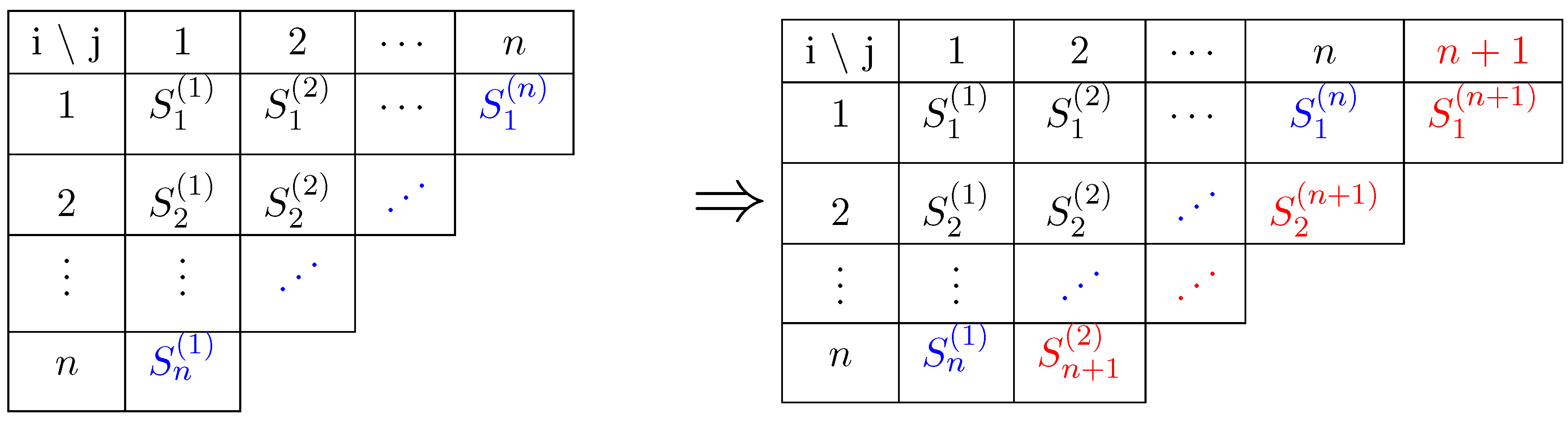
at an intermediate step i, the number of exposures is $N_i$ and the number of losses obtained at this step is given by:

$$S_{N_i}^{\left(i\right)}:=\sum _{j=1}^{N_i}{X}_{j+A_{i-1}}\stackrel{d}{=}\sum _{j=1}^{N_i}{X}_j=:S_{N_i},$$

(3)

(the equality in distribution is discussed and proved in Appendix A) setting $S_{·}:={\sum }_{j=1}^{·}{X}_j$, and is, conditionally on $N_i$, a binomial rv $\left(S_{N_i}^{\left(i\right)}|N_i=n_i\right)\sim \mathcal{B}(n_i,p)$, which we denote as

$$\left(S_{N_i}^{\left(i\right)}|N_i\right)\sim \mathcal{B}(N_i,p).$$

Recall (see e.g., Mikosch 2004) that, by independence of $N_i$ and X, we have

$$\mathbb{E}\left[S_{N_i}^{\left(i\right)}\right]=\mathbb{E}\left(X\right)\mathbb{E}\left(N_i\right)=p\mathbb{E}\left(N_i\right)$$

(4)

and

$$\mathrm{var}\left(S_{N_i}^{\left(i\right)}\right)=\mathbb{E}\left(N_i\right)\mathrm{var}\left(X\right)+\mathrm{var}\left(N_i\right){\left(\mathbb{E}\left(X\right)\right)}^2=p(1-p)\mathbb{E}\left(N_i\right)+p^2\mathrm{var}\left(N_i\right)$$

(5)

(ii)

up to an intermediate step i, the total number of exposures is $A_i$ and the total number of losses is given by

$$S^{\left(i\right)}:=\sum _{j=1}^i{S}_{N_j}^{\left(j\right)}=\sum _{j=1}^i\sum _{k=1}^{N_j}{X}_{k+A_{j-1}}=\sum _{k=1}^{A_i}{X}_k=S_{A_i}$$

and is, conditionally on $(N_j,1\le j\le i)$, a binomial rv:

$$\left(S_{A_i}|(N_j,1\le j\le i)\right)\sim \mathcal{B}\left(A_i,p\right).$$

Here, we have ${\displaystyle \mathbb{E}\left[S_{A_i}\right]=\mathbb{E}\left(X\right)\sum _{k=1}^i\mathbb{E}\left(N_k\right)=p\sum _{k=1}^i\mathbb{E}\left(N_k\right)}$ and

$$\mathrm{var}\left(S_{A_i}\right)=\mathrm{var}\left(X\right)\sum _{k=1}^i\mathbb{E}\left(N_k\right)+{\left(\mathbb{E}\left(X\right)\right)}^2\mathrm{var}\left(A_i\right)=p(1-p)\sum _{k=1}^i\mathbb{E}\left(N_k\right)+p^2\mathrm{var}\left(A_i\right).$$

(iii)

at the end of the multi-steps process under condition (H), the total number of exposures is n and the total number of losses is, as in the one-step case

$$S_n=\sum _{i=1}^n{X}_i\sim \mathcal{B}(n,p)=U\left(n\right).$$

This is what is called the ultimate loss, once the process is completed.

Summarizing the notation, $S_{N_i}^{\left(i\right)}$ is the rv of the losses at the intermediate step i, $S_{A_i}$ is the rv of the losses up to the intermediate step i and $S_n$ is the rv of the ultimate losses $U\left(n\right)$.

For $1\le i\le n$, ${\mathcal{N}}_i$ the $\sigma$-algebra (as usual, ${\mathcal{N}}_0$ or ${\mathcal{F}}_0$ denote the trivial $\sigma$-algebra $\{\varnothing ,\mathsf{\Omega }\}$) generated by the sequence of the rvs $(N_j,1\le j\le i)$

$${\mathcal{N}}_i=\sigma \left\{N_j,1\le j\le i\right\}$$

(6)

and let ${\mathcal{F}}_i$ denote the $\sigma$-algebra generated by the sequence of the rvs $(N_j,1\le j\le i)$ and the corresponding losses $(X_j,1\le j\le N_1+\dots +N_i)$:

$${\mathcal{F}}_i=\sigma \left\{\left(N_j,1\le j\le i\right),\left(X_j,1\le j\le \sum _{k=1}^i{N}_k\right)\right\}.$$

(7)

Note that $\forall 1\le i\le n$, ${\mathcal{N}}_i\subset {\mathcal{F}}_i$.

The process described here would generate a loss triangle following a Bornhutter–Ferguson (Bornhuetter and Ferguson 1972) type of dynamic, which is essentially linear in the error propagation as in our example, and would lead this way to the ultimate. This type of dynamic is typical of certain lines of business mentioned in the introduction and often used by reserving actuaries to estimate the ultimate loss. Such loss triangle will be generated assuming independency across different underwriting years. This assumption, together with the independency between development periods already mentioned in the introduction of Section 2, are simplifications which allow to calculate explicitly the quantities of interest (below) and are anyway two of the assumptions behind the Merz–Wüthrich methodology, which is the standard actuarial methodology object of our study.

2.2. Random Variables of Interest

Now, let us introduce some variables of interest, namely:

• the ultimate loss $U\left(n\right)$, which is $S_n$,
• the expected ultimate loss, given the information up to the step i (for $1\le i\le n)$:

  $$U\left(i\right):=\mathbb{E}\left[U\left(n\right)|{\mathcal{F}}_i\right]=\sum _{j=1}^i{S}_{N_j}^{\left(j\right)}+\mathbb{E}\left[\sum _{j=i+1}^n{S}_{N_j}^{\left(j\right)}|{\mathcal{N}}_i\right],$$

  (8)

  the $X_i$ s being independent of the $N_i$s. Note that we can also define

  $$U\left(0\right):=\mathbb{E}\left[U\left(n\right)|{\mathcal{F}}_0\right]=\mathbb{E}\left[U\left(n\right)\right]=\mathbb{E}\left[S_n\right]=np,$$

  (9)

  which corresponds to the expected loss at ultimate. Note that Equation (8) defines a martingale. Note also that it is a real number (although the rvs are integer valued).
• the variation $D\left(i\right)$ of the expected ultimate loss between two successive steps defines exactly the one year change, when choosing yearly steps:

  $$D\left(i\right)=U\left(i\right)-U(i-1).$$

  (10)
  Here $D\left(i\right)$ is also a real rv. When $i=1$, the $D\left(1\right)$ is closely related to the solvency capital required as defined in the Solvency II framework, which reflects the risk of changes in the technical provision in one year. The difference lies in that $D\left(1\right)$ does not take into account the risk margin change. However, this is of minor importance in the SCR estimation because the risk margin change is of a smaller order of magnitude. Indeed, in practice, it is commonly accepted that the risk margin, which represents the risk loading for the market value of the liability, is approximately constant from one year to the other. We note here that the $D\left(i\right)$s are the innovation of the martingale defined in Equation (8).

For simplicity, all the quantities of interest are considered undiscounted in our paper. The discounting would anyway not invalidate our findings, but only make the calculations more complex.

Note that, as in (ii), we can express the expected ultimate loss using the conditional expectations, as

$$U\left(n\right)=U\left(0\right)+\sum _{i=1}^{n}D\left(i\right).$$

(11)

The goal of this study is to understand better the behavior of $D\left(i\right)$. This means looking for the distribution of $U\left(i\right)$.

Using (8) and (10), and the properties of the conditional expectation, we can write, after straightforward computations,

$$D\left(i\right)=S_{N_i}^{\left(i\right)}+\mathbb{E}\left[\sum _{j=i+1}^n{S}_{N_j}^{\left(j\right)}|{\mathcal{N}}_i\right]-\mathbb{E}\left[\sum _{j=i}^n{S}_{N_j}^{\left(j\right)}|{\mathcal{N}}_{i-1}\right]$$

(12)

so that

$$\mathbb{E}\left[\sum _{j=i+1}^n{S}_{N_j}^{\left(j\right)}|{\mathcal{N}}_i\right]=\mathbb{E}\left[\sum _{j=A_i+1}^{A_i+(n-A_i)}{X}_j|{\mathcal{N}}_i\right]=(n-A_i)\mathbb{E}\left[X\right].$$

Applying (12) provides

$$D\left(i\right)=S_{N_i}^{\left(i\right)}+p\left(n-A_i\right)-p\left(n-A_{i-1}\right)=S_{N_i}^{\left(i\right)}-N_{i}p.$$

(13)

We can see from (13) that $D\left(i\right)$ depends on $N_i$ but also on the past information via $A_{i-1}$. We can then write the probability distribution of $D\left(i\right)$ conditional on this information:

$$\begin{array}{ccc}\mathbb{P}\left(D\left(i\right)=x|A_{i-1}=a_{i-1}\right)& =& \mathbb{P}\left(S_{N_i}^{\left(i\right)}-N_{i}p=x|A_{i-1}=a_{i-1}\right)\hfill \\ & =& \sum _{j=0}^{n-a_{i-1}}\mathbb{P}\left(S_j^{\left(i\right)}-jp=x|A_{i-1}=a_{i-1},N_i=j\right)\hfill \\ & & ·\mathbb{P}\left(N_i=j|A_{i-1}=a_{i-1}\right)\hfill \\ & =& \sum _{j=0}^{n-a_{i-1}}\mathbb{P}\left(S_j-jp=x\right)·\mathbb{P}\left(N_i=j|A_{i-1}=a_{i-1}\right)\hfill \end{array}$$

(14)

using the independence between the $X_i$s and the $N_j$s in the equation before the last, and (3) in the last one.

Let us now choose a probability distribution for the $N_i$s. This choice is arbitrary. We could, for instance, use various distributions typical for modelling frequency or emergence of claims in actuarial modelling, like the Poisson distribution. For simplicity, we will pick first the case of a uniform distribution conditionally to $\mathcal{N}$ so that, for $2\le i\le n-1$, we have

$$\mathbb{P}\left[N_i=n_i|(N_j=n_j,1\le j\le i-1)\right]=\frac{1}{1+n-{\sum }_{j=1}^{i-1}{n}_j}.$$

We remind the reader that $n={\sum }_{i=1}^n{N}_i$. Strictly speaking, we do not even need to have $N_1,\dots ,N_{i-1}$ explicitly. Only their sum matters so that

$$\mathbb{P}\left[N_i=n_i|A_{i-1}=a_{i-1}\right]=\frac{1}{1+n-a_{i-1}}.$$

(15)

We can now proceed to compute the expectation of $N_i$.

Proposition 1.

The expectation of $N_i$ as a function of i is equal to:

$$\mathbb{E}\left(N_i\right)=\frac{n}{2^i}\mathrm{for}i=1,\cdots ,n-1.$$

(16)

Proof of Proposition 1.

Using the property of the conditional expectation, then that $N_1$ is uniformly distributed, and finally the linearity of the expectation, we obtain:

$$\mathbb{E}\left(N_i\right)=\mathbb{E}\left(\mathbb{E}\left(N_i\right|{\mathcal{F}}_{i-1})\right)=\mathbb{E}\left(\frac{n-{\sum }_{j=1}^{i-1}{N}_j}{2}\right)=\frac{1}{2}n-\frac{1}{2}\sum _{j=1}^{i-1}\mathbb{E}\left(N_j\right).$$

(17)

Let us prove the proposition by induction. For $i=1$, by uniformity of the distribution of the rv N, we have:

$$\mathbb{E}\left(N_1\right)=\sum _{n_1=0}^n{n}_1\mathbb{P}[N_1=n_1]=\frac{n}{2}.$$

Suppose (16) is true for any $i\le j-1$ and let us prove it for $i=j$. This is straightforward using (17). Thus, the result ${\displaystyle \mathbb{E}\left(N_j\right)=\frac{1}{2}n\left(1-\sum _{i=1}^{j-1}\frac{1}{2^i}\right)=\frac{n}{2^j}}$. ☐

The last step has actually the same expectation as the previous one since it is the complementary and is completely conditioned by the sum of the previous steps

$$\mathbb{E}\left(N_n\right)=\mathbb{E}\left(n-\sum _{j=1}^{n-1}{N}_j\right)=n-\sum _{j=1}^{n-1}\mathbb{E}\left(N_j\right)=n-\sum _{j=1}^{n-1}\frac{n}{2^j}=\frac{n}{2^{n-1}}.$$

(18)

We have thus fully characterized the expectation of the number of exposures at each step. (In the Appendix B one can find the distribution of the $N_i$ and also of the $D\left(i\right)$.)

3. Analytical Expressions of Quantities to Be Studied

3.1. Incremental Pattern and Capital

Another quantity of interest is the incremental pattern ${\gamma }_i$ of the expected value of the losses. It can be written, using (4) and (9), as:

$${\gamma }_i:=\frac{\mathbb{E}\left(S_{N_i}^{\left(i\right)}\right)}{\mathbb{E}\left(U\right(n\left)\right)}=\frac{1}{2^i},\mathrm{for}i=1,\cdots ,n-1.$$

(19)

For computing the RM, we need to compute the capital requirement (SCR) at each step, using the risk measures ${\mathrm{VaR}}_{99.5\%}$ and ${\mathrm{TVaR}}_{99\%}$, which we will simply call $\rho$. We define the capital requirement $C_i$ at step i as

$$C_i\equiv \mathbb{E}\left(\rho \left(D\left(i\right)\right|{\mathcal{F}}_{i-1})\right).$$

(20)

Once we have this quantity, we can then write the RM, $R_n$, as a function of the number of steps n, as:

$$R_n=\eta \sum _{i=1}^n{C}_i,$$

(21)

where $\eta$ designates the cost of capital.

3.2. Moments of $D\left(i\right)$

The properties we present here are specific to our choice of process, but they can be easily generalized in the framework of martingale assumptions. Let us compute the first two conditional moments of the vector $\mathbf{D}=\left(D\right(1),\dots ,D(n\left)\right)$ given $\mathcal{F}$.

Proposition 2.

Let $0\le i\le n-1$. For k such that $i<k\le n$, we have

(i) 

$$\mathbb{E}\left[D\left(k\right)\right|{\mathcal{F}}_i]=0,$$

(22)

(ii) 

$$\mathrm{var}\left(D\left(k\right)\right|{\mathcal{F}}_i)=\left\{\begin{array}{cc}\frac{\left(n-A_i\right)p(1-p)}{{\displaystyle 2^{k-i}}}\hfill & ifk\ne n,\hfill \\ \frac{\left(n-A_i\right)p(1-p)}{{\displaystyle 2^{n-i-1}}}\hfill & ifk=n,\hfill \end{array}\right.$$

(23)

(iii) 

For $k=i+1$,

$$\mathrm{Cov}\left(\mathbf{D}(i+1)\right|{\mathcal{F}}_i)=p(1-p)\left(n-A_i\right)·\left(\begin{array}{cccc}{2}^{-1}& 0& \cdots & 0\\ 0& 2^{-2}& \ddots & ⋮\\ ⋮& \ddots & \ddots \\ 2^{1+i-n}& 0\\ 0& \cdots & 0& 2^{1+i-n}\end{array}\right),$$

(24)

where $\mathbf{D}(i+1):=\left(D\right(i+1),\dots ,D(n\left)\right)$.

Corollary 1.

From which, we can deduce the following two expressions as corollary:

(a) 

As a consequence of the Proposition 2, the moments of $\mathbf{D}$ are given by

$$\mathbb{E}\left(\mathbf{D}\right)=0\mathrm{and}\mathrm{Cov}\left(\mathbf{D}\right)=np(1-p)·\left(\begin{array}{cccc}{2}^{-1}& 0& \cdots & 0\\ 0& 2^{-2}& \ddots & ⋮\\ ⋮& \ddots & \ddots \\ 2^{1-n}& 0\\ 0& \cdots & 0& 2^{1-n}\end{array}\right).$$

(25)

(b) 

The conditional variance of the ultimate is

$$\mathrm{var}\left(U\left(n\right)\right|{\mathcal{F}}_i)=\left(n-A_i\right)p(1-p).$$

Proof of Proposition 2.

(i) Using the definitions (8) and (10) and the tower property (with $k>i$) produces

$$\mathbb{E}\left[D\left(k\right)\right|{\mathcal{F}}_i]=\mathbb{E}\left(\mathbb{E}\left[U\left(n\right)\right|{\mathcal{F}}_k]|{\mathcal{F}}_i\right)-\mathbb{E}\left(\mathbb{E}\left[U\left(n\right)\right|{\mathcal{F}}_{k-1}]|{\mathcal{F}}_i\right)=\mathbb{E}\left[U\left(n\right)\right|{\mathcal{F}}_i]-\mathbb{E}\left[U\left(n\right)\right|{\mathcal{F}}_i]=0.$$

(ii) The conditional variance of $D\left(i\right)$ can be obtained in the following way: again, take $k\in \{i+1,\dots ,n\}$, and recall the general property of conditional variance, for two random variables X and Y, $\mathrm{var}\left(X\right)=\mathbb{E}\left(\mathrm{var}\right(X\left|Y\right))+\mathrm{var}(\mathbb{E}\left(X\right|Y\left)\right)$. By using this result on $\mathrm{var}\left(D\left(k\right)\right|{\mathcal{F}}_i)$, we obtain

$$\mathrm{var}\left(D\left(k\right)\right|{\mathcal{F}}_i)=\mathbb{E}\left(\mathrm{var}\left(D\left(k\right)\right|N_k)\right|{\mathcal{F}}_i)+\mathrm{var}\left(\mathbb{E}\left(D\left(k\right)\right|N_k)\right|{\mathcal{F}}_i).$$

(26)

We now use Equation (13) on both terms of the right side of the last equation. Since $S_{N_k}^{\left(k\right)}\sim \mathcal{B}(N_k,p)$,

$$\mathbb{E}\left(D\left(k\right)\right|N_k)=\mathbb{E}\left(S_{N_k}^{\left(k\right)}-N_{k}p|N_k\right)=\underset{=N_{k}p}{\underbrace{\mathbb{E}\left(S_{N_k}^{\left(k\right)}|N_k\right)}}-N_{k}p=0,$$

which sets the second term of Equation (26) to 0. Let us calculate the first term.

$$\begin{array}{ccc}\hfill \mathbb{E}\left(\mathrm{var}\left(D\left(k\right)|N_k\right)|{\mathcal{F}}_i\right)& =& \mathbb{E}\left(\mathrm{var}\left(S_{N_k}^{\left(k\right)}-N_{k}p|N_k\right)|{\mathcal{F}}_i\right)\hfill \\ & =& \mathbb{E}\left(\mathrm{var}\left(S_{N_k}^{\left(k\right)}|N_k\right)|{\mathcal{F}}_i\right)\hfill \\ & =& \mathbb{E}\left(N_{k}p(1-p)\right|{\mathcal{F}}_i)\hfill \\ & =& p(1-p)\mathbb{E}\left(N_k\right|{\mathcal{F}}_i).\hfill \end{array}$$

We now consider the following argument: Assuming ${\mathcal{F}}_i$ known, is equivalent in terms of rvs to starting a new process with $n-i$ steps and $n-A_i$ rvs. A generalization of Equations (16) and (18) therefore gives

$$\mathbb{E}\left(N_k\right|{\mathcal{F}}_i)=\frac{n-A_i}{2^{k-i}},\mathrm{if}k\in \{i+1,\dots ,n-1\}$$

and

$$\mathbb{E}\left(N_n\right|{\mathcal{F}}_i)=\mathbb{E}\left(N_{n-1}\right|{\mathcal{F}}_i)=\frac{n-A_i}{2^{n-i-1}}.$$

It follows then that

$$\mathrm{var}\left(D\left(k\right)\right|{\mathcal{F}}_i)=\frac{\left(n-A_i\right)p(1-p)}{2^{k-i}}\mathrm{if}k\ne n$$

and that

$$\mathrm{var}\left(D\left(n\right)\right|{\mathcal{F}}_i)=\frac{\left(n-A_i\right)p(1-p)}{2^{n-i-1}}.$$

We also notice that, since $N_n=n-A_{n-1}$ is ${\mathcal{F}}_{n-1}-$measurable,

$$\mathrm{var}\left(D\left(n\right)\right|{\mathcal{F}}_{n-1})=\mathrm{var}\left(S_{N_n}^{\left(n\right)}|{\mathcal{F}}_{n-1}\right)=N_{n}p(1-p).$$

This finishes the calculation of the conditional variance.

(iii) Only calculation of the conditional covariance remains. Let $i\in \{0,1,\dots ,n-2\}$ and $j,k\in \{i+1,\dots ,n\},\mathrm{with}j<k$. Since $\mathbb{E}\left(D_j\right|{\mathcal{F}}_i)=0$,

$$\begin{array}{ccc}\hfill \mathrm{Cov}(D\left(j\right),D\left(k\right)|{\mathcal{F}}_i)& =& \mathbb{E}\left(D\left(j\right)D\left(k\right)\right|{\mathcal{F}}_i)\hfill \\ & =& \mathbb{E}\left(\mathbb{E}\left(D\left(j\right)D\left(k\right)\right|{\mathcal{F}}_j)\right|{\mathcal{F}}_i)\hfill \\ & =& \mathbb{E}(D\left(j\right)\underset{=0}{\underbrace{\mathbb{E}\left(D\left(k\right)\right|{\mathcal{F}}_j)}}|{\mathcal{F}}_i)=0.\hfill \end{array}$$

This finishes the characterization of the second moment of $\mathbf{D}\left(i\right)$. Indeed, we have shown that $\forall i\in \{0,1,\dots ,n-1\}$,

$$\mathbb{E}\left(\mathbf{D}(i+1)\right|{\mathcal{F}}_i)=0$$

and

$$\mathrm{Cov}\left(\mathbf{D}(i+1)\right|{\mathcal{F}}_i)=p(1-p)\left(n-A_i\right)·\left(\begin{array}{cccc}{2}^{-1}& 0& \cdots & 0\\ 0& 2^{-2}& \ddots & ⋮\\ ⋮& \ddots & \ddots \\ 2^{1+i-n}& 0\\ 0& \cdots & 0& 2^{1+i-n}\end{array}\right).$$

(27)

 ☐

Proof of Corollary 1.

Since the particular case $i=1$ corresponds to the unconditional moments of $\mathbf{D}$, we have:

$$\mathbb{E}\left(\mathbf{D}\right)=\mathbb{E}\left(\mathbf{D}\right|{\mathcal{F}}_0)\mathrm{and}\mathrm{Cov}\left(\mathbf{D}\right)=\mathrm{Cov}\left(\mathbf{D}\right|{\mathcal{F}}_0).$$

(a)

Thus, the unconditional moments of D are given by

$$\mathbb{E}\left(\mathbf{D}\right)=0\mathrm{and}\mathrm{Cov}\left(\mathbf{D}\right)=np(1-p)·\left(\begin{array}{cccc}{2}^{-1}& 0& \cdots & 0\\ 0& 2^{-2}& \ddots & ⋮\\ ⋮& \ddots & \ddots \\ 2^{1-n}& 0\\ 0& \cdots & 0& 2^{1-n}\end{array}\right),$$

(28)

(b)

As an immediate consequence of Equation (24), one can write the conditional variance of the ultimate as

$$\begin{array}{cc}\hfill \mathrm{var}\left(U\left(n\right)\right|{\mathcal{F}}_i)& =\mathrm{var}\left(U\left(0\right)+\sum _{j=1}^{i}D\left(j\right)+\sum _{j=i+1}^{n}D\left(j\right)|{\mathcal{F}}_i\right)\hfill \\ & =\sum _{j=i+1}^n\mathrm{var}\left(D\left(j\right)|{\mathcal{F}}_i\right)=\left(n-A_i\right)p(1-p).\hfill \end{array}$$

(This formula can also be derived directly, arguing that $U\left(n\right)|{\mathcal{F}}_i\sim \mathcal{B}\left(n-{\sum }_{j=1}^i{N}_j,p\right)$.) ☐

3.3. Completion Time

Our process is defined on a finite time scale of n-steps. However, the process will, most of the time, finish much before the n-th step (the ultimate time). It is therefore of interest to know how fast the process reaches the maximum exposures allowed. This is also very important for computational reasons. Indeed, when simulating from the process, one can stop the simulation procedure earlier than the ultimate time thus sparing large amounts of calculations. In order to answer this question, we first consider a type of process that differs slightly from ours in the sense that it has an infinite time range (infinite steps), but is still only allowed a finite number of exposures, n. For an infinite time process with n rvs, let us denote by

$$T_n=inf\left\{t:\sum _{k=1}^t{N}_k=n\right\}$$

the completion time given by the step at which the last exposure is realized. Before trying to approximate a finite process with an infinite process, we need to show that the infinite process finishes with probability 1.

Proposition 3.

The probability of the completion time at infinity is 0:

$$P(T_n=\infty )=0.$$

(29)

Proof of Proposition 3.

For $n=1$, we can argue that

$$\begin{array}{cc}\hfill \mathbb{P}(T_1=\infty )& =\underset{=0}{\underbrace{\mathbb{P}(T_1=\infty |N_1=1)}}\underset{=\frac{1}{2}}{\underbrace{\mathbb{P}(N_1=1)}}+\underset{=\mathbb{P}(T_1=\infty )}{\underbrace{\mathbb{P}(T_1=\infty |N_1=0)}}\underset{=\frac{1}{2}}{\underbrace{\mathbb{P}(N_1=0)}}\hfill \\ & =\frac{1}{2}\mathbb{P}(T_1=\infty ),\hfill \end{array}$$

which implies that $\mathbb{P}(T_1=\infty )=0$. Note that $\mathbb{P}(T_1=\infty |N_1=0)=\mathbb{P}(T_1=\infty )$ is justified by the fact that, since the process is infinite, assuming $N_1=k$ is equivalent to starting a new infinite process with $n-k$ rvs. This argument is used here with $k=0$ but is explained with general k because we will use it further for other values of k. For $n>1$, we can do very similar calculations by induction. Assume that $\mathbb{P}(T_i=\infty )=0$, $\forall i\in \{1,\dots ,n-1\}$. Then,

$$\begin{array}{cc}\hfill \mathbb{P}(T_n=\infty )& =\underset{=\mathbb{P}(T_n=\infty )}{\underbrace{\mathbb{P}(T_n=\infty |N_1=0)}}\underset{=\frac{1}{n+1}}{\underbrace{\mathbb{P}(N_1=0)}}+\sum _{k=1}^n\underset{=\mathbb{P}(T_{n-k}=\infty )}{\underbrace{\mathbb{P}(T_n=\infty |N_1=k)}}\underset{=\frac{1}{n+1}}{\underbrace{\mathbb{P}(N_1=k)}}\hfill \\ & =\frac{1}{n+1}\mathbb{P}(T_n=\infty )+\frac{1}{n+1}\sum _{k=1}^n\underset{=0\mathrm{by}\mathrm{ind}.\mathrm{hyp}.}{\underbrace{\mathbb{P}(T_{n-k}=\infty )}}\hfill \\ & =\frac{1}{n+1}\mathbb{P}(T_n=\infty ),\hfill \end{array}$$

which again proves that $P(T_n=\infty )=0$. ☐

Since the process finishes with probability 1 and the probability of an infinite process with n rvs finishing after time n is very small for n large enough, the approximation is very reasonable.

We would like to find a formula for $\mathbb{E}\left(T_n\right)$. By conditioning on the first step, we obtain

$$\mathbb{E}\left(T_n\right)=\mathbb{E}\left(\mathbb{E}\left(T_n\right|{\mathcal{F}}_1)\right)=\sum _{k=0}^n\mathbb{E}\left(T_n\right|N_1=k)\mathbb{P}(N_1=k).$$

Again, assuming $N_1=k$ is equivalent to starting a new process with $n-k$ rvs. Therefore, $\mathbb{E}\left(T_n\right|N_1=k)=1+\mathbb{E}\left(T_{n-k}\right)$, where the 1 takes into account the first step. As $\mathbb{E}\left(T_n\right)$ only depends on n, let us denote it by $\mathbb{E}\left(T_n\right)=f\left(n\right)$. We can then write the following iterative formula

$$f\left(n\right)=\frac{1}{n+1}\sum _{k=0}^n(1+f(n-k))=1+\frac{f\left(0\right)+\dots +f\left(n\right)}{n+1}.$$

Solving for $f\left(n\right)$ and realising that $f\left(0\right)=0$, we obtain

$$f\left(n\right)=1+\frac{1+f\left(1\right)+\dots +f(n-1)}{n},$$

which gives by iteration, for $n\ge 2$:

$$f\left(n\right)=\frac{1}{n}+f(n-1).$$

(30)

Note that

$$f\left(1\right)=\mathbb{E}\left(T_1\right)=\sum _{j=1}^{\infty }j\mathbb{P}(T_1=j)=\sum _{j=1}^{\infty }j\frac{1}{2}\frac{1}{2^{j-1}}=2.$$

Hence, by iterating Equation (30), we obtain the formula

$$f\left(n\right)=f\left(1\right)+\sum _{j=2}^n\frac{1}{j}=1+\sum _{j=1}^n\frac{1}{j}.$$

(31)

We have now an expression that gives the average completion time of an infinite process as 1 plus the truncated harmonic series, which can itself be approximated by

$$f\left(n\right)=1+\sum _{j=1}^n\frac{1}{j}=1+\gamma +ln\left(n\right)+\mathcal{O}\left(n^{-1}\right)\approx ln\left(n\right)+1.57,$$

(32)

where $\gamma \approx 0.5772$ is the Euler constant. If n is large enough, we therefore have a simple way to estimate approximately how many steps the process will last on average.

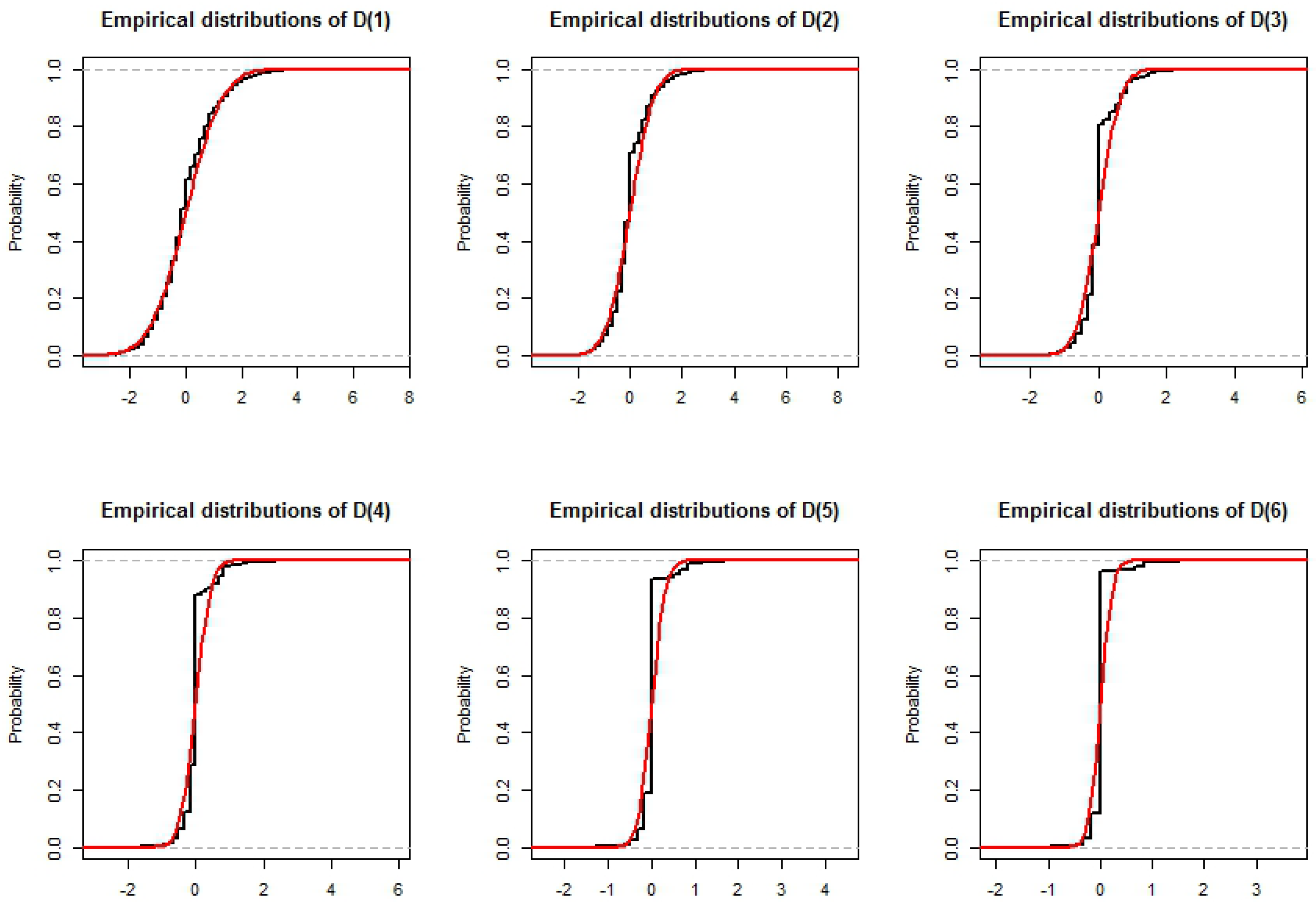
3.4. Distribution of the $D\left(i\right)$

In Section 3.2, we studied analytically the two first moments of the $D\left(i\right)$. Here, we simulate 200,000 times the process of size $n=15$ to estimate the empirical distribution of the $D\left(i\right)$. We also compute the normal distribution with same mean and variance to compare the distributions. The results are displayed in Figure 1. Let us recall Equation (13), which states $D\left(i\right)=S_{N_i}^{\left(i\right)}-N_{i}p$. Conditional on $N_i$, this random variable has centered binomial distribution (i.e., binomial distribution minus its average). The Central Limit Theorem applies to binomial rv X with parameters n, p. Thus, the distribution, f, of a sum of n independent Bernoulli rvs with parameter p will converge to a Gaussian distribution: ${\displaystyle f\left(X\right)\approx \mathcal{N}\left(np,np(1-p)\right)}$, for n large enough. Assume that F is a discrete mixture of normal distributions with mean 0, variances ${\sigma }_1^2,\dots ,{\sigma }_N^2$ and weights $p_1,\dots ,p_n$. Then, $\forall x\in \mathbb{R}$,

$$F\left(x\right)=\sum _{i=1}^n{p}_i·\mathbb{P}[W\le x]=\sum _{i=1}^n{p}_i·\mathsf{\Phi }(x/{\sigma }_i),$$

where W is a normal rv $\mathcal{N}(0,{\sigma }_i^2)$. In particular, if for some indices i and j, $1/{\sigma }_i$ and $1/{\sigma }_j$ are close to each other, then $\mathsf{\Phi }(x/{\sigma }_i)$ and $\mathsf{\Phi }(x/{\sigma }_j)$ are also going to be close to each other. In our case, $1/{\sigma }_i={\left(ip(1-p)\right)}^{-1/2}$ and these values are going to be close when i is large enough. If a sufficiently large part of the weight is on large values of i, our mixture of centred binomial distributions is going to be close to a Normal distribution. In other words, $D\left(i\right)$ is going to have a distribution that is close to Normal only if the probability of having a large $N_i$ is high. For $n=15$, as we can see in Figure 1, it is the case. For $i=2$, the approximation is still reasonable despite a mass larger than normal around 0. For $i>2$, the fit is rather good for large and small quantiles but not for the middle part of the distribution. We recall from Equation (16) that expectation of $N_i$ is divided by 2 at every step so that small values of $N_i$ and in particular 0 will have a larger probability. It should be noted that, due to the probability mass of small values of $N_i$, these mixture distributions, even if they are close to a normal distribution, will always have a higher than normal probability density around 0. To verify this intuition empirically, we also simulate 200,000 times the process for sizes $n=50$ and $n=100$. The results do confirm our intuition. Indeed, for $n=50$, the approximation is good for $i=1,2,3$ and starts failing for $i=4$, where $\mathbb{E}\left(N_4\right)=3.125$. For $n=100$, we can of course go one step further, which makes the normal approximation good also for $D\left(4\right)$.

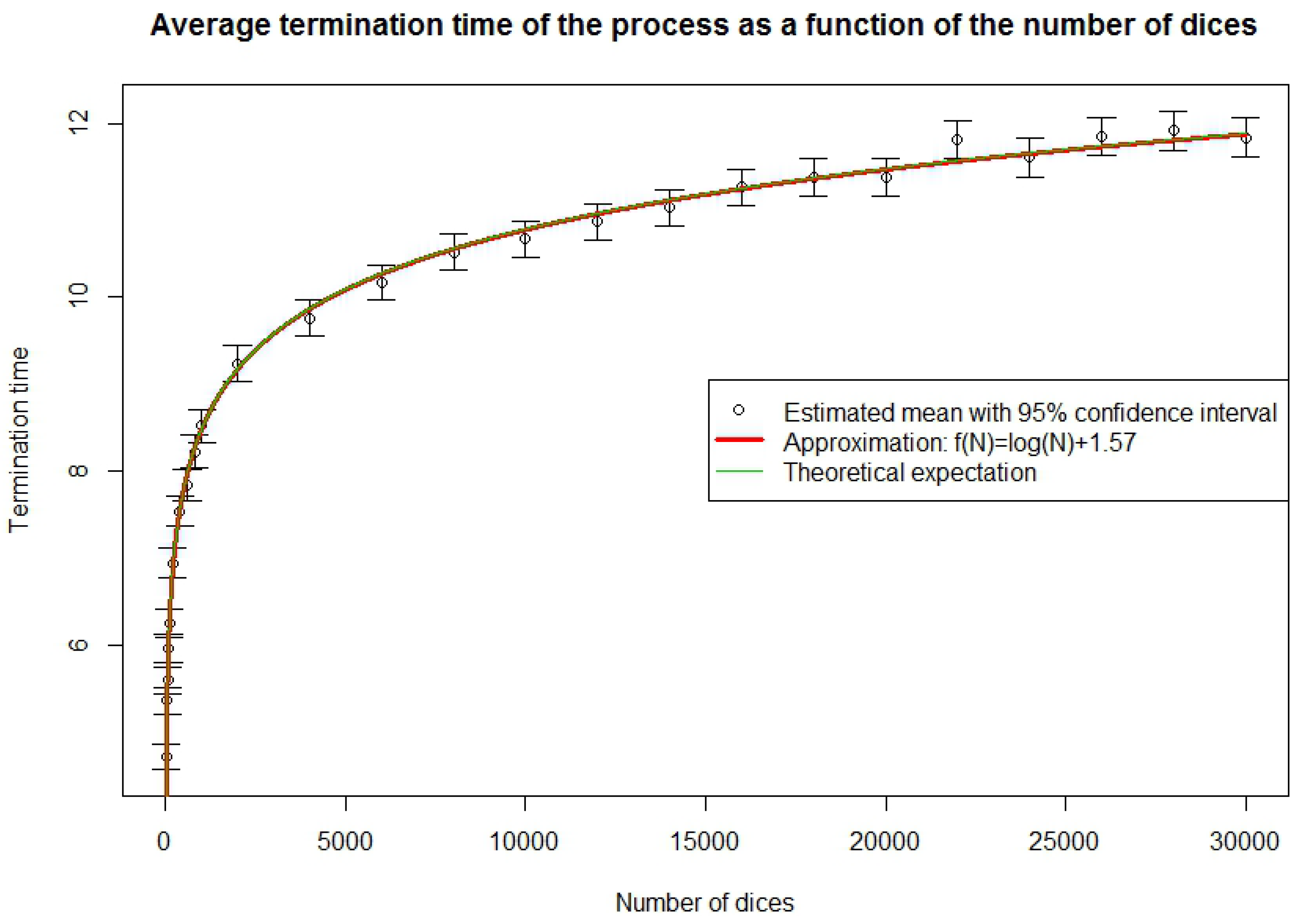
3.5. Simulation of the Completion Time

We have seen, in Section 3.3, Equations (31) and (32), how to approximate the average time until the end of the process. We test this result empirically by simulating 10,000 times the process of size n for $n=20,40,\dots ,100,200,400,\dots ,1000,2000,4000,\dots ,30,000$. For each n, we calculate the average time to complete the total number of exposures and the 95% Gaussian confidence interval given by adding or subtracting 1.96 times the empirical standard deviation of the sample. We also calculate the harmonic series and its approximation by a logarithm. The two approximations are almost identical and fit very well the results. Indeed, in 25 times, the 95% confidence interval misses once, which is what is expected. The approximations should however be expected not to be valid for very short processes because the logarithm approximation is based on convergence and because both the logarithm and harmonic series approximations are based on the approximation of a finite process by an infinite one, which is inaccurate for very short processes. In order to know how long a process must be for the approximation to be valid, we simulate 10,000 times the process of size n for $n=2,\dots ,20$. From the results, displayed in Figure 2, we see that for $n=1,\dots ,6$, the fit is not good. However, from $n\ge 7$ onwards, our approximation is a reasonable and easy way to find the completion time. We shall use this result later when we build loss triangles.

4. Capital Requirements

In this section, we propose a framework to test the accuracy of some of the methods to estimate the one year change. We construct triangles using the model presented in Section 3.4. From these triangles, we estimate the one year change using the classica Merz–Wüthrich method Wüthrich and Merz (2008) and the capital-over-time (COT) method, currently used at SCOR Ferriero (2016). We then compare the results obtained analytically and by simulation based on the specifications of our model to those estimated by the Merz–Wüthrich and with the capital-over-time (COT) method.

4.1. Triangles

Until now, we have only considered the development properties of one process. Actual liability data are generally available in the form of triangles that represent the losses attributed to insurance contracts for each underwriting year after their current numbers of years of development. It is therefore reasonable to compare the results of our model in this framework. We first need to define the notation. Let us consider n representations of the process of size n. We denote their ultimate losses $U_1\left(n\right),\dots ,U_n\left(n\right)$. The ultimate loss of the triangle is then

$$U\left(n\right)=\sum _{i=1}^n{U}_i\left(n\right).$$

We denote by $N_{i,1},\dots ,N_{i,n}$ the number of exposures realized at each step of the ith process and $S_{N_{i,j}}^{\left(j\right)}$ the losses due to $N_{i,j}$. The cumulated losses of row i up to column j are written $S_i^{\left(j\right)}$. We consider the discrete filtration ${\left({\mathcal{F}}_k\right)}_{0\le k\le n}$ given by the information available at each calendar year. Formally,

$${\mathcal{F}}_k=\sigma \left(N_{i,j},S_{N_{i,j}}^{\left(j\right)}:i+j\le n+1+k\right).$$

The individual filtrations of each representation of the process are denoted by

$${\mathcal{F}}_{i,k}=\sigma \left(N_{i,j},S_{N_{i,j}}^{\left(j\right)}:j\le k\right).$$

We denote the jth one-year change of the ith individual process by $D_i\left(j\right)$ and define the one-year changes of the triangle until its completion by

$$\begin{array}{cc}\Delta \left(k\right)& =\mathbb{E}\left(U\left(n\right)\right|{\mathcal{F}}_k)-\mathbb{E}\left(U\left(n\right)\right|{\mathcal{F}}_{k-1})\hfill \\ & =D_{k+1}\left(n\right)+D_{k+2}(n-1)+\dots +D_n(k+1)\hfill \\ & =\sum _{i=k+1}^n{D}_i(n+k+1-i).\hfill \end{array}$$

(33)

Equation (33) simply writes the global one-year change as the sum of the individual one-year changes. Note that, due to linearity of expectation, Equation (33) also implies that the $\Delta \left(i\right)$ have expectation 0 and are uncorrelated. Their variances can be calculated by summing the variances of the individual one-year changes that constitute them.

Similarly to the individual process situation, we define the capital requirement for calendar year i as

$$K_i=\mathbb{E}\left(\rho (\Delta \left(i\right)|{\mathcal{F}}_{i-1})\right),i=1,\dots ,n-1,$$

for some risk measure $\rho$. The risk-margin associated with these capitals is

$$R_n=\eta \sum _{i=1}^{n-1}{K}_i,$$

for the cost of capital $\eta$.

4.2. Methodology and Results’ Comparison

We now describe the methodology used to obtain our risk measure results and to compare them with the Merz–Wüthrich and the COT methods, both briefly explained in Appendix D. For convenience, we use the following notation

$${\tilde{N}}_{i,j}=n-\sum _{k=1}^j{N}_{i,k}$$

for the number of exposures remaining to be realized for row i of the triangle after time j. In particular, $N_{i,j}\sim \mathrm{Unif}\left(\{0,1,\dots ,{\tilde{N}}_{i,j-1}\}\right)$ for $j=1,\dots ,n-1$. In particular, ${\tilde{N}}_{i,j}$ is an ${\mathcal{F}}_{i,j}-$measurable random variable.

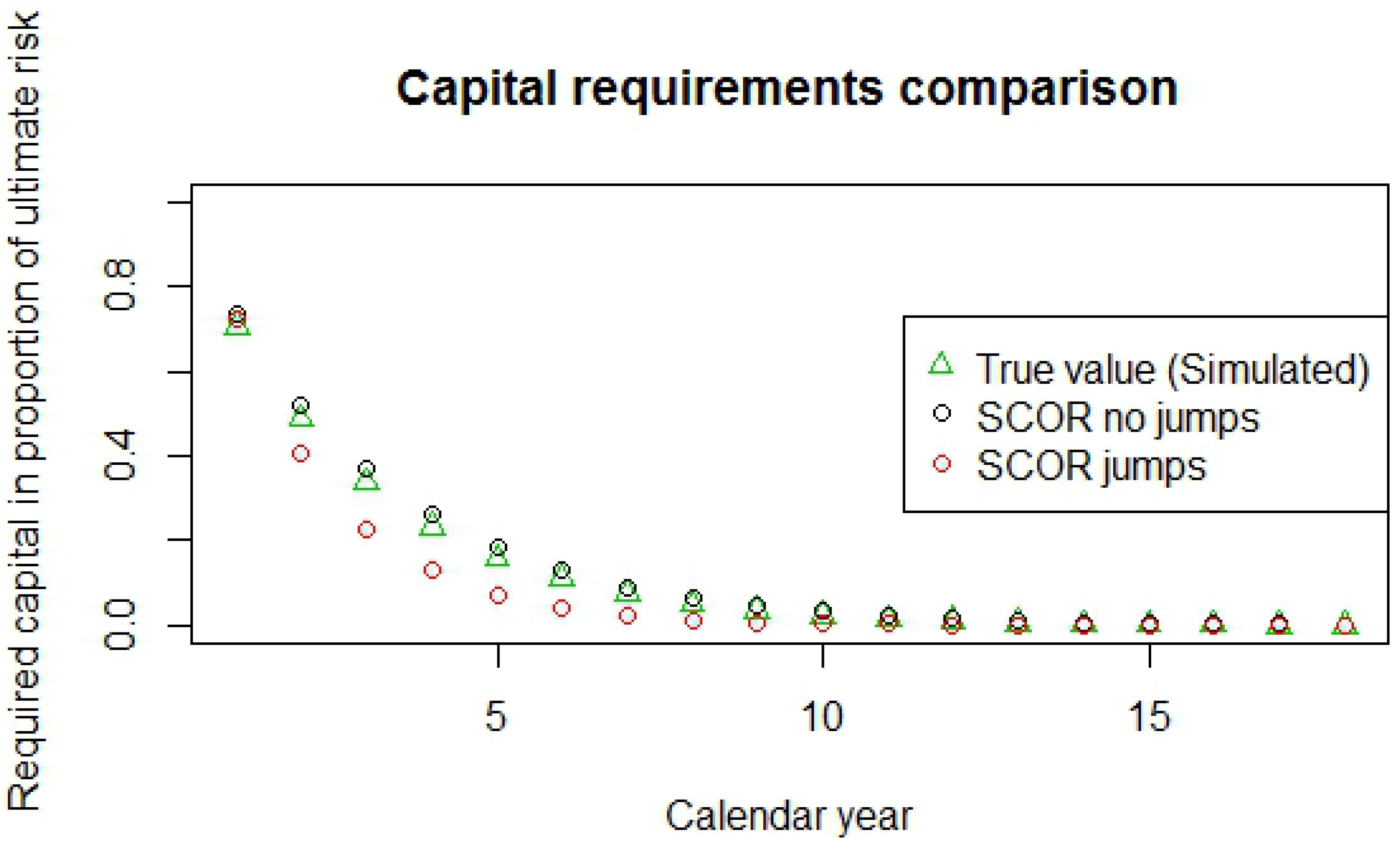
4.2.1. First Year Capital Comparison

A first value of interest is the required capital for the first year

$$K_1={\mathrm{TVaR}}_{\kappa }(\Delta \left(1\right)|{\mathcal{F}}_0).$$

The Merz–Wüthrich method only provides $\mathrm{var}(\Delta \left(1\right)|{\mathcal{F}}_0)$, while the COT method was originally designed for $\mathrm{xTVaR}$ (A4). An assumption concerning the link between $\mathrm{var}$ and $\mathrm{TVaR}$ is therefore to be made. Since $\Delta \left(1\right)|{\mathcal{F}}_0$ follows a mixture of binomial distributions for a generally large number of rvs, its distribution can be approximated relatively well by a normal distribution (this approximation may lead up to 20% underestimation of the risk depending on the number of exposures n). Note that the number of rvs from the binomial is not a uniform variable but a sum of uniform variables, which diminishes the probability of very large or very low values, thus making the normal approximation better than for a simple uniform number of rvs. Normal distribution fixes the relation between $\mathrm{var}$ and $\mathrm{TVaR}$:

$${\mathrm{TVaR}}_{\kappa }\left(\mathcal{N}(\mu ,{\sigma }^2)\right)=\mu +\sigma \underset{\approx 2.665\mathrm{for}99\%}{\underbrace{\frac{\varphi \left({\mathsf{\Phi }}^{-1}\left(\kappa \right)\right)}{1-\kappa }}}.$$

(34)

In our case, $\mu =\mathbb{E}(\Delta \left(1\right)|{\mathcal{F}}_0)=0$ and

$$\begin{array}{cc}{\sigma }^2& =\mathrm{var}(\Delta \left(1\right)|{\mathcal{F}}_0)\hfill \\ & =\mathbb{E}\left(\mathrm{var}(\Delta \left(1\right)|N_{2,n},\dots ,N_{n,2})\right|{\mathcal{F}}_0)+\mathrm{var}\left(\underset{=0}{\underbrace{\mathbb{E}(\Delta \left(1\right)|N_{2,n},\dots ,N_{n,2})}}\right|{\mathcal{F}}_0)\hfill \\ & =\mathbb{E}\left((N_{2,n}+\dots +N_{n,2})p(1-p)\right|{\mathcal{F}}_0)\hfill \\ & =\left({\tilde{N}}_{2,n-1}+\sum _{j=3}^n\frac{{\tilde{N}}_{j,n+1-j}}{2}\right)·p(1-p).\hfill \end{array}$$

(35)

Combining Equations (34) and (35), we can obtain an approximate analytical value for $K_1$,

$$K_1\approx \frac{\varphi \left({\mathsf{\Phi }}^{-1}\left(\kappa \right)\right)}{1-\kappa }·{\left(p(1-p)\right)}^{1/2}·{\left({\tilde{N}}_{2,n-1}+\sum _{j=3}^n\frac{{\tilde{N}}_{j,n+1-j}}{2}\right)}^{1/2}.$$

(36)

The COT method, such as explained in Appendix D, was designed for real insurance data. In particular, parameter b models the dependence between relative loss increments. In the case of our model, the relative loss increments are uncorrelated, which points to the choice of parameter $b=0.5$ instead of the value chosen with mean time to payment. The choice of coefficient $p_b$ is also arbitrary. Indeed, $p_b$ determines the proportion of the risk that is due to the jump part of the process. For our process, there is no “special” type of behaviour that the model could have and that would increase the risk. Therefore, we choose $p_b=0$. In general, the type of data is not known, in particular the dependency between loss increments is not known. Thus, we are also interested in the results given by the COT method applied the standard way. We therefore also compute the COT estimator with $p_b$ chosen according to Formula (A5). In our case, b cannot be chosen like in the formula, as the pattern used in the mean time to payment computation is a paid pattern that we do not have for our model. For the jump case, we choose $b=0.75$ as for a long-tail process. Indeed, the (incurred) pattern of our n-step process corresponds generally to the type of patterns that one can find in long (or possibly medium) tail lines of business. We will refer to the two variations of the method as “COT method with jump part” for the version with standard $p_b$ and $b=0.75$ and “COT method without jump part” for the version with $b=0.5$ and $p_b=0$.

In the case of an n-step Bernoulli model triangle, we notice that the accident-year (incremental) patterns are given by

$${\gamma }_i={\left(\sum _{j=2}^n{\tilde{N}}_{j,n+1-j}\right)}^{-1}·\left(\frac{{\tilde{N}}_{i+1,n-i}}{2^{i-1}}+\sum _{j=i+2}^n\frac{{\tilde{N}}_{j,n+1-j}}{2^i}\right).$$

(37)

The first factor is simply the total number of exposures remaining to be realized, the first row not being counted because it is finished. Since, at each step but the last, half of the current exposures of the process are expected to be realized, the number of exposures remaining for each unfinished is expected to be the number of exposures remaining in the original triangle divided by 2 for each past step that is not the last step. Hence, the expected remaining exposures are

$$\sum _{j=i+2}^n\frac{{\tilde{N}}_{j,n+1-j}}{2^i}$$

for the lines that are not finished after i steps, plus

$$\frac{{\tilde{N}}_{i+1,n-i}}{2^{i-1}}$$

for the line that finishes precisely after i steps. The pattern designates the results of the binomial random variable and not the number of exposures. However, since the rvs (random variable X) are independent and have the same expectation, the numerator and denominator are both multiplied by p leaving the result unchanged.

In particular, with the help of Equation (37) and after few manipulations, we have that

$$\mathrm{var}(\Delta \left(i\right)|{\mathcal{F}}_0)=\mathbb{E}\left(\mathrm{var}(\Delta \left(i\right)|{\mathcal{F}}_{i-1})\right|{\mathcal{F}}_0)+\mathrm{var}(\underset{=0}{\underbrace{\mathbb{E}(\Delta \left(i\right)|{\mathcal{F}}_{i-1})}}|{\mathcal{F}}_0)={\gamma }_i·\mathrm{var}\left(U\left(n\right)\right|{\mathcal{F}}_0).$$

This result uses the property of martingales that the variance of the sum of martingale increments is equal to the sum of variances. An analogous property is false for the $\mathrm{TVaR}$. However, we get for the COT model without jump part, an approximation (see Ferriero 2016)

$${\mathrm{TVaR}}_{\kappa }(\Delta \left(1\right)|{\mathcal{F}}_0)\approx {\gamma }_1^{1/2}·{\mathrm{TVaR}}_{\kappa }\left(U\left(n\right)\right|{\mathcal{F}}_0).$$

Moreover, if we assume that the normal approximation is not an approximation but indeed an exact distribution, it can be shown through straightforward calculations that this expression becomes an exact result for the required capital for the first year (see Ferriero 2016).

The Merz–Wüthrich method is the one posing the most problems. Indeed, the triangles generated with our process are very noisy in the sense that the simulated triangles can quite often have many zeros. The Mack hypotheses, on which the Merz–Wüthrich method is based, are multiplicative in nature and, therefore, very sensitive to zeros. If there is a zero in the first column of a triangle, Mack’s estimation fails to compute the parameters ${\sigma }_1$. There are more robust ways, such as the one developed in Busse et al. (2010), to calculate these estimators. However, all of them (except removing the line) fail if an entire row of the triangle is 0. This happens quite often for n small. If n is large, the problem becomes, as we explain in Section 3.5, that the process terminates on average in time $log\left(n\right)+1.57$, which means that the largest part of the triangle shows no variation at all and gives ${\sigma }_i=0$. In order to eliminate all these problems, we simulate our test triangles with n = 100,000 and work on the truncated top side of the triangle of size $m=\lceil 5+\underset{\approx \mathbb{E}\left(T_n\right)}{\underbrace{log\left(n\right)+1.57}}\rceil =19$, where 5 is a safety margin to insure that the run-off of the process is finished or at least almost finished.

We set $p=0.1\%$, which is a more realistic value given the high number of policies, simulate 500 triangles and, for each of them, calculate the first year capital $K_1$ using the theoretical value, the COT method with and without jumps and the Merz–Wüthrich method. We display, in

Table 1. Statistics for the first year capital on the 500 simulated triangles. The mean first year capital, the standard deviation of the capital around that mean and the mean absolute and relative deviations (MAD/MRAD) from the true value are displayed. The latter are computed using both a standard and the robust Huber M-estimator, Huber (1981). The mean reserves estimated with chain-ladder are 101.87, which are consistent with the reserves calculated with our model, i.e., $n(1-1/2^I)p=100,000(1-2^{19})0.001=100.00$.

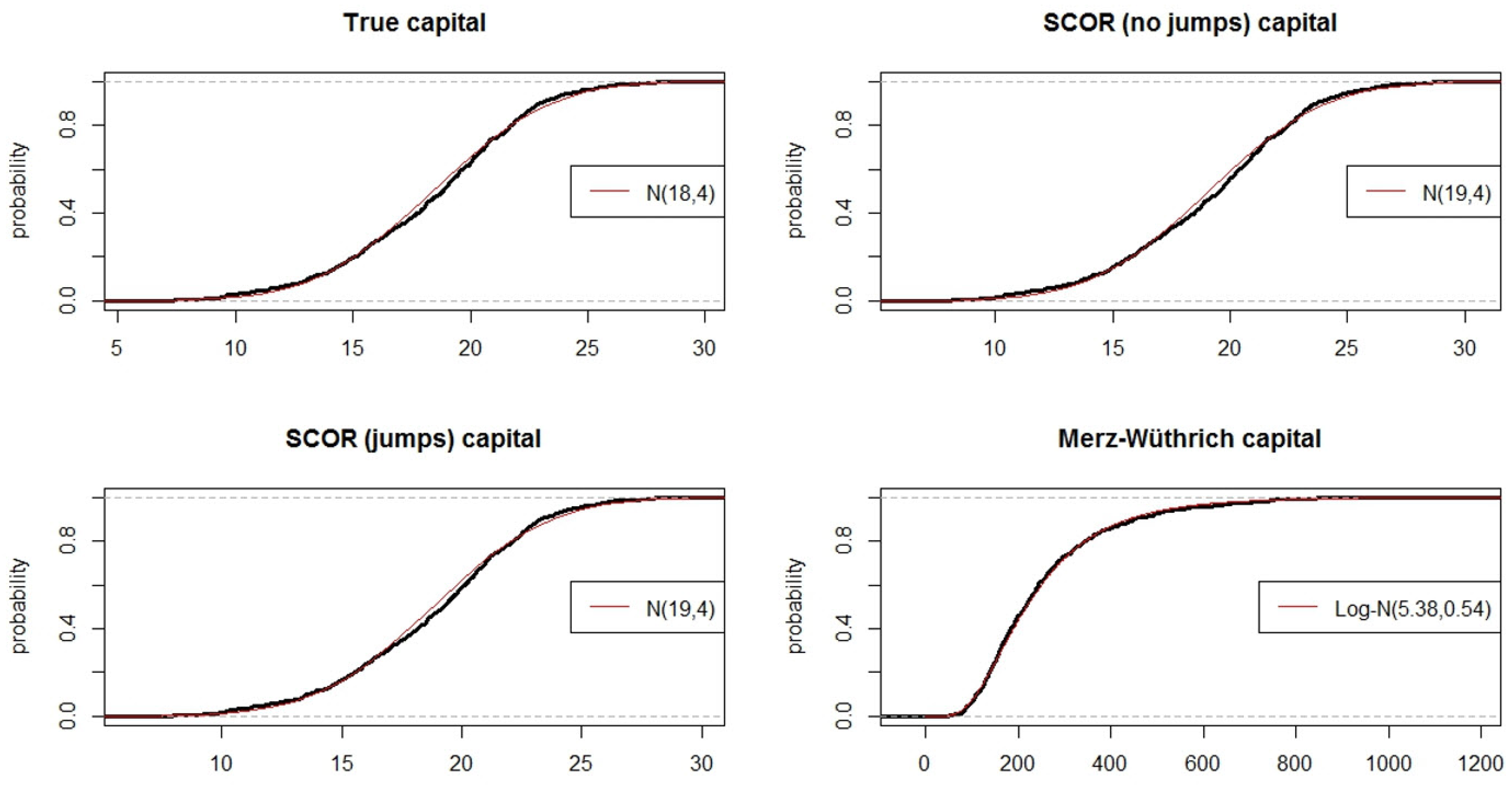
Method	Mean	Std. Dev.	MAD	MRAD	Rob. MAD	Rob. MRAD
Theoretical value	18.37	3.92	0	0%	0	0%
SCOR, without jumps	19.08	3.93	0.71	4.14%	0.71	3.93%
SCOR, with jumps	18.81	3.86	0.43	2.47%	0.44	2.42%
Merz–Wüthrich	252.89	149.6	234.5	1365.6%	213.9	1217.8%

, the mean capital and the standard deviation of the capital around that mean over the 500 triangles. We also calculate the mean absolute deviation (MAD)

$$\mathrm{MAD}=\mathbb{E}\left(|\widehat{X}-X|\right)$$

and mean relative absolute deviation (MRAD)

$$\mathrm{MRAD}=\mathbb{E}\left(\frac{|\widehat{X}-X|}{X}\right)$$

with respect to the theoretical value using standard and robust mean estimation.

Note that, in our example, the relative risk, i.e., the first year capital relative to the reserves volume, is about 18% (the reserves are approximately 100 and the first year capital approximately 18), which is a realistic value. The reserves in our model can be easily computed by the close formula $n(1-1/2^m)p$, as proved in Appendix C. As a point of comparison, using the prescription of the Solvency Standard Formula, we find a stand-alone capital intensity (SCR/Reserves) between 14% to 26% for the P&C reserves. Given the type of risks we are considering here, it is logical that the capital intensity should be at the lower end of the range. By the way, we also see, as expected, that the average claim is much smaller than the maximum claim (100,000) given the fact that the chances that 100,000 independent policies claim at the same time with such a low probability of claims ($p=1‰$) is practically nil.

The results presented in Table 1 are striking. While the COT method gives answers close to the theoretical value with a slight preference, as expected, for the COT without jumps, the Merz–Wüthrich method is way off (1356.6% off the true value), and the true result is not even within one standard deviation away. The coefficient of variation $\sigma /\mu$ for this method is more than 59% while in all the other cases it hovers around 21%. There are many explanations for this. Looking at triangles and analysing the properties of the methods allows us to understand those results. The true risk depends on the number of rvs remaining to be realized. In most cases, only the few last underwriting years are truly important in that matter because the others will be almost fully developed. For Merz–Wüthrich, as most of the volatility of the process will appear on the first step, the most crucial part of the triangle is the last line of the triangle, which is the only process representation at this stage of development. If the latter is large, it influences the Merz–Wüthrich capital in the same direction. Merz–Wüthrich interprets a large value as: “Something happened on that accident year, there is going to be more to pay than expected”. The logic behind our model is different, through the “fixed number of rvs” property, it is: “What has been paid already needs not to be paid anymore”. A large value on the last line of the triangle is therefore likely to indicate that few rvs remain to be realized, which implies smaller remaining risk. This explains negative correlation because the same cause has the exact opposite effect on the result.

How can we explain the difference of magnitude in the estimated capitals? This may be due to the fact that our model is additive while Merz–Wüthrich is multiplicative. If a small number appears in the first column and then the situation reestablishes on the second step by realizing a larger number of exposures, we know that this is irrelevant for future risk. However, Mack and subsequently Merz–Wüthrich don’t consider the increase but the ratio. If the first value is small, the ratio may be large. However, the estimated ratio ${\widehat{f}}_j$ is the mean of the ratios weighted with the value of the first column, i.e., Equation (A2) can be rewritten as

$${\widehat{f}}_j=\frac{{\sum }_{i=1}^{n-j}{S}_i^{\left(j\right)}·\left(S_i^{(j+1)}/S_i^{\left(j\right)}\right)}{{\sum }_{i=1}^{n-j}{S}_i^{\left(j\right)}}.$$

Therefore, cases with large ratios, such as described before, will not appear in ${\widehat{f}}_1$ but in ${\widehat{\sigma }}_1^2$. The Merz–Wüthrich (Mack) method considers that small and large values are as likely to be multiplied by a factor, which is not the case with our model for which small values are likely to be multiplied by large factors and large values are likely to be multiplied by small factors.

This is confirmed by plotting and comparing the distributions of the different capital measurements (Figure 3), we can notice that, while the true capital and the two COT capitals seem to follow a normal distribution, the distribution of the Merz–Wüthrich capital seems to follow rather a log-normal distribution.

Another interesting statistic to understand how related these capital measurements are is the correlation between them. Computing the correlation matrix yields the results presented in

Table 2. Correlation matrix of the different capital measures. Above, the standard correlation estimate and below, the robust “MVE” estimate Rousseeuw and Leroy (1987).

Standard Corr	True Value	SCOR, No Jumps	SCOR, Jumps	Merz–Wüthrich
True value	100%	99.98%	99.97%	−37.64%
SCOR, no jumps		100%	99.99%	−37.65%
SCOR, jumps			100%	−37.64%
Merz–Wüthrich				100%
MVE Corr	True Value	SCOR, No Jumps	SCOR, Jumps	Merz–Wüthrich
True value	100%	99.98%	99.97%	−46.56%
SCOR, no jumps		100%	99.99%	−46.61%
SCOR, jumps			100%	−46.60%
Merz–Wüthrich				100%

, we see that the correlation is almost 100% for the two COT estimates and the true value. Indeed, with or without jumps, the COT method is very close to the theoretical result. This is partially due to the fact that the ultimate distribution is known and that all these methods simply multiply the ultimate risk by a constant. The correlation is not exactly 100% due to the stochasticity induced by the simulations used to calculate ultimate risk in the COT methods. The Merz–Wüthrich capital however shows a negative correlation. The standard and robust estimators are very different, which suggests the presence of very large values of Merz–Wüthrich capital and departure from normality. This is confirmed by Figure 3 where the distribution in the bottom right plot is very different from a Gaussian. It indicates in particular that the robust estimator is more representative of the data. A correlation of −46% is rather strong. It is not true though that a small true capital implies a large Merz–Wüthrich capital, nor the opposite, but there is a real tendency among large values of true capital to coincide with relatively small values of Merz–Wüthrich capital.

4.2.2. Risk Margin Comparison

Another important quantity to study is the risk margin defined in Equation (21). We compare here the results obtained with the COT method described in Appendix D to those obtained from theory. Note that we cannot do this for the Merz–Wüthrich method as it is only giving the variation for the first year.

We want to estimate

$$K_i=\mathbb{E}\left[{\mathrm{TVaR}}_{\kappa }(\Delta \left(i\right)|{\mathcal{F}}_{i-1})|{\mathcal{F}}_0\right].$$

Our methodology is very close to the one for the first-year capital using normal approximation and Equations (34) and (35). Assume ${\mathcal{F}}_{i-1}$ known, we can then generalise Equation (36), to get the following expression

$$\mathrm{var}(\Delta \left(i\right)|{\mathcal{F}}_{i-1})\approx \left({\tilde{N}}_{i+1,n-1}+\sum _{j=i+2}^n\frac{{\tilde{N}}_{j,n+i-j}}{2}\right)·p(1-p).$$

(38)

We then use the normality assumption to write

$${\mathrm{TVaR}}_{\kappa }(\Delta \left(i\right)|{\mathcal{F}}_{i-1})=\frac{\varphi \left({\mathsf{\Phi }}^{-1}\left(\kappa \right)\right)}{1-\kappa }\sqrt{\mathrm{var}(\Delta \left(i\right)|{\mathcal{F}}_{i-1})},$$

(39)

thus obtaining a theoretical form for the tail value at risk, given the triangle developed up to calendar-year $i-1$. Our methodology, starting from a triangle of realized rvs, is to complete it R times using the Bernoulli model and to calculate on each completed triangle ${\mathrm{TVaR}}_{\kappa }(\Delta \left(i\right)|{\mathcal{F}}_{i-1})$ according to the formula of Equation (39). By taking the mean over all R triangles, we obtain the required capital for calendar-year i that we sum up and multiply by the cost of capital (chosen here at 6%, as in the Solvency II directive) to obtain the risk margin.

In this case, we do not need to simulate truncated large triangles to make our comparison. Indeed, both the COT method and the theoretical simulation method work on small triangles. However, for the results to be similar and to avoid too frequent “zero risk left” situations, we still use a truncated large triangle like for the first-year capital comparison, i.e., triangles of size 19 and with $n=100,000$ rvs. Like for the first-year capital, we simulate 500 triangles from the process and, for each of them, calculate the capital required at each consecutive year and the risk margin using for the theoretical simulation method $R=10,000$ triangle completions and for the COT $b=0.5$ and $p_b=0$ (without jump part) and $b=0.75$ (long tail) and $p_b$ from Equation (A5) (with “jump part”). In

Table 3. Statistics for the risk margin on the 500 simulated triangles. The average risk margin, the standard deviation of the risk margin around the average and the mean absolute and relative deviation (MAD/MRAD) from the true value are displayed.

Method	Mean	Std. Dev.	MAD	MRAD
True value (simulation)	5.89	1.27	0	0%
SCOR, without jumps	6.49	1.34	0.61	10.57%
SCOR, with jumps	4.32	0.89	1.57	26.52%

and Figure 4, we can observe the results obtained on average and the measures of deviation over the 500 triangles.

As we just saw, assuming normality, the first year capital of the COT method without jump part is an exact result. However, for $i>1$ (still assuming normality), the method gives

$$\mathbb{E}\left({\mathrm{TVaR}}_{\kappa }(\Delta \left(i\right)|{\mathcal{F}}_{i-1})\right|{\mathcal{F}}_0)=\frac{\varphi \left({\mathsf{\Phi }}^{-1}\left(\kappa \right)\right)}{1-\kappa }·\mathbb{E}\left(\sqrt{\mathrm{var}(\Delta \left(i\right)|{\mathcal{F}}_{i-1})}|{\mathcal{F}}_0\right).$$

(40)

However, from Schwarz inequality, which also holds for conditional expectation, for any positive integrable random variable Y and any $\sigma -$algebra $\mathcal{F}$, the COT method without jumps is systematically overestimating the true capital, as we can see in Figure 4. However, the overestimation is not very big (Table 3) and the method replicates reasonably well the form of the actual yearly capital. The average relative absolute error of the risk margin is 10.57% (see results in Table 3). We do not show the results for the capital at each year, but they lead to a similar message with the error increasing with the years as the capital itself decreases. The same method with jumps has less success with 26.52% of absolute error. This error is always underestimation, which is also true for each year. The error on the capital is always bigger with jumps. It is only at the end (calendar year 13 here) that the capital estimation is better with jumps and these values are almost 0, so they are not very relevant for the risk margin.

In general, one can see (Table 1 and Table 3) that, for our n-steps model, the COT method without jumps is the one that performs the best. If we compute the autocorrelation of consecutive loss increments, we obtain 5% of mean correlation, which is close to independence. The independence situation corresponds to the calibration of the COT method with $b=0.5$, thus explaining why the COT method without jumps provides the best results. This raises the question of what value of b would give the risk margin the closest to the benchmark. To answer this, we simulate another 100 triangles and calculate each time the risk margin with the benchmark method and with both COT methods with and without jumps, for all values of parameter b between 0.3 and 1 by steps of 0.01. For the COT method without jumps, we find that the fitted values for b are between 0.52 and 0.53, which is very close to the $b=0.5$ that we have been using. For the COT method with jumps, the mean best b is also close to 0.5. However, we find some best b observations that are below 0.5, which stands for negative dependence between accident years and is not accepted by the COT method. In this case, the best b is much further than the one that has been used (0.75) by SCOR for real data. This is not unexpected since the method yields rather poor results (Table 3) for our n-steps model. (In the Appendix E we discuss the numerical stability of the above approximations. Furthermore, in the Appendix F we discuss the one-year capital for the first period as proportion to the sum of all the one-year capitals over all the periods.)

5. Conclusions

In this study, we have decomposed the various steps to reach the ultimate loss through a simple, but realistic example, which is used in a variety of line of business all over the World. The goal is to study the one year change required by the new risk based solvency regulations (Solvency II and the Swiss Solvency Test). Our example allows us to compute explicit analytical expressions for the variables of interest and thus test two methods used by actuaries to derive the one year change: the Merz–Wüthrich method and the COT method developed at SCOR. We find that the COT method is able to reproduce quite well the model properties while Merz–Wüthrich is not, even though the assumptions behind both methodologies are not satisfied in the case of our example (therefore the COT methodology is more robust). It is thus dangerous to use the Merz–Wüthrich method without making sure that its assumptions are met by the underlying data. Even though this seems obvious at first, the authors feel the need to warn about the risk of using the Merz–Wüthrich methodology acritically to any non-life portfolio, ignoring the fullfillment of the Merz–Wüthrich method’s assumptions, as this is the tendency among practitioners, regulators and auditors in the last years.

References

- Bornhuetter, Ronald L., and Ronald E. Ferguson. 1972. The Actuary and IBNR. Proceedings of the Casualty Actuarial Society 59: 181–95. [Google Scholar]
- Busse, Marc, Michel M. Dacorogna, and Marie Kratz. 2013. Does Risk Diversification Always Work? The Answer through Simple Modelling. SCOR Paper No 24. Available online: http://www.scor.com/en/sgrc/scor-publications/scor-papers.html (accessed on 10 May 2013).
- Busse, Marc, Ulrich Müller, and Michel Dacorogna. 2010. Robust estimation of reserve risk. Astin Bulletin 40: 453–89. [Google Scholar]
- Dacorogna, Michel M., and Christoph Hummel. 2008. Alea Jacta Est, An Illustrative Example of Pricing Risk. SCOR Technical Newsletter. Zurich: SCOR Global P&C. [Google Scholar]
- Ferriero, Alessandro. 2016. Solvency capital estimation, reserving cycle and ultimate risk. Insurance: Mathematics and Economics 68: 162–68. [Google Scholar] [CrossRef]
- Huber, Peter J. 1981. Robust Statistics. Chichester: Wiley. [Google Scholar]
- Mack, Thomas. 1993. Distribution-free calculation of the standard error of chain ladder reserve estimates. Astin Bulletin 23: 213–55. [Google Scholar] [CrossRef]
- Mack, Thomas. 2008. The Prediction Error of Bornhuetter-Fergusonn. Astin Bulletin 38: 87–103. [Google Scholar] [CrossRef]
- Merz, Michael, and Mario V. Wüthrich. 2008. Modelling the claims development result for solvency purposes. Casualty Actuarial Society, 542–68. [Google Scholar]
- Mikosch, Thomas. 2004. Non-Life Insurance Mathematics: An Introduction with Stochastic Processes. Berlin: Springer Verlag. [Google Scholar]
- Rousseeuw, Peter J., and Annick M. Leroy. 1987. Robust Regression and Outlier Detection. New York: Wiley. [Google Scholar]
- Schmidt, Klaus D., and Mathias Zocher. 2008. The Bornhuetter-Ferguson principle. Variance 2: 85–110. [Google Scholar]
- Wüthrich, Mario V., and Michael Merz. 2008. Stochastic Claims ReservingMethods in Insurance. Chichester: Wiley-Finance. [Google Scholar]