Exploring the Relationships Between Fractional Vegetation Cover and Land Surface Temperature: A Multi-Year Analysis of the Santa Clara Valley (2001–2011)

Abstract

The land surface temperature (LST) is a critical parameter in land–atmosphere exchange processes and urban climate regulation. This study quantifies the spatio-temporal relationship between the fractional vegetation cover (FVC) and Landsat-derived LST within the Santa Clara Valley, California, a region characterized by rapid late 20th-century urbanization. Utilizing a 5 km grid resolution, the research assesses thermal variations across diverse land cover categories over the 2001–2011 period. The analysis is conducted in two distinct phases: (1) a multi-temporal characterization of LST across heterogeneous urban land covers, and (2) a statistical correlation analysis between the FVC and LST. The results demonstrate a consistent, significant inverse relationship between the fractional vegetation cover and LST. These findings provide a foundational baseline for understanding the impact of urban canopy loss on regional heat islands and offer empirical evidence for cooling-based urban planning interventions in Mediterranean-climate metropolitan areas.

1. Introduction

The land surface temperature (LST) is a critical parameter in land–atmosphere exchange processes and plays a vital role in partitioning energy balance components [1]. One of the major impacts of urbanization is the increase in built surfaces and the decrease in natural vegetation. With the decrease in vegetative cover, evapotranspiration is reduced, which is a key driver of latent cooling, thereby increasing the sensible heat flux and surface temperatures. While the general inverse relationship between green cover and surface temperature is well documented, recent research highlights its non-linear nature and extreme sensitivity to regional climate regimes, seasonal phenology, and sensor scale heterogeneities.

Rapid urbanization drastically alters the surface energy balance, replacing natural pervious surfaces with impervious infrastructure, such as asphalt, concrete, and roofing materials. This transformation influences the partitioning of sensible and latent heat fluxes, typically leading to the phenomenon known as the Surface Urban Heat Island (SUHI) effect [2]. The land surface temperature (LST), derived from satellite thermal infrared (TIR) sensors, serves as a primary metric for quantifying SUHIs and monitoring land–atmosphere exchange processes across heterogeneous landscapes [3]. Extensive research demonstrates that the LST varies systematically across distinct land cover types, with high-density built zones exhibiting elevated thermal profiles, while urban forests and open spaces act as structural “cool islands” within a metropolitan matrix [4].

Urban vegetation mitigates elevated surface temperatures primarily through evapotranspiration and radiative shading [5]. Evapotranspiration increases the latent heat flux, effectively decreasing the ambient skin temperature of the canopy and surrounding soil surfaces [6]. To quantify this cooling effect via remote sensing, researchers historically relied on pixel-aggregated indices like the Normalized Difference Vegetation Index (NDVI) [7]. However, the NDVI can be impacted by saturation effects in dense canopies and sensitivity to background soil reflectance in sparse regions [8].

To overcome these limitations, the fractional vegetation cover ($F_r$ or $FVC$), defined as the percentage of a pixel covered by vegetation in a vertical projection—has emerged as a superior parameter for environmental modeling [9]. The FVC isolates the vegetative signal from soil or impervious background noise, offering a physically meaningful indicator for ecosystem degradation, surface moisture availability, and microclimate regulation [10].

The mathematical relationship between the LST and vegetation indices is generally characterized by a robust, negative correlation, often manifesting as a characteristic trapezoidal space when plotted in scatter diagrams [11]. Recent multi-scale investigations utilizing high-resolution sensor platforms have reaffirmed that the decoupling of FVC and LST varies deeply across distinct agro-ecological and municipal boundaries, necessitating localized sub-pixel assessments [12]. Furthermore, modern spatial autocorrelation frameworks have emphasized that the structural clustering of natural vegetation canopy provides significantly more cooling stability against continuous urban expansion than fragmented green spaces [13].

The Santa Clara Valley (Silicon Valley) represents a unique case study of hyper-accelerated infrastructural development, making its multi-year thermal footprint a valuable template for emerging metropolitan hubs globally. In this study, the spatial correlation between the fractional vegetation cover and land surface temperature (LST) is analyzed across nine observation years from 2001 to 2011 to provide an empirical framework for climate-resilient urban design.

2. Materials and Methods

2.1. Study Area

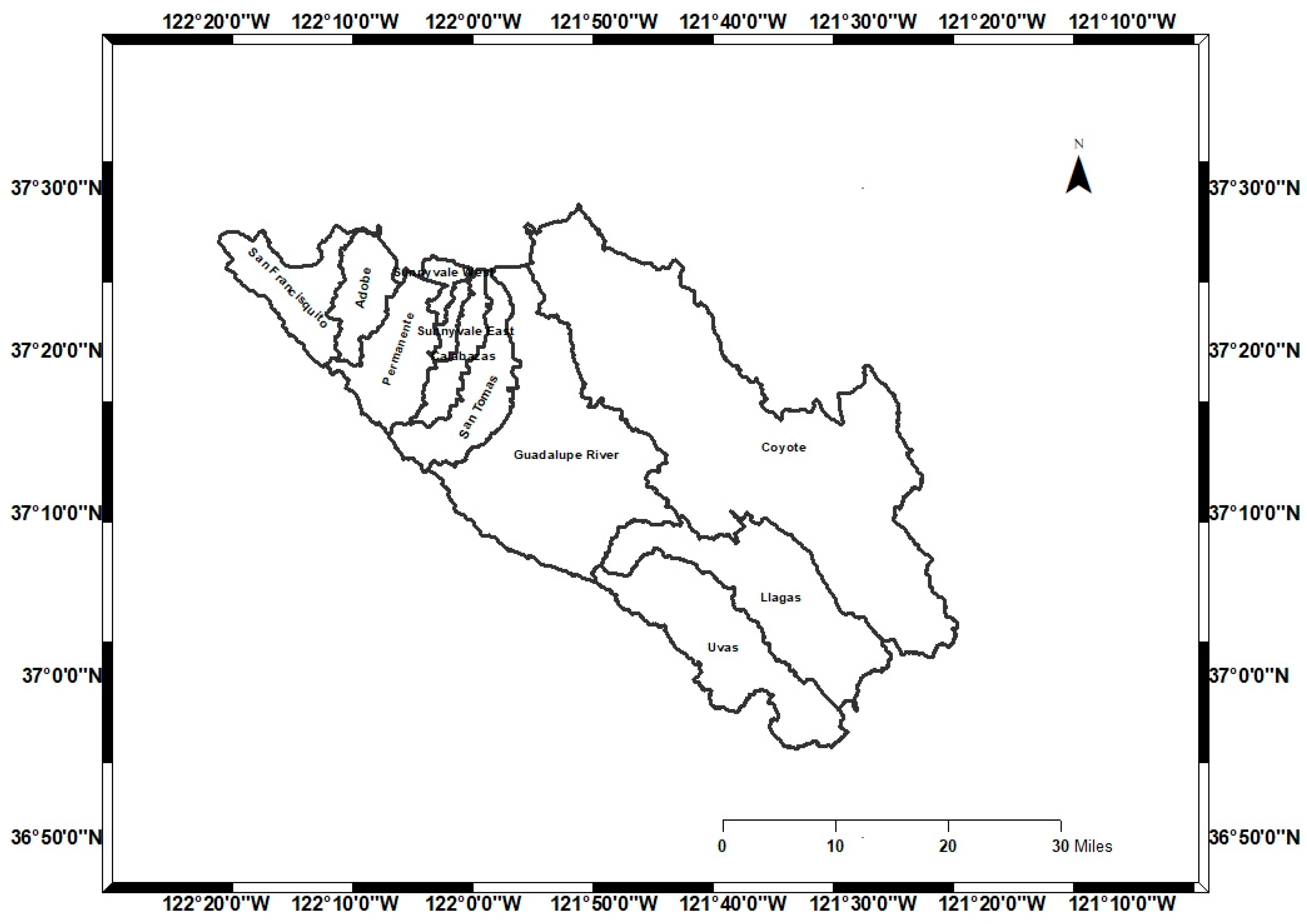
The Santa Clara Valley in California was used as the case study site for this analysis. The areal extent of the Santa Clara watershed area as shown in Figure 1 is 3713 Sq. Km. This region experiences a distinct Mediterranean climate, featuring warm, dry summers and mild, wet winters, which highly accentuate the seasonal thermal variations between natural and developed landscapes.

2.2. Data Used

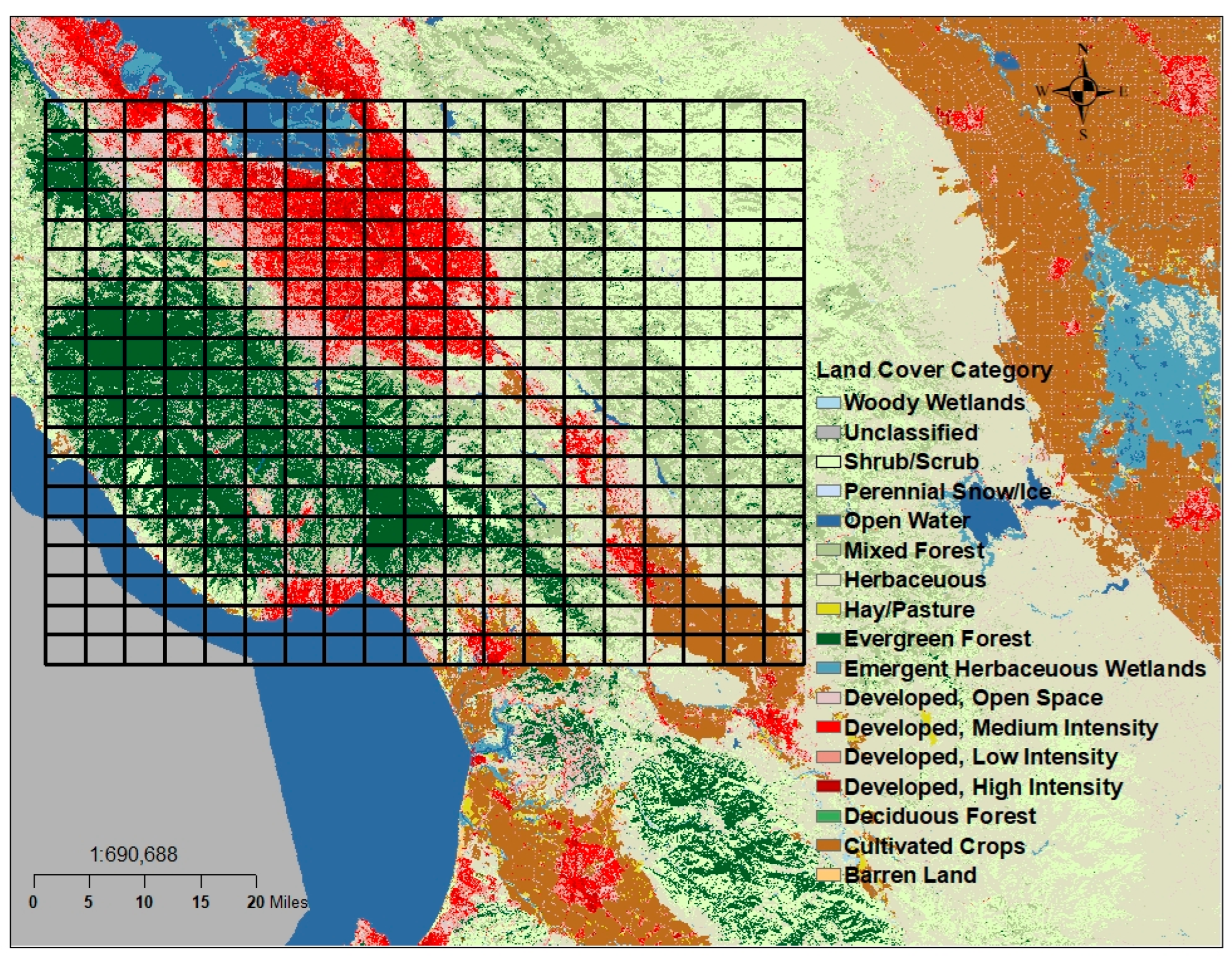
National Land Cover Data: NLCD maps obtained from the Multi-Resolution Land Characteristics Consortium (MRLC; https://www.mrlc.gov/) were used to evaluate the land cover categories across the grid framework. Spatial Analyst tools in Esri ArcMap 10.3 (Environmental Systems Research Institute, Inc., Redlands, CA, USA) were utilized to determine the land cover characteristics of each grid cell. Specifically, the Zonal Statistics tool was applied to compute the majority land cover category within each $5 \mathrm{km}\times 5 \mathrm{km}$ grid cell. The primary land cover categories selected for comparative analysis were residential, forest, agricultural, wetlands, and shrubs. Figure 2 illustrates the majority land cover distribution across the study area for the baseline year 2001. To account for dynamic land-use transitions and land cover changes across the multi-year study window, land cover classifications were assigned using temporally corresponding NLCD products for 2001, 2004, 2006, 2008, and 2011. The intermediate Landsat observation years were matched to the closest-preceding NLCD edition. Dynamically updating the land cover ensured that the surface temperature (LST) and fractional vegetation cover ($F_r$) evaluations accurately reflected active, real-time landscape conditions.

Landsat Surface Temperature and Surface Reflectance Data: Landsat 5 TM Collection 2 Level-2 Surface Temperature (_ST_B6) and Surface Reflectance products (Path 44/Row 34) were acquired from USGS EarthExplorer for June across the 2001–2011 multi-year observation period [14,15]. These products were atmospherically corrected and radiometrically calibrated according to official USGS Collection 2 processing protocols, incorporating internal scale factors, additive offsets, and single-channel thermal retrieval algorithms as detailed in official USGS technical documentation [14,15]. To maintain high data quality and eliminate atmospheric contamination, scene selection was strictly restricted to products with total scene cloud cover below 20%. June observations for 2007 and 2009 were excluded from the analysis because no scenes met this 20% cloud cover quality threshold.

Table 1. Landsat data information.

Year	Landsat 5 WRS Path and Row	Landsat Scene Acquisition Date	Cloud Cover Percentage
2001	Path = 44, Row = 34	18 June 2001	0%
2002	Path = 44, Row = 34	5 June 2002	0%
2003	Path = 44, Row = 34	24 June 2003	0%
2004	Path = 44, Row = 34	26 June 2004	7%
2005	Path = 44, Row = 34	13 June 2005	1%
2006	Path = 44, Row = 34	16 June 2006	0%
2008	Path = 44, Row = 34	5 June 2008	0%
2010	Path = 44, Row = 34	11 June 2010	0%
2011	Path = 44, Row = 34	14 June 2011	4%

summarizes the acquisition dates, path/row footprint, and cloud cover percentages across the nine analyzed observation years.

2.3. Methods

As the first step, 5 km × 5 km grids were generated for the Santa Clara County (SCC) watershed area. The $5 \mathrm{km}$ spatial resolution was selected to align local sub-pixel canopy dynamics with regional watershed planning boundaries and to maintain spatial compatibility with regional atmospheric models (e.g., the Weather Research and Forecasting (WRF) model), which routinely operate at $5 \mathrm{km}$ domain resolutions to simulate land–atmosphere energy exchange.

The total number of grids generated was 371. The National Land Cover Data (NLCD) obtained from the Multi-Resolution Land Characteristics Consortium was used in this study to determine the land cover category of each grid cell. The land cover category of each 5 km grid cell was computed using Esri’s ArcMap 10.3 Spatial Analyst Zonal Statistics Tool. Grid cells with the following land cover categories were used for the analysis: developed, low intensity and medium intensity; cultivated crops; forest; shrubs; and developed, open space. The total number of grid cells in the chosen land cover categories was 284.

Further, the mean surface temperature in each grid cell was computed using the ArcGIS Spatial Analyst Zonal Statistics Tool. Further, the Landsat Surface Temperature (ST) data in scaled Kelvin was processed in ArcMap for the month of June during the time period of 2001 through 2011.

2.3.1. Phase 1: Computation of NDVI

The Normalized Difference Vegetation Index (NDVI) is a measure of vegetation health, and its values range from −1 to +1. It is mathematically expressed as

$$NDVI={\displaystyle \frac{{\rho }_{\mathrm{NIR}}-{\rho }_{\mathrm{RED}}}{{\rho }_{\mathrm{NIR}}+{\rho }_{\mathrm{RED}}}}$$

(1)

In Landsat 5 data, the red and near-infrared reflectance correspond to Band 3 and Band 4; hence, the NDVI was calculated using Bands 4 and 3:

$$NDVI={\displaystyle \frac{\mathrm{Band} 4-\mathrm{Band} 3}{\mathrm{Band} 4+\mathrm{Band} 3}}$$

(2)

The NDVI tool in Esri’s ArcMap was used to compute the NDVI. The values of NDVI are pixel-level, with a spatial resolution of 30 m × 30 m. To align the vegetation metrics with the regional scale of analysis, the mean $NDVI$ value (${\mathrm{NDVI}}_{\mathrm{grid}}$) within each $5 \mathrm{km}\times 5 \mathrm{km}$ grid cell was aggregated using the Spatial Analyst Zonal Statistics tool in ArcMap.

2.3.2. Phase 2: Computation of Fractional Vegetation Cover ($F_{\mathrm{r}}$)

The fractional vegetation cover was calculated using the scaled index method proposed by [16]. To maintain spatial accuracy and avoid non-linear spatial aggregation errors ($F_r\left(\overline{\mathrm{NDVI}}\right)\ne \overline{F_r\left(\mathrm{NDVI}\right)}$), $F_r$ was calculated directly at native Landsat sensor resolution ($30 \mathrm{m}$) prior to zonal aggregation.

First, the surface reflectance (SR) bands were converted from Collection 2 Level 2 scaled integer Digital Numbers ($\mathrm{DN}\mathrm{s}$) to unitless surface reflectance ($SR=\mathrm{DN}\times 0.000025-0.2$). The native $30 \mathrm{m}$ NDVI rasters were then computed. Next, the normalized vegetation cover index values (${\mathrm{N}}^{*}\hspace{0.17em}$) were calculated at the pixel scale to isolate the canopy response between bare soil (${\mathrm{NDVI}}_{\mathrm{soil}}$) and full dense vegetation (${\mathrm{NDVI}}_{\mathrm{veg}}$) endmembers:

$${\mathrm{N}}^{\mathrm{*}}={\displaystyle \frac{\mathrm{NDVI}-{\mathrm{NDVI}}_{\mathrm{soil}}}{{\mathrm{NDVI}}_{\mathrm{veg}}-{\mathrm{NDVI}}_{\mathrm{soil}}}}$$

(3)

Standard regional operational thresholds were established at ${\mathrm{NDVI}}_{\mathrm{soil}}=0.05$ and ${\mathrm{NDVI}}_{\mathrm{veg}}=0.85$. These endmembers were verified via empirical spectral sampling across representative land cover targets in the Santa Clara Valley during early June scenes. Unvegetated bare soil, dry foothill terrain, fallow agricultural plots, and impervious urban surfaces confirmed ${\mathrm{NDVI}}_{\mathrm{soil}}=0.05$ as an appropriate regional bare soil baseline. The upper threshold (${\mathrm{NDVI}}_{\mathrm{veg}}=0.85$) was defined by dense, fully irrigated urban green spaces, municipal parks, golf courses, and closed forest canopies.

The pixel-level fractional vegetation cover ($F_r$) was then computed as the square of the normalized value as proposed by [14]:

$$F_r={\left({\mathrm{N}}^{*}\right)}^2={\left({\displaystyle \frac{\mathrm{NDVI}-{\mathrm{NDVI}}_{\mathrm{soil}}}{{\mathrm{NDVI}}_{\mathrm{veg}}-{\mathrm{NDVI}}_{\mathrm{soil}}}}\right)}^2$$

(4)

Pixels exhibiting $\mathrm{NDVI}\le {\mathrm{NDVI}}_{\mathrm{soil}}$ were bounded to $F_r=0.0$, while pixels exceeding the ${\mathrm{NDVI}}_{\mathrm{veg}}$ were set to $F_r=1.0$. Once computed at the native $30 \mathrm{m}$ resolution, the pixel-level $F_r$ rasters were spatially averaged across each $5 \mathrm{km}\times 5 \mathrm{km}$ grid cell using zonal statistics (ZonalStatisticsAsTable), yielding the zonal mean fractional vegetation cover ($F_r$) for each land cover class and analysis year.

To evaluate the potential uncertainty associated with selecting the fixed endmember thresholds, an endmember sensitivity analysis was conducted following [17]. The bare soil endmember was systematically evaluated across $\left[0.00,0.05,0.10\right]$ and the dense canopy endmember across $\left[0.80,0.85,0.90\right]$. Because $F_r$ scales monotonically with NDVI, adjusting the operational endmembers rescaled the absolute numerical values without altering the underlying spatial variance structure, statistical significance (p < 0.001), or directional inverse slope of the LST–$F_r$ relationship.

2.4. Land Surface Temperature (LST) Derivation and Scaling

Landsat 5 TM Collection 2 Level-2 Surface Temperature products (_ST_B6) were processed to evaluate the land cover thermal responses across the study period. Cloud-contaminated observations, open water, and invalid pixels identified in the Level-1 Pixel Quality (QA_PIXEL) and Level-2 Surface Temperature Quality (ST_QA) bands were masked prior to statistical extraction.

For each observation year, the mean Digital Number (${\mathrm{DN}}_{\mathrm{mean}}$) was calculated across all valid pixels within each target land cover category and 5 km grid cell using the Esri ArcMap Spatial Analyst Zonal Statistics tool. The aggregated ${\mathrm{DN}}_{\mathrm{mean}}$ values were converted to scaled Kelvin ($T_{\mathrm{Kelvin}}$) using the official USGS Collection 2 Level-2 scale factor (0.00341802) and additive offset (149.0):

$$T_{\mathrm{Kelvin}}=\left({\mathrm{DN}}_{\mathrm{mean}}\times 0.00341802\right)+149.0$$

The resulting scaled Kelvin temperatures were subsequently converted to degrees Fahrenheit (°F) for regional microclimate evaluation:

$$\mathrm{LST}\left(°\mathrm{F}\right)=\left(T_{\mathrm{Kelvin}}-273.15\right)\times {\displaystyle \frac{9}{5}}+32$$

Because the USGS calibration and unit conversion equations are strictly linear transformations, calculating the zonal mean DNs prior to applying the scale factors and unit conversions is mathematically equivalent to a pixel-by-pixel transformation prior to averaging.

2.5. Statistical Regression Analysis

A pooled Ordinary Least Squares (OLS) regression model was executed across the compiled matrix of 45 category–year observations (5 land cover categories × 9 study years):

$${\mathrm{LST}}_{i,t}={\beta }_0+{\beta }_1{\left({\overline{F}}_r\right)}_{i,t}+{ϵ}_{i,t}$$

where the ${\mathrm{LST}}_{i,t}$ and ${\left({\overline{F}}_r\right)}_{i,t}$ represent the mean land surface temperature (°F) and mean fractional vegetation cover of land cover category i in year t. The model parameters evaluate the overall thermal sensitivity (${\beta }_1$, °F per unit $F_r$) and baseline surface temperature (${\beta }_0$) across the regional landscape over the decade.

3. Results

3.1. Endmember Sensitivity Analysis for Fr Computation

Seven separate OLS regression models were independently executed across the tested endmember threshold combinations (

Table 2. Sensitivity analysis of pooled OLS regression parameters across varying soil (${\mathrm{NDVI}}_{\mathrm{soil}}) \mathrm{a}\mathrm{n}\mathrm{d} \mathrm{d}\mathrm{e}\mathrm{n}\mathrm{s}\mathrm{e} \mathrm{c}\mathrm{a}\mathrm{n}\mathrm{o}\mathrm{p}\mathrm{y} ({\mathrm{NDVI}}_{\mathrm{veg}}$) endmember thresholds ($N=45$).

Scenario/Configuration	NDVIsoil	NDVIveg	Dynamic Range (ΔNDVI)	Intercept (β0)	Cooling Slope (β1)	R2	F-Statistic	p-Value
Baseline (Primary Model)	0.05	0.85	0.80	108.921	−38.259	0.5109	44.91	3.48 × 10−8
Conservative Soil	0.00	0.85	0.85	108.921	−43.191	0.5109	44.91	3.48 × 10−8
High Soil Threshold	0.10	0.85	0.75	108.921	−33.626	0.5109	44.91	3.48 × 10−8
Low Vegetation Threshold	0.05	0.80	0.75	108.921	−33.626	0.5109	44.91	3.48 × 10−8
High Vegetation Threshold	0.05	0.90	0.85	108.921	−43.191	0.5109	44.91	3.48 × 10−8
Shifted Range (Low)	0.00	0.80	0.80	108.921	−38.259	0.5109	44.91	3.48 × 10−8
Shifted Range (High)	0.10	0.90	0.80	108.921	−38.259	0.5109	44.91	3.48 × 10−8

Note: Each row represents an independent Ordinary Least Squares (OLS) regression model ($N=45$) fitted separately to the re-calculated $F_r$ dataset under the specified endmember thresholds.

). The pooled OLS regression model demonstrated mathematical invariance across all tested endmember threshold combinations. Across all seven scenarios, the proportion of explained surface temperature variance ($R^2=0.5109$), overall model fit ($F=44.91$), statistical significance ($p=3.48\times {10}^{-8}$), and non-vegetated intercept (${\beta }_0=108.921$ °F) remained identical. The cooling slope (${\beta }_1$) scaled predictably relative to the effective NDVI dynamic range ($\Delta \mathrm{NDVI}={\mathrm{NDVI}}_{\mathrm{veg}}-{\mathrm{NDVI}}_{\mathrm{soil}}$), ranging between $-33.626$ °F ($\Delta \mathrm{NDVI}=0.75$) and $-43.191$ °F ($\Delta \mathrm{NDVI}=0.85$) per unit $F_r$.

3.2. Spatio-Temporal Variations in LST Across Land Covers

The mean LST values were quantified for the month of June across the 2001–2011 observation window within a 5 km grid framework of the Santa Clara County watershed.

Table 3. Mean LST values across various land cover categories in Fahrenheit (°F).

Land Cover Category	2001	2002	2003	2004	2005	2006	2008	2010	2011
Forest	71.10	95.23	81.67	84.17	88.52	90.81	80.94	78.94	86.06
Developed, Open Space	85.26	104.43	94.56	96.63	101.12	101.13	90.78	91.92	95.73
Shrubs	82.21	106.89	93.78	102.09	98.95	100.78	96.62	89.03	98.59
Cultivated Crops	91.41	111.65	100.42	102.79	106.52	105.80	101.57	97.94	105.91
Developed, Low and Medium Intensity	95.73	111.14	102.72	103.74	109.74	108.29	101.06	100.19	105.77

and Figure 3 present the empirical mean Fahrenheit (°F) values derived for each of the five core land cover zones: forest; developed open space; shrubs; cultivated crops; and developed, low and medium intensity.

The empirical data establishes a consistent thermal hierarchy throughout the monitored decade:

• Developed, low- and medium-intensity areas consistently exhibited the highest baseline thermal signatures, reaching a study period maximum of 111.14 °F in June 2002.
• Forest zones continuously recorded the lowest surface temperatures, dropping to a study minimum of 71.10 °F in June 2001 and remaining between 16 °F and 25 °F cooler than the adjacent developed areas in any given year.
• Cultivated Crops tracked closely with the built environments during the early summer season, reaching a peak signature of 111.65 °F in 2002.
• Shrubs and developed, open space occupied intermediate thermal ranks, peaking in 2002 at 106.89 °F and 104.43 °F, respectively.

3.3. Multi-Year Land Cover Characterization

The multi-year zonal aggregation revealed distinct structural differences in vegetation density and thermal regime across the five land cover classes (

Table 4. Multi-year mean fractional vegetation cover (${\mathrm{F}}_{\mathrm{r}}$) and land surface temperature (LST) across land cover categories (2001–2011).

Land Cover Category	Mean Fr (2001–2011)	Mean LST (°F)
Developed, Low & Medium Intensity	0.1471	104.26
Cultivated Crops	0.1743	102.67
Shrubs/Scrub	0.2997	96.55
Developed, Open Space	0.3546	95.73
Forest	0.625	84.16

). The forested grid cells maintained the highest fractional vegetation cover ($F_r=0.625$) and lowest mean surface temperatures (84.16 °F). In contrast, the low- and medium-intensity developed areas exhibited the lowest vegetation cover ($F_r=0.147$) and highest mean temperatures (104.26 °F).

3.4. Primary Regional Regression Model ($N=45$)

Pooling all 45 data points into a single regional OLS model as shown in Figure 4 yielded a statistically significant inverse linear relationship between the vegetation cover and land surface temperature:

$$\mathrm{LST}=108.921-38.259\left(F_r\right)\hspace{1em}\left(R^2=0.5109,\hspace{0.17em}F=44.91,\hspace{0.17em}p=3.48\times {10}^{-8}\right)$$

(5)

The baseline surface temperature parameter (${\beta }_0=108.921$ °F) indicates the expected thermal state of non-vegetated surfaces ($F_r=0$). The global cooling slope (${\beta }_1=-38.259$ °F) demonstrates that every 0.10 (10%) increase in the zonal fractional vegetation cover yields an average surface temperature drop of approximately 3.83 °F across the regional domain. The variations in $F_r$ account for 51.1% of the total variance in the surface temperature across land cover classes and study years.

3.5. Long-Term Category Baseline Model ($N=5$)

Evaluating the long-term category means ($N=5$) eliminated interannual weather fluctuations, isolating the structural cooling capacity of land cover composition:

$$\mathrm{LST}=109.921-41.381\left(F_r\right)\hspace{1em}\left(R^2=0.9945,\hspace{0.17em}p=1.71\times {10}^{-4}\right)$$

(6)

At the category baseline level, the vegetation density explains $99.45\%$ of the variation in the mean surface temperature between land-use classes, confirming that the structural vegetation cover is the dominant driver of inter-category surface climate variation.

4. Discussion

4.1. Thermal Mitigation Efficiency Across the Land Cover Gradient

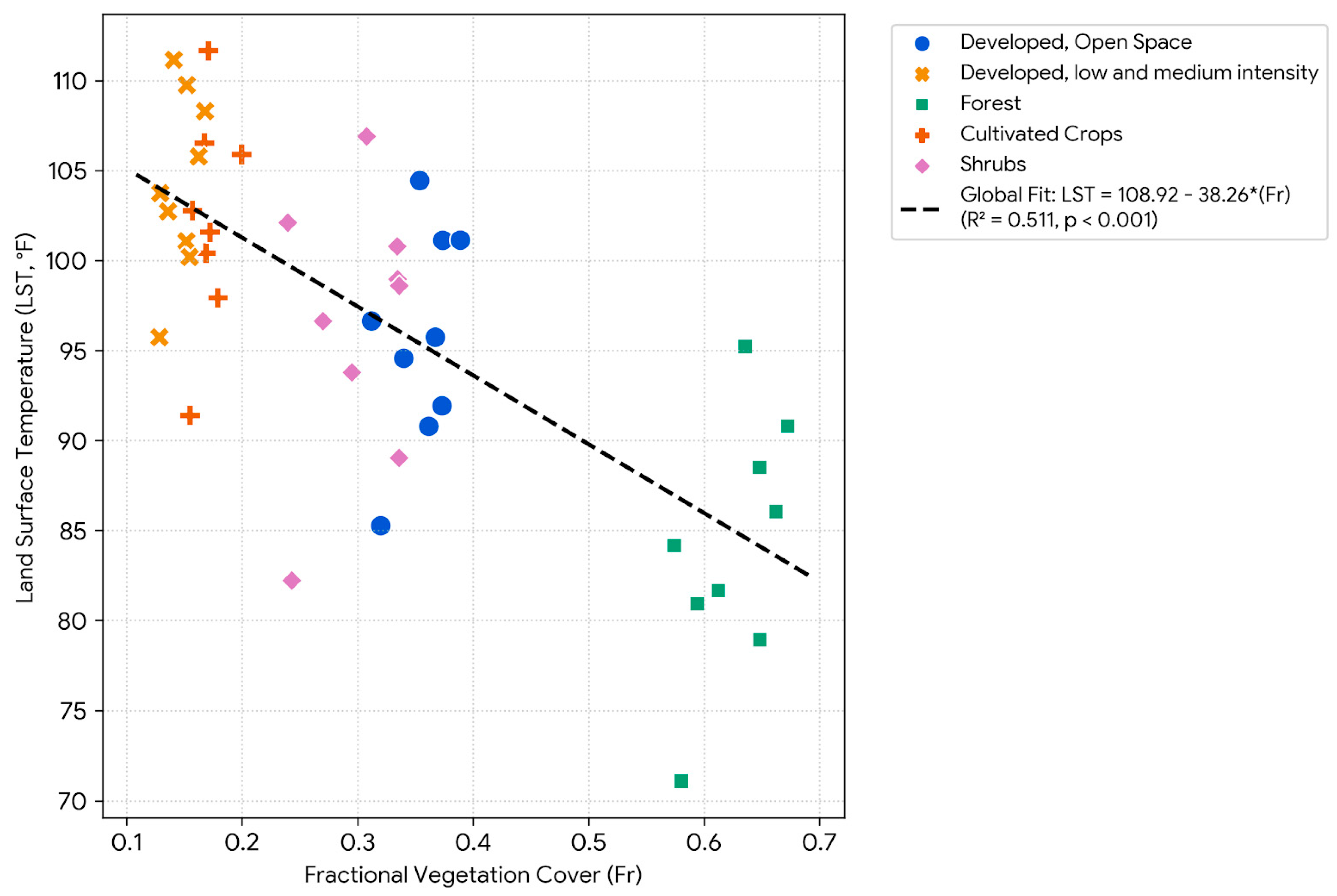
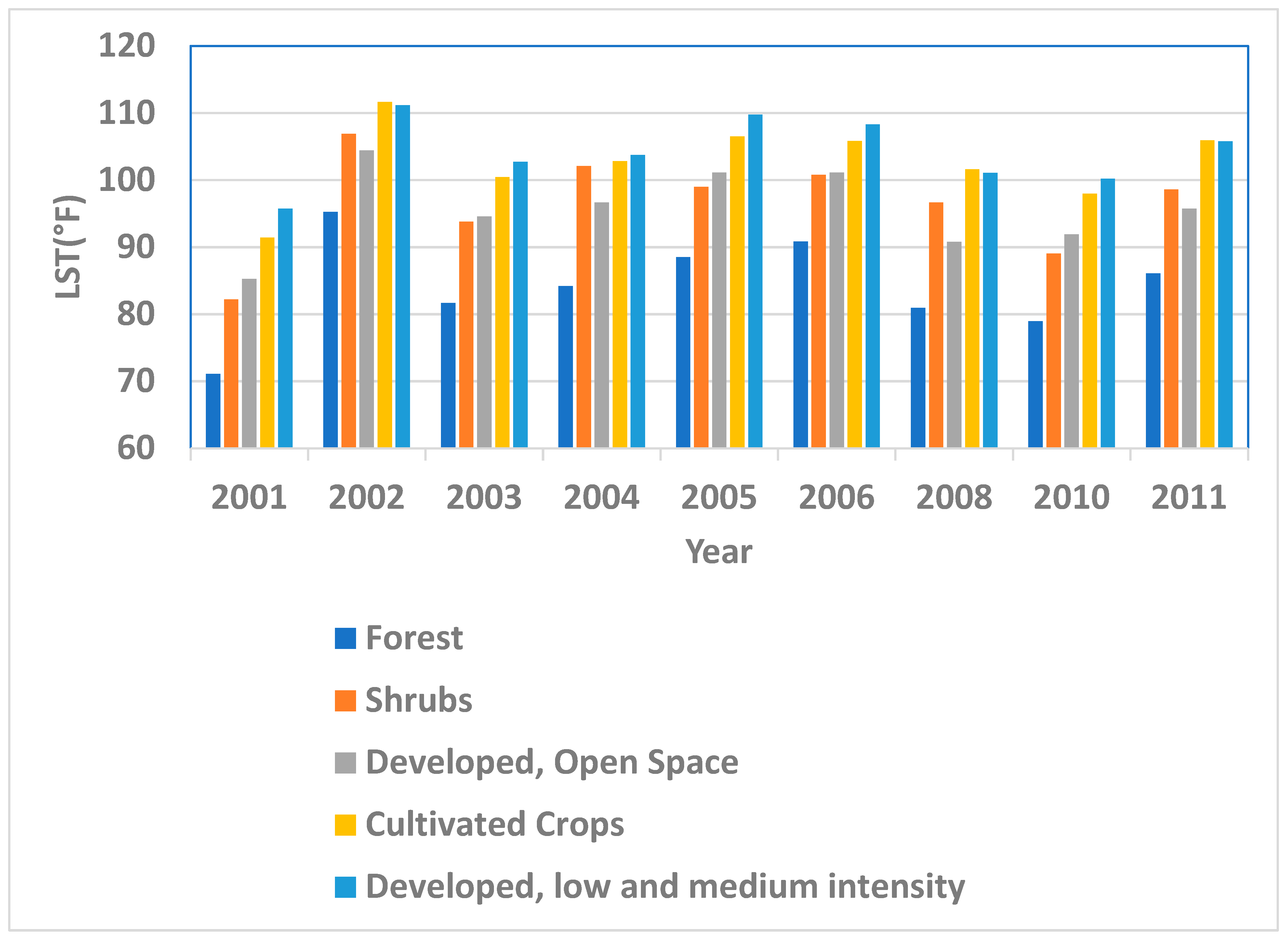
The strong inverse linear relationship (${\beta }_1=-38.259 °\mathrm{F}/F_r$) confirms the efficacy of vegetative canopy expansion for suppressing regional land surface temperatures. Comparing the land cover categories highlights the decisive role of structural canopy architecture: the high-density forest cover ($F_r=0.625$, $\mathrm{LST}=84.16$ °F) delivers a 20.10 °F surface temperature reduction relative to the low- and medium-intensity developed zones ($F_r=0.147$, $\mathrm{LST}=104.26$ °F).

Crucially, the developed, open space (${\mathrm{F}}_{\mathrm{r}}=0.355$, $\mathrm{LST}=95.73$ °F) achieves an 8.53 °F cooling effect compared to low/medium developed areas (${\mathrm{F}}_{\mathrm{r}}=0.147$). This demonstrates that incorporating managed green infrastructure (e.g., parks, urban forests, and lawn spaces) within developed environments yields substantial microclimatic relief even without complete canopy restoration.

4.2. Physical Mechanisms and Physiological Controls

While $F_r$ serves as an indicator of canopy spatial abundance, the surface thermal regulation is also mediated by the vegetation’s physiological state, hydrological availability, and canopy structure. In California Mediterranean climates, early-summer agricultural surfaces (Cultivated Crops, $\mathrm{LST}=102.67$ °F) exhibit elevated surface temperatures despite moderate vegetation indices. This behavior is consistent with fallow ground, recent harvesting, or reduced soil moisture availability, which limit the latent heat flux via evapotranspiration. As demonstrated by [18], water availability strongly controls the vegetation cooling capacity.

Additionally, the thermal response of mature woody vegetation reflects complex energy balance dynamics, including canopy shading, stomatal resistance, and root coupling with subsurface hydrologic reservoirs. Recent field studies [19] have indicated that mature tree canopies experience thermal buffering mediated by deep soil coupling and internal sapwood heat storage. Consequently, the empirical slope (${\beta }_1=-38.259$ °F) should be interpreted as an observational association within the fitted dataset rather than a universal cooling efficiency.

4.3. Methodological Considerations and Model Interpretation ($R^2=0.5109$)

The pooling observations across nine study years ($N=45$) incorporate the interannual climate variation (e.g., warmer vs. cooler summer baselines) while evaluating the regional relationship across consolidated land cover categories.

The resulting pooled OLS model,

$$\mathrm{LST}=108.921-38.259\left(F_r\right)\hspace{1em}\left(R^2=0.5109,\hspace{0.17em}F=44.91,\hspace{0.17em}p=3.48\times {10}^{-8}\right)$$

provides a multi-year empirical summary of regional surface thermal association. When aggregated to multi-year category baselines ($N=5$), the model accounts for 99.45% of the inter-category variance ($R^2=0.9945$), confirming that vegetation cover differences represent the primary structural driver among land cover thermal baselines. Unmeasured covariates—such as surface albedo, soil moisture, distance to San Francisco Bay, and micro-scale meteorological variation—account for the remaining variance in the pooled dataset. Aggregating the $30 \mathrm{m}$ pixel $F_r$ values to 5 km zonal grids effectively filters the micro-scale background noise while maintaining high statistical significance ($F=44.91,\hspace{0.17em}p<0.001$) across the regional domain. Crucially, a $5 \mathrm{km}\times 5 \mathrm{km}$ spatial grid framework directly aligns with the domain resolution routinely used in regional climate and numerical weather prediction models, such as the Weather Research and Forecasting (WRF) model. Utilizing a 5 km grid size ensures that the derived empirical $F_r$–LST parameterizations can be seamlessly integrated as surface input parameters or validation baselines in meso-scale atmospheric simulations.

Furthermore, the endmember sensitivity analysis confirms that the threshold selection does not introduce systematic bias or alter the substantive findings of this study. Because $F_r$ is a monotonic linear transformation of scaled NDVI squared, adjusting the endmember bounds modifies the numerical scaling of $F_r$ without altering the relative rank order or variance structure of the data matrix. Consequently, the proportion of thermal variance explained ($R^2=0.5109,\hspace{0.17em}p<0.001$) and the baseline unvegetated temperature (108.921 °F) are invariant to threshold adjustments. While the empirical cooling rate (${\beta }_1$) adjusts in proportion to the dynamic range ($\Delta \mathrm{NDVI}$ range from 0.75 to 0.85), the negative direction, statistical significance, and land cover thermal hierarchy remain stable. This stability demonstrates that the operational endmembers (${\mathrm{NDVI}}_{\mathrm{soil}}=0.05$; ${\mathrm{NDVI}}_{\mathrm{veg}}=0.85$) provide a reliable baseline for regional thermal assessments in the Santa Clara Valley.

4.4. Implications for Urban Planning Contexts

The observational association between an increased $F_r$ and reduced LST provides empirical support consistent with urban greening strategies. Urban planners and municipal managers can use these empirical relationships as contextual baselines when evaluating green infrastructure interventions. For instance, increasing the fractional vegetation cover ($F_r$) by 0.15 (15%) within residential or commercial districts is estimated to reduce surface temperatures by approximately 5.74 °F. However, local heat mitigation effectiveness will depend on plant species selection, irrigation management, structural canopy design, and localized urban morphology.

5. Conclusions

This study evaluated the longitudinal (2001–2011) relationship between the fractional vegetation cover ($F_r$) and land surface temperature (LST) across a 5 km spatial grid framework stratified into five primary land cover categories in the Santa Clara Valley. A pooled Ordinary Least Squares regression model (N = 45) established the following empirical association:

$$\mathrm{LST}=108.921-38.259\left(F_r\right)\hspace{1em}\left(R^2=0.5109,\hspace{0.17em}F=44.91,\hspace{0.17em}p=3.48\times {10}^{-8}\right)$$

The fractional vegetation cover ($F_r$) accounts for 51.09% of the variance in surface temperature across the pooled dataset, while the multi-year category baseline means exhibit an exceptional $R^2$ of 0.9945. These findings document a clear inverse association between vegetation abundance and land surface temperature, offering a baseline framework for informing urban climate adaptation and green infrastructure planning.