A Two-Dimensional Shallow-Water Model for Pluvial Flood Analysis in Urban Areas ^†

Abstract

Urban flood simulation requires numerical models capable of representing the two-dimensional propagation of water over topographically complex surfaces under intense rainfall and localized inflows. The paper presents a two-dimensional hydraulic model based on the Saint-Venant equations (shallow-water equations). The numerical model uses a Rusanov-type flux and operates on raster-based digital elevation models (DEMs). Notably, it allows for the modeling of both spatially distributed rainfall over the domain (rain-on-grid approach) and multiple independent point sources representing urban drainage system surcharging or overflow, each associated with a specific discharge hydrograph. The results confirm the model’s reliability for urban hydraulic hazard assessments.

1. Introduction

Urban pluvial flooding occurs when short-duration, high-intensity rainfall generates runoff that cannot be conveyed rapidly enough through drainage networks, or infiltrate into the soil. These events are typically flash floods, owing to their rapid onset and strong spatial localization, especially within densely built environments. Their small temporal and spatial scales make pluvial floods significantly harder to forecast and map than riverine or coastal flooding, as highlighted by the UK Environment Agency [1]. Although pluvial flooding may also affect rural areas, it is predominantly an urban phenomenon, where surface sealing, limited infiltration, and the concentration of exposed assets amplify its impacts.

Recent assessments indicate that nearly two million residents in urban areas of the United Kingdom face an annual 0.5% probability of experiencing pluvial flooding, equivalent to a 1-in-200-year event. This accounts for about 5% of the total urban population and represents nearly one-third of the flood risk from all sources. The projections for 2050 suggest that the number of people exposed could rise to 3.2 million, due to the combined effects of climate change (approximately +300,000 people) and population growth (+900,000). Because pluvial floods often occur with minimal warning in locations not traditionally considered flood-prone, they are sometimes referred to as an “invisible hazard” [2].

In urban environments, pluvial flooding takes place when intense rainfall overwhelms the capacity of the sewer network, minor urban watercourses, or surface drainage features, causing water to pond on streets and potentially enter buildings [3]. This definition encompasses three interconnected processes:

• Direct surface runoff;
• Surcharge and overflow from the sewer system;
• Flooding from small urban watercourses.

These mechanisms are intrinsically linked and must be analyzed together for reliable flood modeling and risk assessment.

During heavy rainfall, a thin layer of runoff develops before the surface flow becomes fully established. The initial water film is extremely shallow, fractions of a millimeter on impervious surfaces and a few millimeters on vegetated areas [4]. The runoff then follows topographic pathways such as streets, alleys, and open channels, eventually reaching either an urban watercourse or a drainage inlet (e.g., gullies or manholes) that provides access to the piped network.

Urban pluvial flooding is therefore a complex, dynamic process governed by rainfall intensity, surface characteristics, and the hydraulic performance of urban drainage systems. Its growing relevance underscores the need for improved modeling approaches and integrated urban water management strategies capable of addressing the increasing pressures posed by climate change and urban expansion.

In the present study, a two-dimensional hydraulic model based on the Saint-Venant equations (shallow-water equations), solved through a first-order explicit finite-volume scheme, is proposed. The numerical method employs a Rusanov-type flux, ensuring numerical stability, mass conservation, and the robust handling of wetting and drying conditions. Dissipative effects are accounted for through a semi-implicit formulation of Manning friction. An application to a real-world urban flooding event yields maximum inundation depth maps and arrival times consistent with the flow patterns reported in the literature. The results confirm the model’s reliability for urban hydraulic hazard assessments.

2. Model Description

The simulation model solves the shallow-water equations (Saint-Venant equations) in two horizontal dimensions, 2D_SWE. These are a set of hyperbolic conservation laws representing the conservation of mass (continuity) and momentum in the x and y directions. In the conservative form, the state vector U = [h; hu; hv] comprises the water depth h and the two components of momentum hu and hv (with u and v being the depth-averaged velocities).

Its objective is to update, in a conservative and stable manner, water depth $h$, and depth-integrated momenta $hu$ and $hv$, while accounting for bed topography, rainfall and point inflows, wetting and drying, bottom friction, and open boundary conditions.

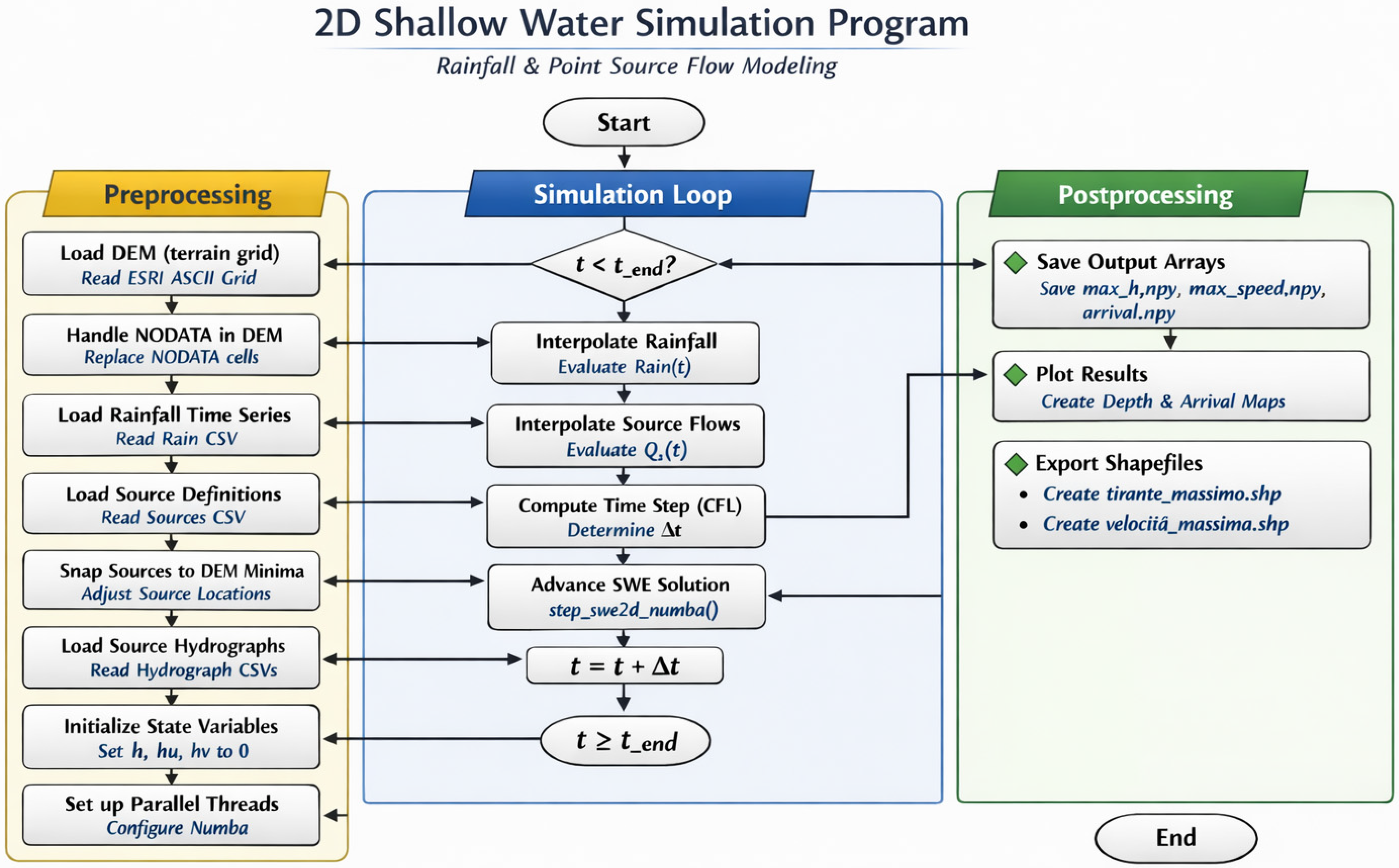
The implementation follows a finite-volume, Godunov-type approach, designed for robustness on complex topography and partially dry domains (Figure 1). The governing equations can be written as follows:

$$\begin{gathered} {\displaystyle \frac{\partial h}{\partial t}}+{\displaystyle \frac{\partial \left(hu\right)}{\partial x}}+{\displaystyle \frac{\partial \left(hv\right)}{\partial y}}=R\left(x,y,t\right) \\ {\displaystyle \frac{\partial \left(hu\right)}{\partial t}}+{\displaystyle \frac{\partial }{\partial x}}\left(h{u}^2+{\displaystyle \frac{1}{2}}g{h}^2\right)+{\displaystyle \frac{\partial \left(huv\right)}{\partial y}}=-gh{\displaystyle \frac{\partial z}{\partial x}}-{\tau }_x \\ {\displaystyle \frac{\partial \left(hv\right)}{\partial t}}+{\displaystyle \frac{\partial \left(hvu\right)}{\partial x}}+{\displaystyle \frac{\partial }{\partial y}}\left(h{v}^2+{\displaystyle \frac{1}{2}}g{h}^2\right)=-gh{\displaystyle \frac{\partial z}{\partial y}}-{\tau }_y \end{gathered}$$

(1)

where:

-

$z\left(x,y\right)$ is the bed elevation;

-

$R$ is the source term represented by rainfall (mm/h), and point-source inflows;

-

${\tau }_x,{\tau }_y$ are friction terms;

-

$g$ is the gravitational acceleration.

Figure 1. Flowchart of the entire tool.

Figure 1. Flowchart of the entire tool.

The computational domain is discretized into rectangular cells. Each cell stores cell-averaged values of $h$, $hu$, and $hv$.

The update over a time step Δt follows the standard finite-volume form:

$$U_{i,j}^{n+1}=U_{i,j}^n-{\displaystyle \frac{\Delta t}{\Delta x}}(F_{i+1/2,j}-F_{i-1/2,j})-{\displaystyle \frac{\Delta t}{\Delta y}}(G_{i,j+1/2}-G_{i,j-1/2})+\Delta t\hspace{0.17em}S$$

(2)

where:

$- F$ and $G$ are numerical fluxes;

$- S$ collects the source terms (rainfall, inflows, and friction).

Topography introduces source terms that can destroy the equilibrium if not handled carefully. To preserve the lake-at-rest condition (zero velocity, and constant free surface), the solver applies hydrostatic reconstruction at every cell interface.

At an interface, the following are carried out:

-

The maximum bed elevation is identified:

$$z^{\ast }=\mathrm{m}\mathrm{a}\mathrm{x}(z_L,z_R)$$

(3)

-

The reconstructed water depths are computed:

$$h_L^{\ast }=\max \left(0,h_L+z_L-z^{\ast }\right)h_R^{\ast }=\max \left(0,h_R+z_R-z^{\ast }\right)$$

(4)

This ensures the exact balance between the pressure and bed slope, the non-negative reconstructed depths, and, finally, the correct treatment of partially dry interfaces. This approach follows the well-balanced strategy introduced by Audusse et al. [5].

At each interface, fluxes are computed using a Rusanov (local Lax–Friedrichs) solver. For each interface, the following are carried out:

-

Physical fluxes are computed from left and right reconstructed states;

-

The maximum wave speed is estimated:

$$s_{\mathrm{m}\mathrm{a}\mathrm{x}}=\mathrm{m}\mathrm{a}\mathrm{x}(\mid u\mid +\sqrt{gh})$$

(5)

-

The numerical flux is defined as follows:

$$F={\displaystyle \frac{1}{2}}(F_L+F_R)-{\displaystyle \frac{1}{2}}{s}_{\mathrm{m}\mathrm{a}\mathrm{x}}(U_R-U_L)$$

(6)

This choice guarantees stability, handles shocks and hydraulic jumps robustly, and is particularly reliable in wet–dry transitions. Even if this approach is more diffusive than Roe solvers, Rusanov fluxes are widely used in flood modeling for their robustness; thus, this is an upwind scheme that has the lowest explicit level of upwinding [6].

Accurately simulating wetting and drying processes—i.e., the movement of shorelines or boundaries between inundated and non-inundated areas—remains one of the most delicate aspects of solving the shallow-water equations. The model incorporates several numerical strategies to ensure a stable and physically consistent handling of wet/dry interfaces.

The first key component is the hydrostatic reconstruction, previously discussed, which guarantees that the reconstructed water depths remain non-negative. By enforcing this constraint, cells containing no water contribute zero flux, preventing non-physical exchanges between wet and dry regions.

In addition, the model introduces a small threshold depth, $h_{\mathrm{m}\mathrm{i}\mathrm{n}}$ (typically ${10}^{-4}\hspace{0.17em}\mathrm{m}$), to distinguish wet cells from dry ones. This threshold is used strictly for stability purposes. Cells with $h\le h_{\mathrm{m}\mathrm{i}\mathrm{n}}$ are treated as dry: their momentum components are explicitly set to zero, and they do not exchange fluxes with neighboring cells, except possibly as passive receivers of inflow.

This treatment is applied at two critical stages of the computation:

1.

Before flux evaluation, after the addition of rainfall or external sources. The algorithm loops through all cells and sets the following:

$$hu=hv=0 \mathrm{whenever} h\le h_{\mathrm{m}\mathrm{i}\mathrm{n}}.$$

This prevents the development of spurious velocities that would otherwise arise from dividing by extremely small water depths.

2.

After the flux update, once the new water depth $h_{\mathrm{new}}$ has been computed. If $h_{\mathrm{new}}\le h_{\mathrm{m}\mathrm{i}\mathrm{n}}$, the updated momentum values are again set to zero.

This ensures that a cell that becomes dry during the time step does not retain residual momentum that could produce non-physical “ghost” flows.

Such momentum clamping in nearly dry cells is widely adopted in shallow-water solvers to preserve numerical stability and physical realism in wetting–drying scenarios, and it is consistent with the approaches documented in the literature [7].

The model also enforces a positivity constraint on water depth: any small negative value that may arise from the numerical round-off or truncation errors is reset to zero. This correction is essential when using explicit schemes, as finite-precision arithmetic can occasionally produce slightly negative depths even when fluxes are physically conservative.

Together, the hydrostatic reconstruction, the positivity preservation, and the momentum resetting mechanism form a robust and reliable drying algorithm. As water recedes and the depth approaches the threshold $h_{\mathrm{m}\mathrm{i}\mathrm{n}}$, the model naturally transitions the cell into a dry state, halting all outgoing fluxes. The cell remains dry until it is reactivated by precipitation or by incoming flux from neighboring wet cells. This yields a stable and physically coherent representation of wetting and drying dynamics on complex, evolving free-surface domains.

Physically, h_min is a tolerance (on the order of millimeters) below which water is not tracked—any such tiny depth is considered zero to avoid instability. The value is chosen small enough to not affect mass conservation significantly, but large enough to avoid division by extremely small depths (herein, 10⁻⁴ m is used by default). This threshold, along with the well-balanced flux, prevents the common issue of “ringing” or oscillations at the shoreline.

Rainfall is treated as a source term in the continuity equation:

$$h^{n+1}=h^n+R\Delta t$$

(7)

This is applied uniformly over all cells, and no momentum is added (the rainfall is assumed to be vertically incident). Point inflows (e.g., sewer surcharges, and inflow hydrographs) are injected as volume:

$$\Delta h={\displaystyle \frac{Q\Delta t}{\Delta x\Delta y}}$$

(8)

Optionally, the inflow can be distributed over a 3 × 3 stencil to avoid local instabilities.

The time step Δt is computed dynamically using a CFL criterion:

$$\Delta t=\mathrm{CFL}\cdot \min ({\displaystyle \frac{\Delta x}{|u|+\sqrt{gh}}},{\displaystyle \frac{\Delta y}{|v|+\sqrt{gh}}})$$

(9)

This guarantees that no information propagates more than one cell per time step, maintaining the stability of the explicit scheme. All domain boundaries are treated as open (Neumann) boundaries with zero normal gradient and implemented by copying interior cell values to boundary cells. This allows waves and floodwater to exit the domain without artificial reflection.

Bottom friction is applied as a source term on momentum using Manning’s law:

$$\tau =g{n}^2{\displaystyle \frac{\mid U\mid }{h^{4/3}}}$$

(10)

The update is performed semi-implicitly:

$$U^{n+1}={\displaystyle \frac{U^n}{1+\tau \Delta t}}$$

(11)

This approach is stable even for shallow depths, and avoids severe time step reductions, while correctly damping velocities over rough terrain.

The entire code is then parallelized using Numba (Figure 1), which allows Python code to approach the speed of low-level languages for array-heavy computations. The @njit (parallel = True) operator on the Python (2025) code hints that Numba can auto-parallelize the outer loops. Indeed, the code uses prange (parallel range) for loops over the grid, enabling the multi-core execution of those loops. For example, the loop over all cells for the rainfall addition is parallelized, as are the loops for flux calculations in x and y, and the update loops over cells. This means each iteration (each row’s computation, for instance) can run concurrently on separate CPU threads. In practice, the code sets the number of threads (in this case, 16) and then compiles the step function at runtime on the first call. Once compiled, each step is executed in parallel, making it feasible to simulate large grids (millions of cells) with a reasonable speed. The parallelization strategy is highly beneficial for simulating 2D floods, as the computation of fluxes and updates is by far the most expensive part of the model. By leveraging multiple cores, the model achieves a near-linear speedup with the number of threads (until memory bandwidth becomes the bottleneck). In summary, the use of Numba allows the Python implementation to run at speeds comparable to compiled code, enabling fine-resolution and large-domain shallow-water simulations without sacrificing the convenience of Python for setup and I/O. The numerical scheme itself (finite-volume Godunov with Rusanov flux) is inherently local and loops over cells, which makes it highly parallelizable—each cell’s update only depends on its neighbors’ values from the previous step. This locality fits perfectly with Numba’s parallel loop model. The result is a robust, explicit shallow-water solver that is both accurate in capturing the essential physics (as a result of the well-balanced and stable numerical method) and computationally efficient (as a result of the parallel JIT execution).

3. Case Study

The implemented methodology was applied to an urban catchment serving the Soccavo district, an urban area located in the western part of the city of Naples (Italy). The district shows a high population density, a significant degree of soil sealing, and a long-standing lack of infrastructure for stormwater drainage. The overall drainage basin covers approximately 37 ha and includes a conventional combined sewer system that conveys stormwater to the main district collector. Based on data provided by the Sewerage Office of the Municipality of Naples, the drainage network for this portion of the territory was reconstructed. Preliminary analyses conducted on the existing network highlighted several structural and functional criticalities. First, the Soccavo sewer system is largely undersized with respect to the design discharges required by current rainfall events: many conduit sections exhibit insufficient diameters, and low slopes, resulting in reduced flow velocities and frequent surcharge conditions. A further aggravating factor is the high degree of imperviousness of the urban catchment. Territorial surveys revealed that all sub-catchments within the area exhibit an imperviousness rate exceeding 45%. This implies that most of the rainfall is unable to infiltrate into the soil and rapidly generates surface runoff. As a result, a large proportion of stormwater is immediately converted into runoff that loads the sewer conduits, which become pressurized as soon as rainfall intensities exceed the limited available conveyance capacity, leading to pronounced pluvial flooding phenomena. To verify the validity of the proposed model, the procedure implemented within the Urban Stormwater Suite [8] was adopted. This procedure involves the implementation of a Digital Surface Model (DSM) (2 m resolution) and a dedicated georeferenced database describing the urban drainage network associated with the study catchment. Through this framework, flooding nodes within the network were identified using the SWMM version 5.0 solver [9] integrated within the same suite. For each of these nodes, the corresponding hydrographs were subsequently derived. These hydrographs represent, within the boundary conditions of the model, the concentrated sources (inflows), while the distributed sources (rain) were assumed to be null, although the software tool is nonetheless capable of accounting for them, given its Python-based programming framework. In the case under examination, dynamic control of the time step Δt is achieved by imposing a Courant–Friedrichs–Lewy (CFL) parameter equal to 0.60 and a Manning’s coefficient of 0.022 s/m^1/3. A numerical parallelization was adopted as the computational strategy to limit the computation effort and improve scalability for more complex problems. Subsequently, to verify the obtained results, a comparison with the FLO-2D version 2009 [10] commercial software (FLO-2D Software, Inc., Nutrioso, AZ, USA) was carried out. The graphical results are reported below and, in accordance with the use of GIS data, are presented through the appropriate shapefiles (Figure 2).

4. Conclusive Remarks

The paper presents the first results of a pluvial flood assessment analysis in urban areas for the delineation of hazard maps related to hydraulic risk. The extents of the flooded areas in the two simulations, conducted using the two models (FLO-2D and 2D_SWE, Figure 2), respectively, are different: the model described in this paper returns a greater overall extent than that obtained using the FLO-2D model. This result is due to the different calculation procedures used. The one used by the FLO-2D code is based on a scheme for solving de Saint-Venant’s equations using central finite differences according to eight potential flow directions—the four cardinal directions plus the other four diagonals—and each velocity is essentially calculated in a one-dimensional manner by solving the scheme independently of the other seven directions. This confirms that FLO-2D is a quasi-two-dimensional model that conveys flows in particular preferential grid zones. The 2D_SWE model, on the other hand, is a two-dimensional model, and is not constrained to propagate in a predefined direction, but the flow can occur in any direction, which determines the coverage of areas that are reached in directions other than the eight contemplated by FLO-2D and that have more realistic propagation gradients. The optimization of the parallel calculation procedure implemented in the 2D_SWE model results in a significant reduction in calculation times, so much so that the simulation for the case study was completed in approximately 0.2 h (12 min), while FLO-2D runs in 3 h. The results confirm the model’s effectiveness for urban hydraulic hazard assessment. However, the model presents some limitations that should be acknowledged: the first-order Rusanov scheme introduces numerical diffusion that may smear sharp flood fronts, and the absence of a coupled sewer–surface flow interaction—relying instead on pre-computed SWMM hydrographs as point sources—may reduce accuracy in cases where sewer overflow and surface drainage are tightly coupled during intense rainfall.