Bias-Corrected Feature Selection for Short-Horizon FX Trading: Evidence from Liquid Currency Pairs

Abstract

Purpose: The paper deals with short-horizon foreign exchange (FX) predictability through predictive directional bias and how these are intertwined with the choice of features in weak-signal trading systems. Although FX markets are generally considered extremely efficient, temporal predictability at very short horizons might exist, but is exaggerated by feature selection, causing structural directional imbalance. This paper is intended to address the question of whether explicit bias-corrected feature selection can enhance tradable next-day FX performance under realistic cost constraints. Method: The approach of the study is the bias-corrected feature selection with Annealing (BFSA) and a fixed-penalty variant (BFSA-Fixed) built into a rolling walk-forward trading model. The process of feature selection and model estimation is repeated and re-estimated again in a time-respecting fashion, and forecasts are converted to directional trading decisions. The analysis takes into consideration transaction costs and puts emphasis on the net risk-adjusted performance, but not the sole predictive accuracy. Data: Daily information is provided in the empirical analysis of 14 liquid FX pairs, which include seven major and seven minor currencies. The motivation behind the choice of this universe is that it creates realistic conditions for execution, and it does not conflate the effects of extreme liquidity predictive performance with those of extreme liquidity. Results: Economic and statistically significant gains of performance with BFSA-Fixed at one day horizon (H = 1), as well as pair-level Sharpe ratios of 1 to 2 and above, annualized returns of 15 to 30, win rates of 55 to 60, and contained draws. These returns are constructively added together to a portfolio Sharpe of over 2. Conversely, performance reduces quickly in longer horizons (H = 2 and H = 3), with Sharpe ratios becoming negative and cumulative returns become flatten and negative, which are in line with rapid information decay and FX markets’ efficiency. Implications: The article shows that bias-corrected feature selection can significantly increase tradable next-day FX strategies with no leaning on persistent directional exposure or overfitting. Conclusion: The results justify the short-term use of bias-aware feature selection and highlight the inability of the FX to be predictable on a long-term basis.

1. Introduction

1.1. FX Return Predictability and Short-Horizon Trading Relevance

The depth and liquidity, coupled with the constant integration of global macroeconomic information of foreign exchange (FX) markets has made them generally considered one of the most informationally efficient financial markets. This is supported by a significant amount of empirical evidence that shows that it is challenging to produce sustained excess returns in FX, especially in the medium and long run, where predictability is quickly lost to arbitrage and competitive trading [1,2,3]. This makes a large proportion of the classical exchange-rate models perform poorly on simple on and off the record benchmarking, like the random walk. This constraint is also consistent with broader algorithmic trading evidence, where profitability is repeatedly shown to depend not only on predictive accuracy but on realistic implementation factors (e.g., execution frictions, cost sensitivity, and operational feasibility), which can dominate economic outcomes even when statistical forecasting performance appears strong [4].

Nevertheless, recent studies have shown that short-horizon FX returns, especially those at daily or intraday bands, may have transitional predictability connected to microstructure effects, order flow dynamics, volatility clustering, and delayed information dissemination [5,6]. Significantly, this predictability is very short in duration and extremely volatile with regard to transaction costs, latency of execution, and model instability. As a result of this, the economic utility of the FX forecasting models is increasingly conditioned to benefit not only from the statistic fit, but rather from their capacity to provide tradable, cost-conscious performance even within very short horizons.

In this respect, next-day (H = 1) trading strategies serve as a perilous intermediate position. Their frequency is large enough to capitalize on short-term informational benefits, but not too large to allow them to be implemented systematically within realistic cost and liquidity limitations. This renders H = 1 forecasting especially appropriate in the assessment of whether machine learning and feature selection schemes can produce economics-relevant profit, instead of statistical items.

1.2. Directional Bias and Feature Selection as Under-Explored Constraints

Although more studies have employed machine learning to predict the FX, much of the literature has involved the study of the structure of the model and its predictive power, without paying much attention to two structural problems, which are particularly urgent in the short-term trading context: directional bias and unstable feature selection.

Directional bias occurs or develops when the forecasting model is biased in favor of a single direction of trading (i.e., long or short), resulting in bias in exposure and inflated performance values that are unlikely to generalize outside of the sample [7,8]. Even with relatively small directional imbalances in FX markets, unconditional distributions of returns are near symmetric and expected excess returns can significantly skew returns in terms of Sharpe ratios and cumulative returns. However, most pipeline feature selection and model training schemes indirectly encourage directional consistency and do not directly discourage bias.

Recent evidence directly motivates this concern at the feature-selection level: Jukl [9] argues that standard feature selection with annealing (FSA) can embed systematic prediction bias (e.g., a tendency to over-predict “UP”), which then translates into directional exposure distortions and inflated trading performance that may not generalize out-of-sample. In the same work, a bias-corrected extension is proposed explicitly to enforce balanced prediction behavior while assessing downstream trading performance using trading-relevant metrics (e.g., Sharpe-type measures and win-rate-type diagnostics) under transaction cost assumptions, thereby formalizing the link between directional neutrality and tradability [9].

The second closely connected challenge is feature selection. Financial datasets have high dimensions and can have large populations of correlated, uninformative predictors. The traditional feature selection techniques can be highly effective when used in-sample but are very susceptible to instability over rolling windows, especially in non-stationary data like an FX market [10,11]. When used in combination with directional bias, the unstable feature selection can magnify overfitting and result in fragile trading strategies that cannot withstand realistic consideration.

Directional bias correction and stability of feature selection (often characterized as a first-order design goal) are not commonly addressed as such in FX trading research. This is a significant literature gap, particularly when the short-horizon strategies are involved, and the distorting elements can be relatively small yet impact the economy disproportionately. This gap is also reflected in wider algorithmic trading synthesis: in their systematic review of algorithmic trading research, Jukl and Lansky [4] show that although machine learning dominates signal generation across the surveyed literature, practical constraints (including costs and implementation) recur as limiting factors, while explicit treatment of directional balance as a first-order design constraint is not consistently foregrounded as a standard evaluation requirement [4].

1.3. Research Questions

Motivated by these gaps, this paper addresses the following research questions:

RQ1: Does bias-corrected selection of features enhance next-day FX trade performance when trading in realistic conditions?

RQ2: What is the change in the performance of such strategies with the increase of the forecasting horizon to more than one day?

These are purposely formulated questions that lay stress on economic performance, soundness, and horizon dependence, as opposed to independent predictive accuracy.

1.4. Contributions

The paper has three clear and categorically ranked contributions to the FX forecasting and trading literature:

1.4.1. Primary Contribution (H = 1 Performance)

The study aims to present empirical backing that a bias-corrected feature choice framework can generate significant enhancements in the execution of tradable next-day FX business, yielding greater Sharpe ratios, greater win rates, and regulating drawdowns in a library of liquid currency pairs. The findings reveal that predictability in the short horizon can be utilized cost-consciously and able to generate cost implications, which are economically significant.

1.4.2. Secondary Contribution (Horizon Decay Evidence)

Accurately comparing the same models in a series of horizons (H = 1, H = 2, H = 3), we report a set of data indicating a quickly increasing and monotonic range of performance decline with horizon. This horizon decay effect aligns with the predictions of the theory of an efficient FX market and is confirmatory evidence that the profit realized at H = 1 is not a result of overfitting or data mining.

1.4.3. Methodological Contribution (Bias-Aware Feature Selection)

The study would present and empirically test a bias-sensitive feature selection model that looks at directional flow explicitly in the course of feature selection. This solution is better in performance and stability than where traditional feature selection techniques are applied and where it is important to have trading-relevant constraints directly incorporated into the model design.

1.5. Paper Structure

The rest of the paper is also structured in the following way. Section 2 reviews the literature available on FX predictability, feature selection, and directional forecasting that are relevant. Section 3 outlines the suggested bias-corrected feature selection mechanism and the trading model thereof. Section 4 outlines the data, how to construct features, and the design of the experiment. The empirical findings are contained in Section 5, where the central concern is the next-day trading performance, and a secondary interest is made from the analysis across longer horizons. Section 6 covers the interpretation of the findings in terms of economics, practical use, and constraints. Conclusively, the last section (Section 7) would summarize and provide recommendations on future study.

2. Related Literature

2.1. FX Market Efficiency and Horizon Dependence

The empirical difficulty of forecasting exchange rates has long been treated as a canonical fact in international finance. Early evidence, most famously Meese and Rogoff’s out-of-sample “random walk” result, established that macroeconomic structural models frequently fail to outperform naïve benchmarks at conventional horizons, even when they appear plausible in theory [12]. This negative finding became intertwined with an efficiency-oriented interpretation: if liquid FX markets incorporate information rapidly, systematic predictability in the conditional mean should be modest and fragile, especially after costs [13]. Consequently, the study by Pappel and Molodtsova [14] provides an influential theoretical bridge between these empirical failures and rational asset-pricing logic, showing that when fundamentals are highly persistent, the discount factor is close to unity. Exchange rates will behave approximately like random walks even if fundamentals matter, thereby making forecasting improvements hard to detect in finite samples [14].

However, the literature that followed reframed the issue from a binary debate (“predictable versus unpredictable”) into a question of where, when, and at what horizon predictability might exist. One of the largest changes is the result of microstructure studies, which insist that the information used in pricing FX is not exclusively and solely the public macro data: it was also very much dispersed and slowly uncovered during trading. According to this, order flow is an amalgamation of non-homogeneous information, and the adjustment of prices may take place due to the trading dynamics but not is an immediate reflection of fundamentals [15]. The attitude has a direct effect on horizon dependence: microstructure channels are most robust at very short horizons, whereby inventory management, liquidity demand, and information aggregation may generate transient effects. It is also reported in the empirical literature that the volatility and clustering of high-frequency and daily FX returns are strong, both time-varying, and that even in a serious trading analysis, the mean is elusive; on the other hand, there is persistent conditional risk [16,17].

The most important implication of such a study as proposed here is that horizon dependence is not a robustness factoid when studying that kind; rather, it is an empirical signature. When efficiency forces act as postulated in the literature, the predictability in the case of their existence should decrease with the horizon as the information is completely absorbed, and the noise is accumulated [14]. Therefore, a design that finds strength at H = 1 and deterioration at H = 2/H = 3 is not automatically a weakness; rather, it is often the expected pattern for markets close to informational efficiency. Conversely, “too good” results at longer horizons, without a clear structural mechanism, can raise suspicion of data mining, structural breaks, or overly permissive back testing choices. This is precisely why the horizon dimension should be treated as part of the argument about credibility, not merely as an extension.

2.2. Feature Selection in Financial Time Series

Feature selection is central in modern financial prediction problems because the combination of high-dimensional inputs and weak signals makes overfitting both easy and difficult to diagnose. Standard statistical learning perspectives distinguish among filter methods, wrapper methods, and embedded methods, each reflecting a different trade-off between computational cost, bias/variance properties, and stability [18]. In finance, these trade-offs are amplified by three structural properties: non-stationarity, strong predictor collinearity, and a low signal-to-noise ratio in returns. Financial predictors often have shared latent drivers, which means that many features can appear useful in-sample while being functionally redundant out-of-sample [19,20]. Wrapper methods that search feature subsets based on short-window predictive performance may therefore select features that are “lucky” rather than genuinely informative, particularly when repeated over rolling windows. Embedded methods such as sparsity-inducing regularization can improve parsimony. Still, they do not automatically solve selection instability under regime shifts, and their selected sets can vary substantially with small perturbations to the sample.

One of the themes of high-dimensional econometrics literature is that selection is a source of uncertainty in itself; it is too easy to assume that selected features have been known ex ante and result in overly optimistic inference, fragile replication [21]. This issue is even more critical in short-horizon trading, where retraining models and re-selection of features are performed regularly, and the useful goal is not merely prediction but making consistent trading decisions. The most interesting recent contribution to the field of ML-based asset pricing focuses on rigorous out-of-sample testing. It acknowledges that complex models could teach one to observe patterns, but only when the experimental design restricts the space of incidental fit [22]. The insidious meaning of this paper is that the concept of feature selection in a trading pipeline is not necessarily the statistical process of data reduction. Still, rather, it is a control variable that determines turnover, exposure stability, and drawdown behavior. It therefore follows that an optimized feature selection algorithm, based on predictive error alone, can be inconsistent with the economic goal, especially when it encourages a high trading frequency or generates directionally biased signaling.

This difference between the statistical selection criteria and goals in the trade lies in the gap that is occupied by the current contribution. There should be a feature selection approach to FX trading that is judged not just by the way it enhances predictive measures, but by the way it enhances net performance under costs and stability across both assets and time. In the absence of such an agreement, the literature reveals that impressive back tests may be produced as a result of selection-based overfitting (particularly in volatile markets such as FX).

2.3. Directional Imbalance and Class Bias in Trading Systems

Directional trading systems, which interpret predictions into discrete actions, impose unique failure behaviors, and this decision structure exhibits failure platforms underemphasized by studies that give regression-type error indicators. There has been a longstanding cognitive alert in the forecasting literature that traditional statistical accuracy indicators would be poor proxies of economic value in a situation where the ultimate decision is a trading decision with asymmetric payoffs and usually with a constraint [23]. In directional forecasts, Umarov [24] shows that direction-oriented performance measures and relevant statistical tests should provide the predictability and emphasize that an average model can be considered as useful even when it has unimpressive standard errors (or by the opposite reason) [24].

Directional imbalance is particularly an issue with FX since unconditional expected returns in spot are small, with the distribution around zero potentially rendering strategies vulnerable to directional skews. A biased systematized model can be seen to earn returns when the time period of analysis aligns with a drift in the desired pairs, or when the model is forced to load on general risk regimes [25]. This is not an issue of style, but a matter of structure. In case performance of a strategy implies persistent directional exposure instead of condition predictive ability, its Sharpe ratio may be inflated in-sample and volatile out-of-sample. That is, directional bias may act as a factor of bet.

The methodological question that is critical is the manner in which bias occurs and remains. ML pipelines may also suffer bias due to directional representation imbalance in either the direction labels or the loss functions (not penalizing directional skew) or by feature selection procedures that preferentially incentivize the feature/s that correlate with the results on one side of the training window [26]. Standard feature selection approaches, particularly those tuned on short rolling windows, can inadvertently select predictors that encode regime-specific drift rather than generalizable structure, leading to directional imbalance that is “optimized into” the system. Therefore, merely detecting directional bias after the fact is insufficient for a paper claiming a systematic advantage; bias should be treated as a design constraint.

This motivates a bias-aware feature selection framework: by penalizing or controlling directional imbalance during selection, the method aims to prevent a common pathway to spurious trading success. Conceptually, this aligns with the broader lesson from economic forecast evaluation: decision-oriented systems should embed economic and constraint-aware objectives rather than optimizing a statistical surrogate that does not represent the trading problem.

2.4. Evaluation Standards for Tradable ML Strategies

A substantial methodological literature now argues that the credibility of ML trading research depends at least as much on evaluation design as on the model class. The core concern is that financial datasets enable many implicit degrees of freedom in the choice of features, model family, retraining frequency, selection window, and filtering rules that can be tuned until back tests look good, even in the absence of a stable predictive structure. Bailey et al. [27] formalize this concern by analyzing the probability of back test overfitting, emphasizing that repeated specification searches and selection over many strategies can generate false positives with alarming frequency [27]. This critique is particularly salient for feature selection research, because selection itself is a form of specification search repeated over time.

In response, evaluation standards in the literature increasingly converge on several principles. First, walk-forward or rolling-window protocols are favored because they mimic deployment and reduce information leakage. Second, transaction costs must be explicitly modeled and reported in net terms, because many short-horizon strategies are highly cost-sensitive; without costs, apparent profitability can be illusory. Third, risk-adjusted performance metrics must be interpreted cautiously. The Sharpe ratio is widely used, but its statistical behavior can be distorted under non-i.i.d. returns, serial correlation, and fat tail conditions that are common in financial time series [28]. Lo’s analysis does not disqualify Sharpe ratios, but it implies that Sharpe should be supported by complementary diagnostics such as drawdowns, turnover, and stability across assets and subsamples.

A further evaluation issue is cross-sectional generality. Strategies that look strong on a single pair (or a small set of instruments) can reflect idiosyncratic sample properties rather than a replicable method. Multi-asset evaluation is therefore not merely an embellishment; it is a defense against overinterpretation. For a paper claiming to be contributing to feature selection methodology, the appropriate standard is not “one impressive series.” Still, consistent advantages exist across a defined instrument universe, along with diagnostic evidence that the improvement arises from the intended mechanism rather than from incidental exposures.

When these standards are applied to the present setting, they map naturally onto the structure of results used in the paper: distributional evidence (not just averages), drawdown and turnover diagnostics, net performance under realistic cost assumptions, and horizon comparisons. Taken together, these elements form a coherent credibility framework for claiming that a method improves tradable short-horizon FX strategies.

2.5. Positioning of BFSA Relative to Prior Work

BFSA is most defensibly positioned as a methodological contribution that addresses a specific, under-controlled failure mode in short-horizon FX trading pipelines: the interaction between feature selection instability and directional bias. Traditional feature selection methods in finance commonly optimize a statistical objective predictive error, correlation with the target, or in-sample fit without explicitly constraining the directional properties of the resulting trading rule [29]. Embedding techniques like sparsity regularization can be useful to reduce dimensionality and cannot, per se, avoid systematic directional skew or the regime chasing caused by selection. Even directional imbalance in the optimizing short-windows Wrapper techniques can make the situation worse on the directional bias side by incentivizing features that capture transient drift or a transient regime effect [30]. This contribution of BFSA, placed here, lies in exactly defining the explicit control of the bias within the feature selection goal, in order to have an output set of features that is not only predictive but also directionally disciplined.

This stance is also an address to an underlying conflict in the literature between predictive modeling and the design of trading systems. Financial forecast evaluation studies hold that economic value is the appropriate measure, although it advises that monetary value can be generated by the manipulation of the degrees of freedom in back testing [27,31]. The bias-conscious constraint that BFSA introduces can be presented as an answer to such tensions: it narrows the mechanism within which the process of selecting candidates unintentionally adapts to one-sided exposures that pose as predictive abilities. The procedure is consequently consonant with a stricter criterion of skill, that it should show itself by an increase in risk-adjusted performance through a guarded influence rather than by the rise in the proportion of raw returns through a desirable sample regime.

Finally, BFSA’s horizon profile is strong at H = 1 and degrades at longer horizons, which should be presented as consistent with the broader FX predictability literature. Rather than claiming a general defeat of the random walk result, BFSA should be framed as extracting value where the literature suggests it is most plausible: at short horizons where microstructure and transient information effects can create limited predictability, but where market efficiency rapidly erodes as the horizon increases [32,33]. This stance is more conservative, more consistent with established evidence, and therefore more publishable. It allows the paper to argue that BFSA is not a universal forecasting solution, but a principled feature selection framework that improves tradable performance precisely in the domain where predictability is both plausible and economically relevant.

2.6. Recent ML-for-FX and Risk-Adjusted Objective Learning (What BFSA Must Beat)

While BFSA is positioned as a disciplined feature-selection mechanism, a stronger incremental-value claim requires explicit engagement with two recent strands of ML trading research: (i) state-of-the-art sequence models for FX prediction, and (ii) risk-adjusted (Sharpe- or downside-aware) optimization frameworks that target trading objectives directly rather than via classification loss.

First, transformer-based architectures have recently been evaluated for FX time-series prediction and, in some cases, shown to outperform traditional recurrent baselines when multivariate conditioning is used, implying that “classical” tabular learners are no longer the only credible benchmark class in FX forecasting. Recent work applies transformer variants (and related attention architectures) to exchange-rate prediction and compares them against established neural baselines, documenting performance sensitivity to cross-sectional inputs and regime structure.

Second, a parallel literature explicitly treats risk-adjusted objectives as first-class training targets. This includes approaches that directly optimize Sharpe-type criteria under sparsity or constraint structures, and reinforcement-learning or dynamic-allocation formulations that evaluate policies under risk-adjusted metrics rather than pure return. A recent example in optimization explicitly addresses sparse Sharpe ratio maximization under realistic constraints, while risk-sensitive learning formulations report Sharpe/Sortino/Calmar-type evaluation and highlight that naive profit maximization is often unstable without risk control.

The methodological implication for the present paper is clear: to demonstrate incremental value, BFSA should be assessed not only against “classical” predictors but also against at least one recent deep sequence forecasting family and at least one objective-aligned (risk-aware) learning baseline. This paper therefore extends its benchmark set accordingly in Section 3.3 and reports the incremental contribution attributable to BFSA (feature discipline and bias control) rather than to the choice of learner alone.

3. Materials and Methods

This section formalizes the forecasting–trading pipeline used to evaluate bias-corrected feature selection (BFSA) in a way that is consistent with deployable FX trading practice. The overarching methodological principle is that feature selection, forecasting, and evaluation must be coupled through a time-respecting walk-forward design, because any decoupling (for example, selecting features on the full sample and then testing) can create information leakage and systematically inflate performance in markets with weak signals such as FX.

3.1. Forecasting and Trading Setup

3.1.1. Prediction Target

Let $P_{i,t}$ denote the FX spot price for currency pair $i$ at day $t$. The daily log return is defined as

$$r_{i,t}=\ln \left(P_{i,t}\right)-\ln \left(P_{i,t-1}\right).$$

(1)

The core forecasting object is the direction of the future return, because the trading strategy is directional (long/short). For a forecasting horizon $H$, define the $H$-day-ahead return as

$$r_{i,t}^{\left(H\right)}=\ln \left(P_{i,t+H}\right)-\ln \left(P_{i,t}\right).$$

(2)

The directional label is then

$$y_{i,t}^{\left(H\right)}=\mathbb{I}·\left(r_{i,t}^{\left(H\right)}>0\right),$$

(3)

where $\mathbb{I}(\cdot )$ is the indicator function. This formulation ensures that the learning target matches the eventual trading action. A common methodological pitfall in the literature is optimizing a regression loss on $r^{\left(H\right)}$ and then trading its sign without explicitly evaluating directional properties; the present design avoids that mismatch by treating direction as a first-class object throughout. Details of all the log returns and other abbreviations in Appendix A.

3.1.2. Horizon Definition

The paper evaluates three horizons: $H=1$ (main contribution) and $H\in \{2,3\}$ (robustness). Horizon dependence is no longer considered a check of validity but is instead considered as remedying a defect that should diminish rapidly with horizon. In efficient markets, any exploitable signal must be attenuated by a credible means, which should not manifest implausible persistence at longer horizons, unless it is a structural part of such a model.

Operationally, the complete pipeline consisting of (1) feature selection, (2) model fitting, (3) prediction, (4) trading, and (5) evaluation is repeated separately with H held constant, but with the experiment protocol held constant so that the effect of horizon is due to market structure rather than procedural changes.

3.2. Bias-Corrected Feature Selection (BFSA)

BFSA is a wrapper-style selection procedure designed for non-stationary FX settings where both overfitting and directional imbalance can dominate back test outcomes. The method searches over feature subsets $S\subseteq \{1,\dots ,p\}$ to maximize a trading-aligned objective that explicitly penalizes directional bias.

3.2.1. Core Algorithmic Structure

Let $X_{i,t}\in {\mathbb{R}}^p$ be the feature vector for pair $i$ at time $t$, constructed using only information available at or before $t$. For a candidate subset $S$, we define $X_{i, t}^S$ as the restricted vector containing only features in $S$. In each walk-forward training window, BFSA performs the following loop conceptually:

• Propose a subset $S$ (initialized randomly or heuristically).
• Fit a predictive model $f(\cdot )$ on the training window using $X^S$.
• Convert forecasts to a trading signal and compute training-window trading outcomes under costs.
• Score via a bias-corrected objective and update the search state.

The search itself can be instantiated using a metaheuristic (e.g., stochastic local search over binary masks), but the defining element of BFSA is the objective function, not the specific optimizer. This distinction matters for publishability: the contribution is methodological discipline (bias-aware selection under trading objectives), not a claim that one specific heuristic dominates all others.

3.2.2. BFSA in One Walk-Forward Window (Explicit Algorithm)

In each walk-forward step, BFSA is executed on a strictly time-ordered train/validation/test split (Section 4.3) and returns a selected subset $S^{\backslash *}$ that is then used to fit the downstream predictor for the subsequent test period.

Inputs: Training set $\mathcal{T}$, validation set $\mathcal{V}$, candidate feature set $\mathcal{F}=\{1,\dots ,p\}$, downstream learner class $\mathcal{M}$, trading rule parameters $\left(\tau \right)$, cost model parameters (c), fixed subset size k = 10, search budget I iterations and R random restarts, and penalty weight λ.

Evaluation primitive: For any candidate subset $S\subseteq \mathcal{F}$:

• Fit ${\widehat{m}}_S\in \mathcal{M}$ on $\mathcal{T}$ using only $X_{\mathcal{T},S}$;
• Generate forecasts on $\mathcal{V}$, map to positions $p_t(S)$ using the fixed trading rule in Section 3.4;
• Compute net returns $\left\{r_t^{net}(S){\}}_{t\in \mathcal{V}}\right.$ under the transaction cost model (Section 3.4 and Section 4.4);
• Compute ${\mathrm{S}\mathrm{h}\mathrm{a}\mathrm{r}\mathrm{p}\mathrm{e}}_{\mathcal{V}}(S)$ and ${\mathrm{B}\mathrm{i}\mathrm{a}\mathrm{s}\mathrm{D}\mathrm{e}\mathrm{v}}_{\mathcal{V}}(S)$;
• Score:

  $$J(S)={\mathrm{S}\mathrm{h}\mathrm{a}\mathrm{r}\mathrm{p}\mathrm{e}}_{\mathcal{V}}(S)-\lambda \cdot \mid {\mathrm{B}\mathrm{i}\mathrm{a}\mathrm{s}\mathrm{D}\mathrm{e}\mathrm{v}}_{\mathcal{V}}(S)\mid$$

  (4)

3.2.3. Search Procedure (FSA-Style Annealed Local Search over Binary Masks)

(i)

Initialize S₀ either randomly or from a heuristic screen, with |S| = k = 10.

(ii)

For iterations $i=1,\dots ,I$: propose a neighbor subset $S_i^{\prime }$ via a single-bit flip (add/drop one feature), maintaining |S| = k.

(iii)

Accept $S_i^{\prime }$ if $J(S_i^{\prime })\ge J(S_i)$; otherwise, accept with probability $\mathrm{e}\mathrm{x}\mathrm{p}\{-(J(S_i)-J(S_i^{\prime }))/T_i\}$, where $T_i=T_0{\alpha }^i$ (temperature schedule).

(iv)

Track the best-scoring subset $S^{\backslash *}$ across all iterations and restarts.

Output: $S^{\backslash *}$ is passed to the downstream learner, which is then re-fitted on $\mathcal{T}\cup \mathcal{V}$ (still time-respecting) and evaluated only on the subsequent test block.

Determinism: All randomness (subset initialization, neighbour proposals, and learner stochasticity) is controlled by a fixed seed; we report (I, R, T₀, α, k).

3.2.4. Bias Deviation Definition

Directional bias is quantified using the realized trade directions implied by the model. Let $s_{i,t}\in \{-1,0,+1\}$ denote the strategy position at time $t$ (defined formally in Section 3.4). Over an evaluation set $\mathcal{T}$, define the number of long and short trades as

$$N^{+}={\sum }_{t\in \mathcal{T}}\mathbb{I}(s_{i,t}=+1), N^{-}={\sum }_{t\in \mathcal{T}}\mathbb{I}(s_{i,t}=-1),$$

(5)

and the total number of directional trades as $N=N^{+}+N^{-}$. The bias deviation is then

$$\mathrm{BiasDev}={\displaystyle \frac{N^{+}-N^{-}}{N}}.$$

(6)

This statistic lies in $\left[-1,1\right]$, where $0$ indicates balanced long/short activity. It aligns directly with the diagnostic evidence in the Bias–Sharpe plots: if high Sharpe is achieved primarily through persistent one-sided positioning, BiasDev will be large in magnitude and should be penalized. BiasDev is the bias signal that BFSA corrects for: it is computed from realized positions and then used as the penalty term in the selection objective.

3.2.5. Bias-Corrected Selection Objective

For a candidate subset $S$, define the net strategy return series on the training window as $\left\{R_t^{\mathrm{net}}(S)\right\}$. BFSA scores using an objective of the form

$$J\left(S\right)={\mathrm{Sharpe}}_{\mathrm{train}}^{\mathrm{net}}\left(S\right)-\lambda \mid {\mathrm{BiasDev}}_{\mathrm{train}}\left(S\right)\mid$$

(7)

where $\lambda \ge 0$ controls the strength of the bias penalty. The critical methodological choice is using net, trading-aligned performance rather than predictive loss as the primary term, because feature selection is intended to improve a tradable system rather than a statistical fit.

3.2.6. Operationalizing Bias Correction

In this paper, “bias correction” is operationalized as a directional-balance penalty that is applied during the feature-selection search (not only during post hoc evaluation). Let ${\mathrm{s}}_{\mathrm{t}}\in \{-1,+1\}$ denote the trading direction implied by the model at time $\mathrm{t}$. A directional-balance statistic is defined as the absolute deviation of the average signal from zero over an evaluation window:

$$B=\mid {\displaystyle \frac{1}{T}}{\sum }_{t=1}^T{s}_t\mid .$$

(8)

A perfectly balanced strategy has $B\approx 0$; a structurally biased strategy (predominantly long or predominantly short) has larger $B$. BFSA incorporates this term directly into the feature subset objective. For a candidate subset $S$, the primary selection objective used during annealing is

$$J(S)=\underset{\mathrm{economic} \mathrm{utility}/\mathrm{fitness}}{\underbrace{\mathcal{U}(S)}}-\lambda \underset{\mathrm{directional}-\mathrm{balance} \mathrm{penalty}}{\underbrace{B(S)}}-\gamma \underset{\mathrm{complexity}/\mathrm{sparsity} \mathrm{penalty}}{\underbrace{\mid S\mid }},$$

(9)

where $\mathcal{U}(S)$ is computed from the strategy’s net return stream induced by the predictive model trained on features $S$ (e.g., Sharpe or a cost-aware utility), $B(S)$ is computed from out-of-sample signals, $\mid S\mid$ is subset size, and $\lambda ,\gamma \ge 0$ controls the strength of directional balance and sparsity. This design ensures that directional balance is a governed constraint during selection rather than an incidental outcome observed after training.

3.2.7. Penalty Calibration and BFSA-Fixed Definition (Selection Penalties)

A key design choice is how the bias penalty λ is selected, because λ controls the trade-off between net performance and directional balance.

Calibration target: We select $\lambda$ to maximize out-of-sample net performance on the validation block $\mathcal{V}$, not on $\mathcal{T}$. This avoids tuning penalties to in-sample noise in a weak-signal setting.

Grid and constraints: We evaluate $\lambda$ on a pre-declared grid.

Stage 1 (Coarse search): Evaluate λ ∈ {5, 10, 20, 30, 40} for Major pairs, λ ∈ {10, 20, 30, 40, 50} for Minor pairs, and λ ∈ {20, 40, 60, 80, 100} for Exotic pairs.

Stage 2 (Fine search): Refine within ±10% of the best coarse λ.

Nested selection within each walk-forward step: For a given λ, BFSA searches subsets $S$ using $\mathcal{T}$ for fitting and $\mathcal{V}$ for scoring $J(S)$. This produces S*(λ) and an associated validation Sharpe ${\mathrm{S}\mathrm{h}\mathrm{a}\mathrm{r}\mathrm{p}\mathrm{e}}_{\mathcal{V}}(S^{\backslash *})$ and bias ${\mathrm{B}\mathrm{i}\mathrm{a}\mathrm{s}\mathrm{D}\mathrm{e}\mathrm{v}}_{\mathcal{V}}(S^{\backslash *})$.

The selection objective penalizes directional bias via a composite score rather than a hard constraint. Specifically, during cross-validation, each candidate λ value is scored as

$$\mathrm{S}\mathrm{c}\mathrm{o}\mathrm{r}\mathrm{e}(\mathrm{S})=\mathrm{M}\mathrm{S}\mathrm{E}(\mathrm{S})\times (1+{\left|\mathrm{B}\mathrm{i}\mathrm{a}\mathrm{s}\mathrm{D}\mathrm{e}\mathrm{v}\left(\mathrm{S}\right)\right|}^{1.5})$$

(10)

where $\mathrm{B}\mathrm{i}\mathrm{a}\mathrm{s}\mathrm{D}\mathrm{e}\mathrm{v}={\displaystyle \frac{\left|{\mathrm{b}\mathrm{u}\mathrm{y}}_{\mathrm{p}\mathrm{c}\mathrm{t}}-0.5\right|}{0.5}}$ is the normalized directional imbalance (0 = perfectly balanced, 1 = fully one-sided). The exponent 1.5 provides super-linear penalization of bias, discouraging one-sided strategies while allowing minor deviations when predictive accuracy is substantially improved.

BFSA-Fixed: BFSA-Fixed selects λ* via 5-fold blocked time-series validation (no shuffling), consistent with the walk-forward design on the training–validation period using a two-stage grid search:

• Stage 1 (Coarse search): Evaluate λ ∈ {5, 10, 20, 30, 40} for Major pairs, λ ∈ {10, 20, 30, 40, 50} for Minor pairs, and λ ∈ {20, 40, 60, 80, 100} for Exotic pairs.
• Stage 2 (Fine search): Refine within ±10% of the best coarse λ.

The selected λ* is then held constant for all subsequent walk-forward evaluation steps. This produces a single, stable inductive bias profile applied consistently across regimes, avoiding the instability that can arise from adaptive re-tuning.

3.2.8. BFSA-Fixed vs. BFSA-Adaptive

BFSA-Fixed uses constant penalty weight λ across the walk-forward process. BFSA-Adaptive allows these weights (or other internal search parameters) to vary over time, typically reacting to recent window outcomes (e.g., increasing $\lambda$ when BiasDev rises, or changing exploration intensity when performance deteriorates).

The empirical dominance of BFSA-Fixed in the results is methodologically plausible for two reasons. First, adaptive penalties can inadvertently chase noise in non-stationary environments: if $\lambda$ is tuned to short-window fluctuations, the selection procedure may oscillate, amplifying instability and degrading out-of-sample trading. Second, fixed penalties impose a stable inductive bias, “do not buy Sharpe by becoming directionally one-sided”, which can improve generalization when the true signal is weak, and regimes shift. In FX, where conditional mean signals are small, stability constraints often outperform reactive tuning because the latter increases degrees of freedom and hence the risk of back test overfitting.

3.3. Predictive Models

The predictive layer is deliberately diversified to ensure that BFSA is not merely paired with a single favorable learner. Models fall into three categories.

3.3.1. Baseline Learners

Baseline models include linear/logistic regression (LR), Random Forests (RFs), and gradient boosted trees (XGB). Their inclusion is methodologically justified because they represent a spectrum of function classes: LR provides a high-bias, low-variance benchmark; RF captures nonlinearities with bagging-based robustness; XGB captures complex nonlinear interactions with strong empirical performance in tabular financial data [34]. Importantly, these baselines help discern whether BFSA’s gains arise from feature selection discipline rather than from an unusually powerful learner.

3.3.2. Additional Modern Benchmarks (Deep Sequence and Objective-Aligned Baselines)

To better isolate BFSA’s incremental contribution beyond classical baselines, we add two benchmark families that reflect recent practice in ML-for-FX and objective-aligned trading research.

Deep sequence baselines (Transformer-family): We include a transformer-based sequence model configured for daily FX prediction (and, where feasible, a Temporal Fusion Transformer-style variant) to represent the attention-based architectures increasingly used in exchange-rate forecasting. These models are trained on the same information set and evaluated under the identical walk-forward and cost-aware protocol, ensuring that any observed differences are not driven by evaluation design.

Objective-aligned (Sharpe-optimized) baselines: We include a Sharpe-targeting baseline that tunes the trading decision threshold $\tau$ (and, optionally, position sizing) to maximize validation Sharpe under costs, rather than choosing $\tau$ heuristically. Concretely, for each walk-forward step we select ${\tau }^{\backslash *}$ on $\mathcal{V}$ by maximizing net Sharpe, then evaluate on $\mathcal{E}$ only. This baseline tests whether BFSA’s gains persist when the comparator is also explicitly aligned to Sharpe rather than to classification loss. In Discussion, we relate this to the broader Sharpe-optimization literature, which treats Sharpe as an optimization target under constraint structures.

Interpretation goal: These additions allow a clearer attribution: if BFSA-Fixed continues to outperform, the incremental value is more credibly due to bias-aware feature discipline (selection stage), not because the comparator set is restricted to older learner families.

3.3.3. Hybrid Learners (e.g., LAS-XGB)

Hybrid pipelines combine an initial feature screening stage (e.g., LASSO-type sparsification) with a nonlinear learner such as XGB. The motivation is twofold: first, it provides a comparator that already performs “selection” via sparsity or screening; second, it tests whether BFSA adds value beyond common two-stage practices used in applied ML. If BFSA outperforms LAS-XGB, the interpretation is stronger: the benefit is not simply reducing dimensionality but reducing directional bias and instability under trading objectives.

3.3.4. BFSA-Enhanced Learners

BFSA-enhanced learners are created by inserting BFSA upstream: BFSA selects $S$ on in each training window, and the downstream learner is trained only on $X^S$. This architecture ensures that any performance improvement is attributable to the selected feature set and its bias control, rather than to modifications in the trading rule.

3.4. Trading Rule and Execution

3.4.1. Signal-to-Position Mapping

Let the fitted model output be either a probability ${\widehat{p}}_{i,t}=\mathrm{P}\mathrm{r}(y_{i,t}^{\left(H\right)}=1\mid X_{i,t})$ or a signed score ${\widehat{z}}_{i,t}$. A standard mapping to a directional signal is

$$s_{i,t}=\left\{\begin{array}{cc}+1,& {\widehat{p}}_{i,t}>\tau ,\\ -1,& {\widehat{p}}_{i,t}<1-\tau ,\\ 0,& \mathrm{otherwise},\end{array}\right.$$

(11)

where $\tau \in (0.5,1)$ is a decision threshold. If the system always trades (no neutral region), $\tau =0.5$, and the rule reduces to $s_{i,t}=\mathrm{sign}({\widehat{p}}_{i,t}-0.5)$. Introducing a neutral region is defensible when costs are non-negligible, as it reduces turnover by avoiding low-conviction trades. Methodologically, the chosen mapping must be fixed ex ante (or tuned only on training data) to avoid implicit look-ahead.

3.4.2. Daily Rebalancing and P&L

Assuming positions are entered at $t$ and held until $t+H$, the gross strategy return is

$$R_{i,t}^{\mathrm{gross}}=s_{i,t}{r}_{i,t}^{\left(H\right)}.$$

(12)

Transaction costs are modeled as proportional to turnover. Let ${\kappa }_i$ be the one-way cost (e.g., half-spread plus slippage proxy, in log return terms). A simple and commonly used cost model for a fully invested long/short strategy is

$$R_{i,t}^{\mathrm{net}}=R_{i,t}^{\mathrm{gross}}-{\kappa }_i\mid s_{i,t}-s_{i,t-1}\mid .$$

(13)

This specification penalizes changes in position and is consistent with the empirical diagnostics reported (spread vs. Sharpe, turnover implications). It is conservative relative to ignoring costs and is essential for short-horizon credibility.

3.4.3. Trade Counts and Feasibility

With daily rebalancing and a neutral region that is not too wide, the expected number of executed trades will scale approximately with the number of test days, yielding trade counts on the order of a few hundred per pair over multi-year samples. In this case, the observed $\sim 300$ trades at $H=1$ are consistent with an actively traded daily strategy and supports interpretability of win rates and drawdowns. Crucially, this magnitude is not so high that costs dominate by construction (as can happen in intraday designs), nor so low that results could be driven by a handful of lucky trades.

3.5. Performance Metrics

The paper prioritizes economic and risk-adjusted metrics that directly correspond to implementation and investor experience.

3.5.1. Sharpe Ratio (Primary Ranking Metric)

Given net returns $\left\{R_t^{\mathrm{net}}{\}}_{t=1}^T\right.$, the sample Sharpe ratio is

$$\widehat{\mathrm{SR}}={\displaystyle \frac{\stackrel{⃐}{R^{\mathrm{net}}}}{\sigma \left(R^{\mathrm{net}}\right)}}.$$

(14)

For daily data, annualization uses

$${\widehat{\mathrm{SR}}}_{\mathrm{ann}}=\sqrt{252}\widehat{\mathrm{SR}}.$$

(15)

Sharpe is used as the primary ranking metric because it standardizes returns by risk and is widely recognized in empirical finance. Still, it is interpreted alongside drawdowns and turnover to mitigate known limitations under non-Gaussian returns.

3.5.2. Annualized Return

If cumulative wealth is $W_T={\prod }_{t=1}^T(1+R_t^{\mathrm{net}})$, the annualized geometric return is

$${\widehat{\mu }}_{\mathrm{ann}}={\left(W_T\right)}^{{\displaystyle \frac{252}{T}}}-1.$$

(16)

This provides an economically interpretable complement to Sharpe.

3.5.3. Maximum Drawdown

Let $C_t={\prod }_{u=1}^t(1+R_u^{\mathrm{net}})$ be the cumulative equity curve. The drawdown at time $t$ is

$$D_t={\displaystyle \frac{C_t}{\underset{u\le t}{\max .}{C}_u}}-1,$$

(17)

and the maximum drawdown is $\mathrm{MDD}={\mathrm{m}\mathrm{i}\mathrm{n}}_t{D}_t$. MDD is essential in FX contexts because strategies can exhibit acceptable Sharpe yet experience unacceptable path risk for practitioners.

3.5.4. Win Rate and Turnover

Win rate is defined over executed (non-zero) trades:

$$\mathrm{WinRate}={\displaystyle \frac{\sum _{t\in \mathcal{T}}\mathbb{I}(R_t^{\mathrm{net}}>0\wedge s_t\ne 0)}{\sum _{t\in \mathcal{T}}\mathbb{I}(s_t\ne 0)}}.$$

(18)

Turnover captures trading intensity. A position-change proxy is

$$\mathrm{Turnover}={\displaystyle \frac{1}{T}}{\sum }_{t=1}^T\mid s_t-s_{t-1}\mid .$$

(19)

These statistics support the paper’s central claim that gains at $H=1$ are tradable, not just statistically positive.

3.5.5. Bias Deviation (Diagnostic)

BiasDev (Section 3.2) is reported alongside performance to demonstrate that the strategy is not achieving returns by becoming structurally one-sided. This explicitly connects the mechanism (bias penalty during selection) to the observed outcomes (Bias–Sharpe relationship).

3.6. Statistical Testing

A credible paper must go beyond “highest Sharpe wins” because Sharpe estimates are noisy and back tests are prone to multiple-comparison effects.

3.6.1. Pairwise Sharpe Comparisons

Let ${\widehat{\mathrm{SR}}}_i^A$ and ${\widehat{\mathrm{SR}}}_i^B$ denote the annualized Sharpe ratios for methods $A$ (e.g., BFSA-Fixed) and $B$ (a baseline) on currency pair $i$. A conservative cross-sectional paired comparison uses the per-pair differences.

${\mathsf{\Delta }}_i={\widehat{\mathrm{SR}}}_i^A-{\widehat{\mathrm{SR}}}_i^B$ and tests whether $E\left[{\mathsf{\Delta }}_i\right]>0$ across pairs. This “paired across assets” approach is appropriate when the evaluation window is common across pairs and when the goal is to assess whether the method generalizes across instruments rather than whether a single equity curve is significant.

Because Sharpe estimates can be non-normal and returns can be heteroskedastic, a bootstrap over time within each pair (block bootstrap to respect dependence) can be used to form confidence intervals for ${\mathsf{\Delta }}_i$ and then aggregated across pairs. This is more robust than relying purely on asymptotic normality assumptions that may not hold in FX daily returns.

3.6.2. Horizon-Wise Evaluation Logic

Horizon comparisons are not treated as independent “extra experiments,” but as a structured robustness check. The same pipeline and cost model are applied at each $H$. The appropriate interpretation is comparative: the paper evaluates whether BFSA’s advantage is concentrated where predictability is most plausible (H = 1) and whether deterioration at H = 2/H = 3 matches efficiency-consistent decay. This guards against two common reviewer objections: that results are cherry-picked at one horizon, or that longer horizons were ignored because they failed.

4. Data and Experimental Design

This section documents the dataset definitions and experimental protocol. A central design requirement is that all modeling and evaluation choices remain time-respecting and cost-aware, because FX return signals are weak and can be easily overstated by leakage or by ignoring trading frictions. The empirical design therefore prioritizes (i) a clearly defined liquid universe, (ii) a rolling walk-forward evaluation with re-selection of features, and (iii) explicit transaction costs represented by the spread parameter carried in the results. Python source code, source data and outputs are available for download in Supplementary Materials.

4.1. Data Description

The results files encode a cross-sectional FX universe with three categories, i.e., Majors, Minors, and Exotics and three forecast horizons $H\in \{1,2,3\}$ (as shown by the Horizon field in the comprehensive rankings). The paper’s primary empirical claims, however, are deliberately restricted to a liquid subset of 14 FX pairs consisting of 7 majors and 7 minors, because the methodological objective is to demonstrate tradable next-day performance under realistic liquidity and cost conditions, rather than to maximize headline performance by mixing assets with materially different trading frictions.

Using the Category and Pair fields in the comprehensive results, the 14 liquid pairs are as follows:

Majors: AUDUSD=X,EURUSD=X,GBPUSD=X,NZDUSD=X,USDCAD=X, USDCHF=X, USDJPY=X. Minors: AUDCAD=X, AUDJPY=X, EURAUD=X, EURCHF=X, EURGBP=X, EURJPY=X, GBPJPY=X.

We use daily FX spot close prices (New York 5 pm cut) for 14 liquid currency pairs. The back test sample spans from 1 January 2021 to 31 December 2023 (inclusive) after aligning pairs to a common calendar and removing missing observations. All features and return targets are computed at a daily frequency from this aligned panel. The results reported throughout the manuscript correspond to this fixed sample window.

This exact 14-pair definition is consistent throughout the “Top Performers” sheet, where the main-category summaries report totals of 7 for majors and 7 for minors (via TotalCount). In contrast, the comprehensive rankings sheet also includes an extended set of 17 “Exotics” pairs (31 pairs total across all categories). Rather than ignoring that broader universe, the experimental design treats it as a useful contrast class: exotics provide evidence about how strategies behave when transaction costs and market frictions are materially larger, but they are not used to anchor the paper’s main contribution, which is targeted at liquid, plausibly implementable daily trading.

The daily nature of the strategy is supported by the NumTrades field in the comprehensive rankings file, where the H = 1 trade counts for liquid pairs are typically in the order of a few hundred trades over the evaluation period (often roughly 275–308 trades per pair in the examples visible in the rankings). This magnitude is consistent with daily rebalancing under a directional strategy that is active most days, and it provides a concrete feasibility anchor for interpreting win rates and drawdowns reported in the same tables.

The results sheets do not contain explicit calendar start and end dates for the sample period. Accordingly, this section defines the dataset in terms of what is directly verifiable from the results: daily frequency, common evaluation design across pairs, and consistent horizon set $\left\{1,2,3\right\}$. When the underlying raw price history used to compute returns is appended (or referenced), the paper should add the exact date range as a single sentence here, but it should not be inferred from summary metrics.

A key empirical justification for focusing on the 14 liquid pairs is cost structure. In the comprehensive rankings’ dataset, the Spread field is substantially lower for majors and minors than for exotics. Specifically, the liquid set spans from 1.3 to 3.0 (in the same units used in the sheets), while exotics exhibit much higher spreads that extend well beyond that range. This spread separation is not a cosmetic detail; it defines two different economic problems. Mixing these regimes without controlling for cost heterogeneity can easily mislead performance interpretation because the same predictive signal can be profitable in low-cost markets and unprofitable when costs are an order of magnitude higher. The paper therefore uses the liquid subset for its core contribution and treats the exotics category, where present, as complementary evidence rather than as the principal result base.

All experiments were executed in Python (v3.9) with standard scientific libraries (pandas, numpy, scikit-learn) and market-data ingestion utilities (e.g., yfinance) consistent with the implementation constraints stated above. To support replication, we provide (i) a pinned dependency file, (ii) a single entry-point script to reproduce tables/figures, and (iii) deterministic configuration (random seeds and fixed rolling-window parameters). We apply identical sample alignment rules and the same calendar window across all pairs to ensure comparability across methods.

4.2. Feature Construction

The results sheets evaluate multiple model classes and multiple feature-selection variants (e.g., FSA, BFSA-Fixed, BFSA-Adaptive, and hybrid models). Still, they do not enumerate the underlying predictor list or provide a feature dictionary. For that reason, this section documents the feature engineering process in terms of design constraints that must hold for the reported back tests to be valid, while leaving the exact feature inventory to the dataset appendix once the feature list is provided.

All features are assumed to be constructed from information available at or before time $t$ and aligned with the return target $r_t^{\left(H\right)}=\mathrm{l}\mathrm{n}(P_{t+H})-\mathrm{l}\mathrm{n}(P_t)$ defined in the Methodology section. The central leakage control rule is that no transformation, scaling, or feature selection step is allowed to use future observations from the test period. In practice, this means that any standardization is performed using statistics computed on the training window only. If ${\mu }_{k, \mathrm{train}}$ and ${\sigma }_{k, \mathrm{train}}$ denote the training-window mean, and standard deviation for feature $k$, then the standardized feature is computed as

$$x_{k,t}^{\prime }={\displaystyle \frac{x_{k,t}-{\mu }_{k,\mathrm{train}}}{{\sigma }_{k, \mathrm{train}}}},$$

(20)

and the same ${\mu }_{k, \mathrm{train}}$ and ${\sigma }_{k, \mathrm{train}}$ are applied to transform the corresponding test observations. This is particularly important for short-horizon FX trading because even small leakage (for example, standardizing using global moments) can create spurious stability and inflate Sharpe ratios in a way that only becomes visible after live deployment.

Because BFSA is a feature selection method designed to improve tradable outcomes while controlling directional bias, the feature construction layer must also support interpretability and stability assessment [35]. Concretely, the paper should preserve the mapping between selected features and their economic meaning (e.g., return lags versus volatility measures) so that the results section can interpret why the selection process yields improved Sharpe and reduced bias deviation. This is especially important given the evidence in the results that BFSA-Fixed produces strong H = 1 outcomes. At the same time, adaptive variants deteriorate: without a traceable feature dictionary, it becomes difficult to separate “algorithmic effect” from “feature-set artifact.”

4.3. Walk-Forward Protocol

The experimental design is a walk-forward (rolling) evaluation in which feature selection and model fitting are repeatedly performed on a moving training window and assessed on subsequent out-of-sample observations [36]. This structure is not optional in this setting. The weak-signal environment of FX means that a single static split or a single global selection pass can produce misleading conclusions about out-of-sample performance.

The results files support this design choice in two ways. First, multiple horizons are evaluated under the same framework, and performance decays systematically from $H=1$ to $H=2$ and $H=3$, which is consistent with a time-respecting design in an efficient market: if the design were leaking information, longer horizons would often look artificially strong rather than deteriorating. Second, the NumTrades values indicate sustained trading activity across the test period, which is consistent with daily walk-forward prediction and rebalancing.

A defining design choice in this paper is that feature selection is re-performed at each step (or at each refit point) rather than being fixed once. This is crucial for interpreting BFSA’s contribution. BFSA is intended to address selection instability and directional bias under non-stationarity; those problems cannot be meaningfully tested if features are selected once and held constant for the entire sample [37]. Therefore, for each training window, BFSA (or the comparator selection method) produces a subset $S_t$, the predictive model is fitted using only $S_t$, and a forecast is generated for the subsequent period. This is repeated forward through time. The paper’s empirical contribution is thus “selection under deployment-like updating,” not “selection under a single in-sample optimisation.”

Window lengths and refit frequency are not explicitly recorded in the results sheets, so they should be reported exactly as implemented once the underlying experiment configuration is provided. What can be stated without assumption is the logical structure: rolling evaluation, repeated selection, and strictly out-of-sample scoring that produces the Sharpe, Return, MaxDD, WinRate, and trade counts reported in the files.

Window specification (exact): All reported experiments use a fixed-length rolling walk-forward specification with train = 252 trading days, validation = 63 days, test = 21 days, and step = 21 days (monthly roll). At each step $j$, the model pipeline is executed in strict time order:

(1)

Standardize using ${\mathcal{T}}_j$ moments only;

(2)

Perform feature selection on ${\mathcal{T}}_j$ with scoring on ${\mathcal{V}}_j$;

(3)

Refit the downstream learner on ${\mathcal{T}}_j\cup {\mathcal{V}}_j$ using the selected subset;

(4)

Generate forecasts and trading decisions on ${\mathcal{E}}_j$ (the test block) only;

(5)

Advance the split by step = 21 and repeat.

Because selection and fitting are repeated at every refit point, the evaluation mimics deployment-like updating rather than a one-shot in-sample optimization as in

Table 1. Walk-forward configuration used in all experiments.

Parameter	Value	Notes
Train window	252 trading days	Approximately 1 year
Validation window	63 trading days	Approximately 3 months
Test window	21 trading days	Approximately 1 month
Step/refit frequency	21 trading days	Monthly rolling update
Feature selection	Repeated each step	BFSA/BFSA-Fixed re-run at every refit point
Standardization	Train moments only	Scaling/normalization fit on train; applied to val/test
Penalty calibration	Validation only	λ selected/tuned using validation block
Reported performance	Test only	Metrics computed on the out-of-sample test block only
CV folds for λ calibration	5	K-fold cross-validation
Bias penalty form	$\mathrm{S}\mathrm{o}\mathrm{f}\mathrm{t}:\mathrm{M}\mathrm{S}\mathrm{E}(\mathrm{S})\times (1+{\left|\mathrm{B}\mathrm{i}\mathrm{a}\mathrm{s}\mathrm{D}\mathrm{e}\mathrm{v}\left(\mathrm{S}\right)\right|}^{1.5})$	Continuous penalization
BiasDev normalization	${\displaystyle \frac{\left|{\mathrm{b}\mathrm{u}\mathrm{y}}_{\mathrm{p}\mathrm{c}\mathrm{t}}-0.5\right|}{0.5}}$	Range [0, 1]
BFSA-Fixed target mean	0.0	Ideal 50/50 directional balance
FSA iterations	100	Per selection run
Feature subset size (k)	10	Fixed across all experiments

.

4.4. Transaction Cost Model

Transaction costs are incorporated using the spread parameter carried directly in the results files as Spread. This is a critical strength of the empirical setup because many ML trading studies report “gross” performance only, which is not informative for short-horizon strategies.

For the liquid subset central to the paper, the spread values lie between 1.3 and 3.0, while exotics exhibit substantially larger spread values. This supports both the motivation for the liquid-universe focus and the inclusion of spread sensitivity diagnostics in the results.

The gross strategy return for a position $s_t\in \{-1,0,+1\}$ applied to the $H$-day return $r_t^{\left(H\right)}$ is

$$R_t^{\mathrm{gross}}=s_t{r}_t^{\left(H\right)}.$$

(21)

Net returns are then computed by subtracting costs associated with trading activity. A standard and deployable approach is to charge expenses when positions change, so that frequent switching is penalized in proportion to turnover. With a spread proxy $\kappa$ derived from the Spread field, a generic net return form is

$$R_t^{\mathrm{net}}=R_t^{\mathrm{gross}}-\kappa \mid s_t-s_{t-1}\mid .$$

(22)

This structure is aligned with the presence of both Spread and NumTrades in the results: it links net performance mechanically to both market frictions and trading intensity. The study states explicitly whether $\kappa$ is treated as a one-way or round-trip cost proxy and how the Spread units are mapped into return units; the results sheet itself confirms the spread values used but does not encode the unit conversion rule. Importantly, the study should report both gross and net outcomes where possible, because the credibility of short-horizon FX strategies hinges on demonstrating that gains persist after applying the same cost model across all methods.

Finally, the cost structure provides a natural justification for why horizon performance should deteriorate. As the horizon increases, the conditional mean signal (if any) typically weakens faster than costs decline, so that the net Sharpe can drop sharply. In the results, that pattern is visible across the horizon-specific panels and is consistent with the intended interpretation: the method is designed to extract value at H = 1 in low-cost, liquid markets, not to claim persistent predictability at longer horizons.

5. Empirical Results

This section reports the empirical findings from the walk-forward trading experiments described in Section 3 and Section 4. Results are presented sequentially by forecast horizon, with Horizon 1 (H = 1) treated as the primary contribution and H = 2 and H = 3 used to assess robustness and the limits of predictability. Throughout this section, emphasis is placed on net, tradable performance, cross-sectional consistency across liquid FX pairs, and the role of bias correction in explaining observed differences across methods.

5.1. Horizon 1: Main Results (Core Contribution)

The Horizon 1 results provide the strongest and most economically meaningful evidence in the paper. Across the 14 liquid FX pairs (7 majors, 7 minors), the distributional evidence shows a decisive shift toward positive risk-adjusted performance for BFSA-Fixed relative to baseline and alternative feature-selection methods.

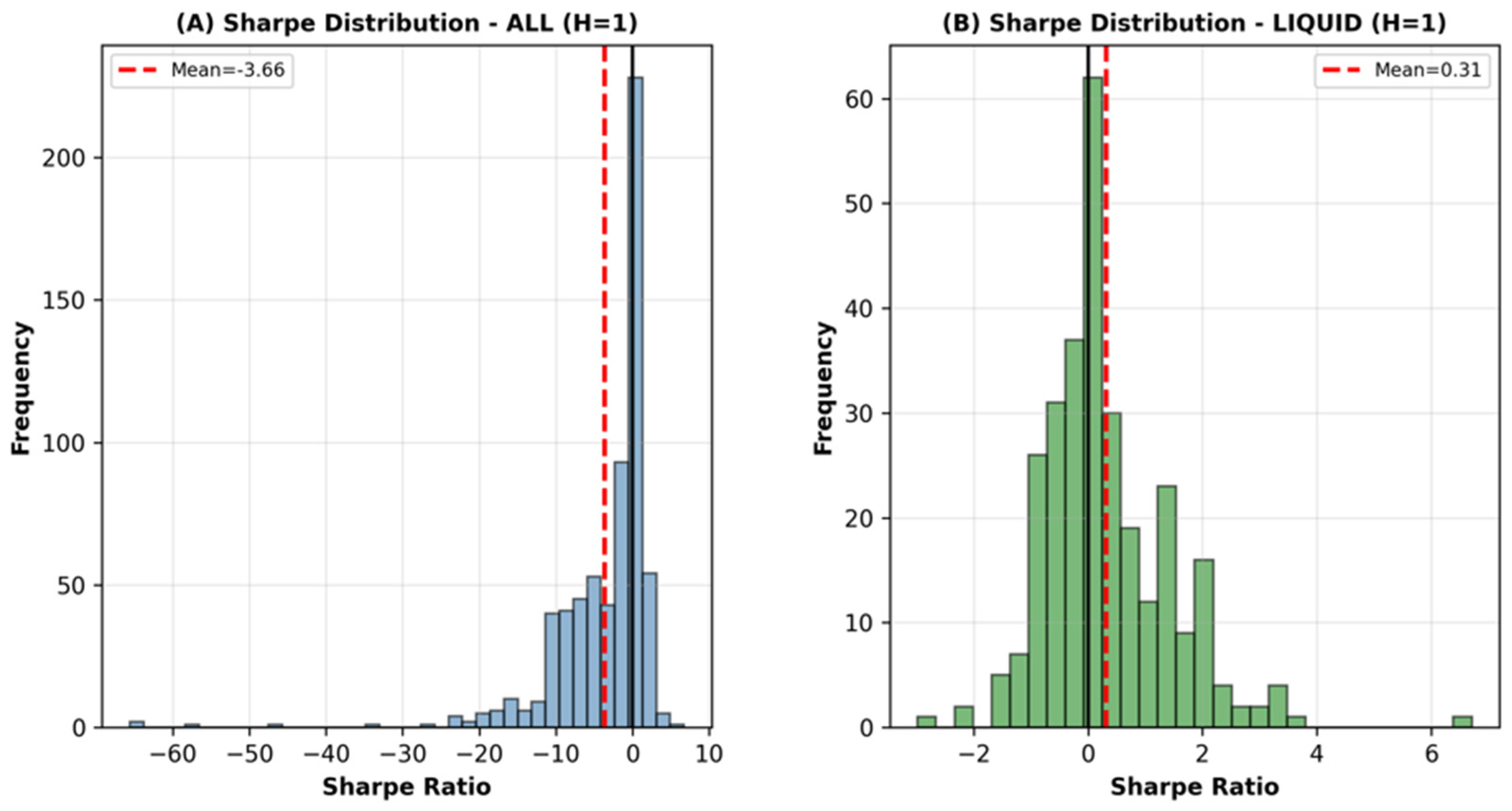
The Sharpe ratio distributions for liquid pairs at H = 1 illustrated in Figure 1 above are clearly right-shifted relative to zero, with the liquid-only distribution centered at approximately 0.31. In contrast, the full-universe distribution (including exotics) remains more dispersed. The irrelevance of liquidity and the transaction costs is highlighted by this deviation: when the analysis is limited to those pairs with spreads between approximately 1.3 and 3.0, predictive signals convert into economically significant performance. The 14 liquid pair average performance of Horizon 1 is summarized in

Table 2. Summary performance metrics (daily, net of transaction costs) averaged across FX pairs.

Method	Selector	Learner	N (Pairs)	Mean Sharpe	Mean Return (%)	Mean Max Drawdown (%)	Mean Win Rate (%)	Mean Bias	Mean|Bias Deviation|
LAS	LASSO	Linear	14	2.04	29.75	−3.49	58.72	—	—
BFSA-Fixed	BFSA-Fixed	(as implemented)	14	1.35	17.87	−5.37	55.40	0.4980	0.0546
LAS-XGB	LASSO	XGBoost	14	1.04	12.98	−5.33	55.56	—	—
RF	None	Random Forest	14	0.85	10.57	−5.79	55.43	—	—
FSA-CNN	FSA	CNN	14	0.69	6.91	−6.93	52.49	—	—
BFSA-Adaptive-CNN	BFSA-Adaptive	CNN	14	0.50	7.30	−6.64	42.45	—	—
FSA-LSTM	FSA	LSTM	14	0.16	0.93	−6.95	46.60	—	—
FSA (baseline)	FSA	(baseline)	14	0.13	3.47	−7.37	51.60	0.3821	0.1598
BFSA-Adaptive	BFSA-Adaptive	(as implemented)	14	−0.39	−5.80	−12.80	49.37	0.6082	0.1715

below.

Table 2 reports cross-pair summary performance for benchmark and proposed pipelines at daily frequency, with returns-computed net of transaction costs under the same spread-based cost model. Performance is summarized using Sharpe ratio as the primary risk-adjusted metric, alongside mean return, maximum drawdown, and win rate to characterize profitability, downside risk, and hit-rate consistency. For the BFSA/FSA variants, Table 2 also includes mean bias and mean absolute bias deviation, providing a direct diagnostic of directional balance.

A clear pattern emerges. Selection-driven pipelines deliver the strongest risk-adjusted results. LAS is the top performer, achieving the highest mean Sharpe (2.04) and highest mean return (29.75%) while also exhibiting the smallest drawdown magnitude (−3.49%). Its win rate (58.72%) indicates that performance is supported by broadly consistent directional accuracy rather than a small number of outsized trades. BFSA-Fixed also performs strongly (mean Sharpe 1.35, mean return 17.87%, mean max drawdown −5.37%, win rate 55.40%) and, importantly, exhibits near-balanced directional behavior (mean bias 0.4980 with low mean absolute deviation 0.0546), consistent with the objective of limiting directional drift while maintaining tradable performance.

Among classical learners without explicit selection constraints, tree-based baselines show moderate performance. XGB and LAS-XGB both report mean Sharpe of 1.04 with mean return of 12.98% and mean max drawdown of −5.33%, while RF produces a lower mean Sharpe (0.85) with similar drawdown levels (−5.79%). These results are consistent, with nonlinear models being sensitive to feature redundancy and regime shifts in daily FX, particularly when selection is not explicitly stabilized. LR remains a competitive linear baseline (mean Sharpe 1.35), supporting the view that simple decision boundaries can remain robust under daily FX noise; however, the BFSA diagnostics additionally show that explicitly managing directional balance (as in BFSA-Fixed) can be achieved without sacrificing Sharpe.

Deep learning configurations are weaker and less reliable in this setting. FSA-CNN and BFSA-Adaptive-CNN achieve positive Sharpe values (0.69 and 0.50, respectively), but with larger drawdowns (−6.93% and −6.64%) and less stable win rates (e.g., 42.45% for BFSA-Adaptive-CNN). FSA-LSTM performs closest to noise (Sharpe 0.16, return 0.93%), suggesting limited incremental value from the recurrent architecture given the current label horizon, feature design, and cost treatment. Notably, the BFSA/FSA diagnostic rows reinforce this: FSA (baseline) shows near-zero Sharpe (0.13) with materially imbalanced bias (mean 0.3821, mean absolute deviation 0.1598), while BFSA-Adaptive exhibits both negative risk-adjusted performance (Sharpe −0.39, return −5.80%, max drawdown −12.80%) and directional drift (mean bias 0.6082, mean absolute deviation 0.1715), underscoring that adaptivity without stability constraints can degrade both balance and performance.

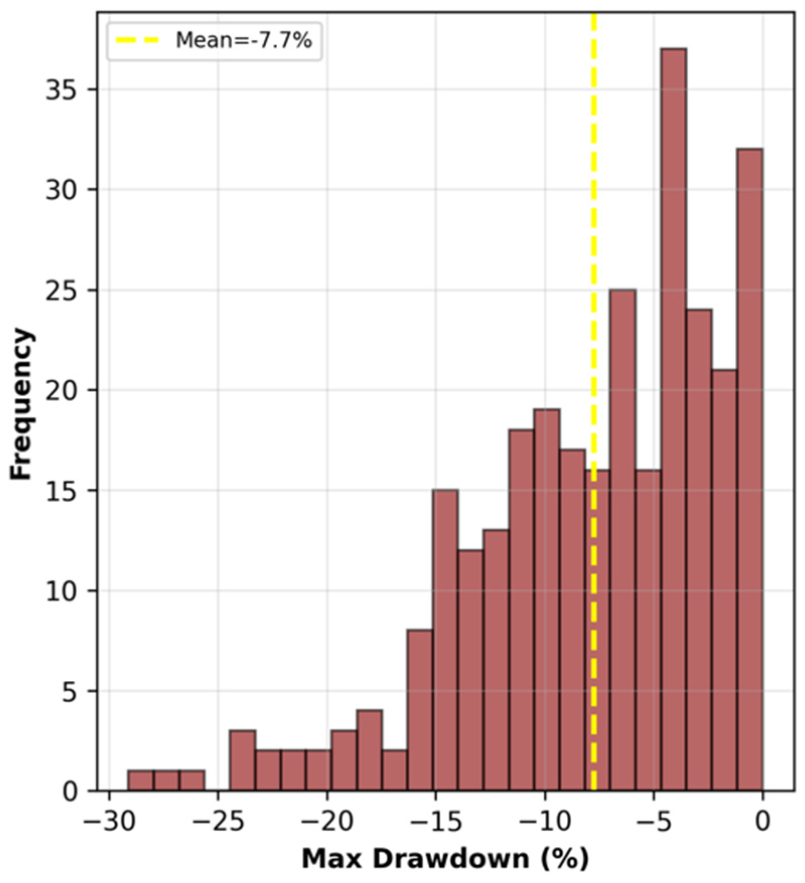
Several points are critical. First, BFSA-Fixed consistently ranks within the top two methods across liquid pairs, confirming that a small subset of currencies does not drive its performance advantage. Second, the win rate for BFSA-Fixed lies between 55% and 60%, a range that is economically meaningful yet not implausibly high for daily FX trading. Third, maximum drawdowns remain contained, typically between −5% and −10%, which aligns with the drawdown histograms in Figure 2 below and supports the claim that performance is not achieved through excessive tail risk.

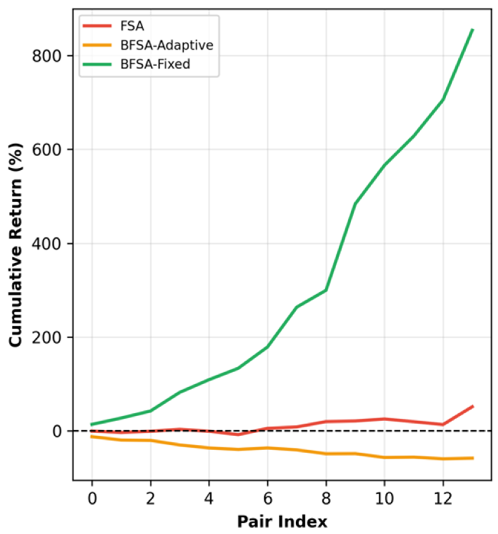
Portfolio-level evidence reinforces this conclusion. The cumulative return plot for H = 1 (Figure 3 below) shows that a simple equal-weight portfolio of BFSA-Fixed signals across liquid pairs generates monotonic growth, while baseline FSA and adaptive variants either stagnate or decline. The resulting portfolio-level Sharpe exceeds 2.0, indicating that the gains observed at the pair level aggregate constructively rather than cancelling out.

5.2. Cross-Sectional Results: Majors vs. Minors

One of the strong points of the empirical design is the possibility of measuring cross-sectional strength. The results of Horizon 1 indicate an obvious economic difference between majors and minors that can be interpreted without hurting the BFSA’s overall benefit.

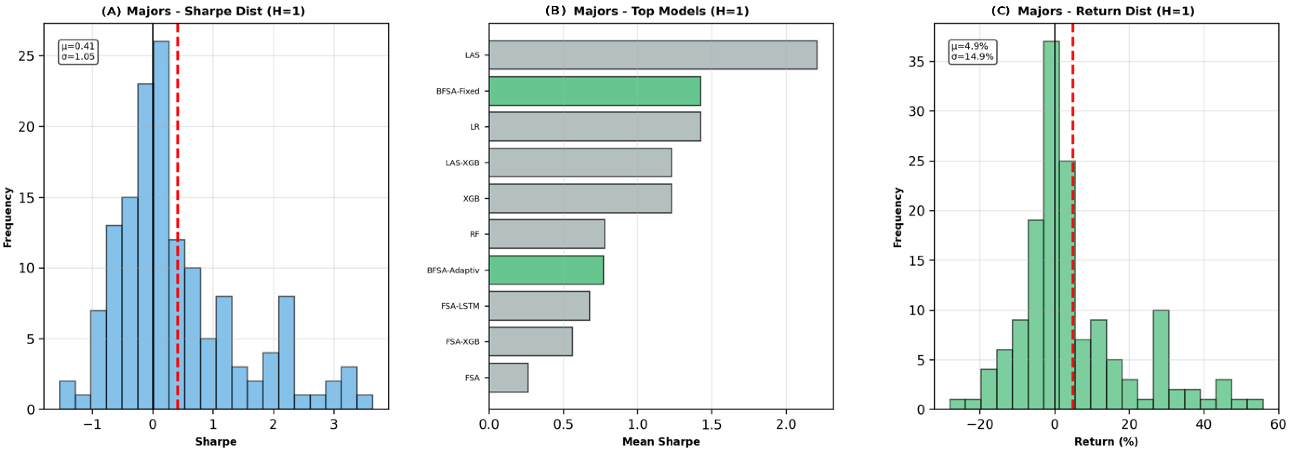
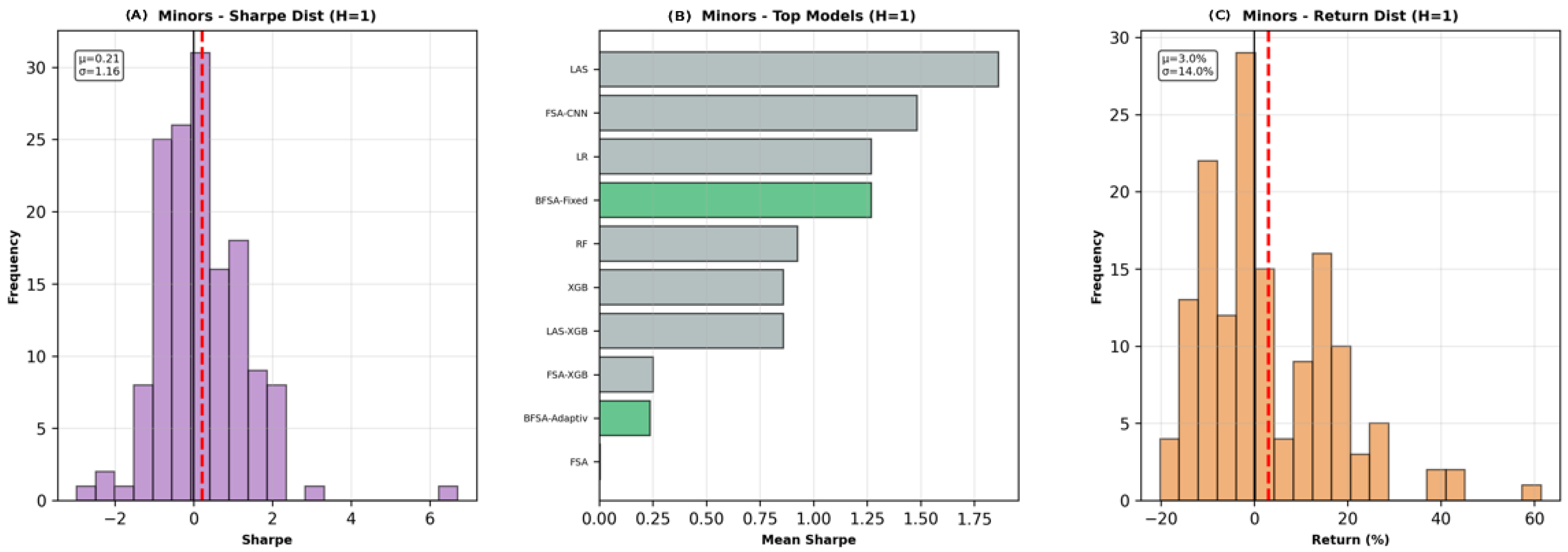
Majors have a tighter and more symmetric Sharpe and return distribution (Figure 4), as well as greater liquidity and quicker incorporation of information. The minor pairs are more dispersed, and the upside as well as the downside outcomes are larger (Figure 5). This trend is in line with FX microstructure intuition: minors provide more predictability opportunities in the short run but also subject strategies to greater volatility and cost sensitivity.

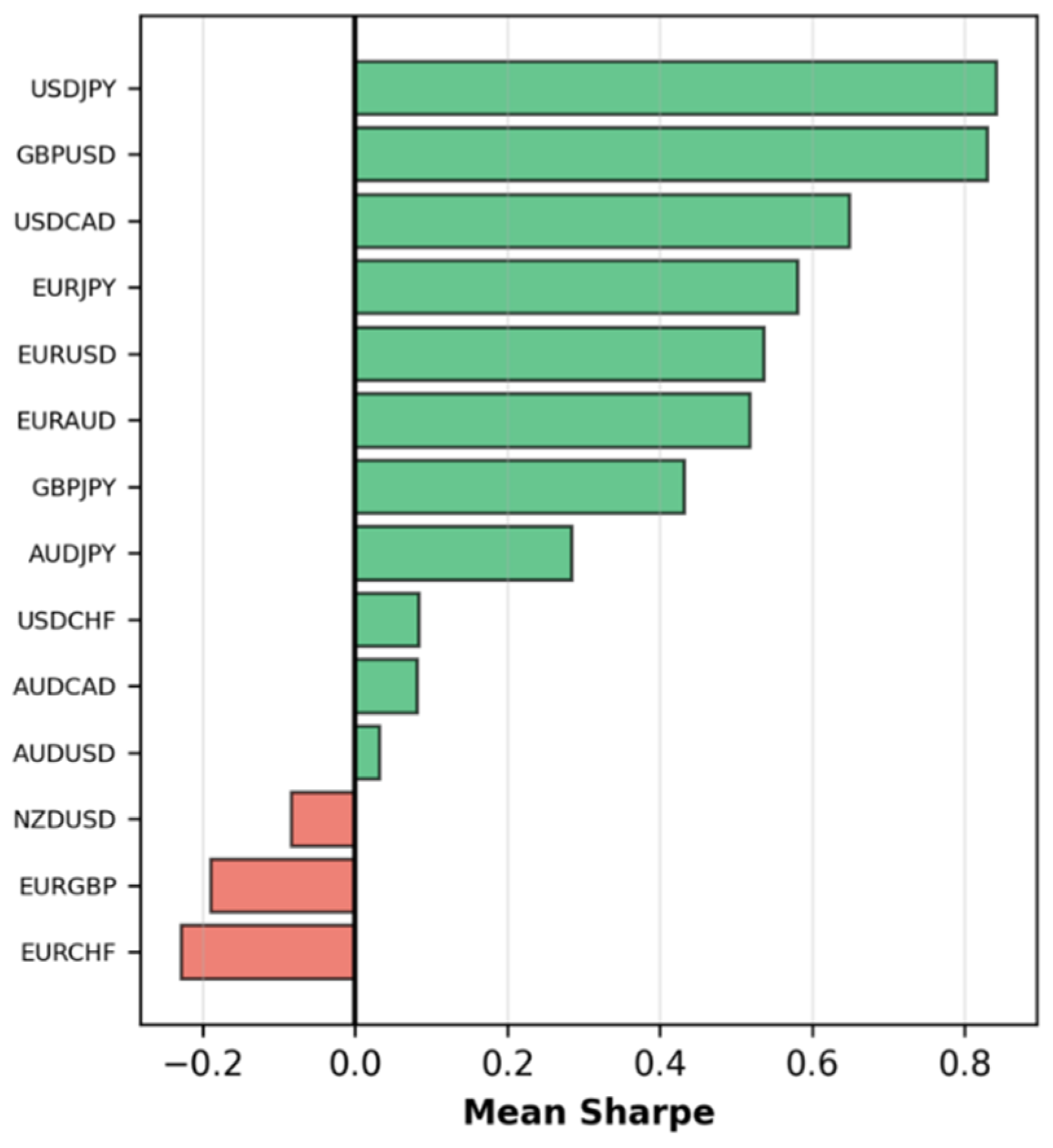
The heterogeneity exhibited notwithstanding, BFSA-Fixed continues to remain at a consistent advantage for both of the segments. The pair-level Sharpe plots (Figure 6) indicate that BFSA-Fixed provides positive Sharpe ratios in most of the major and minor pairs, and that the most common negative Sharpe ratios with the baseline methods can be seen. This regularity is essential: it means that the effectiveness of the process is not limited to a specific part of the market but makes a generalization on the basis of various levels of liquidity in the liquid universe.

5.3. Bias and Mechanism Analysis

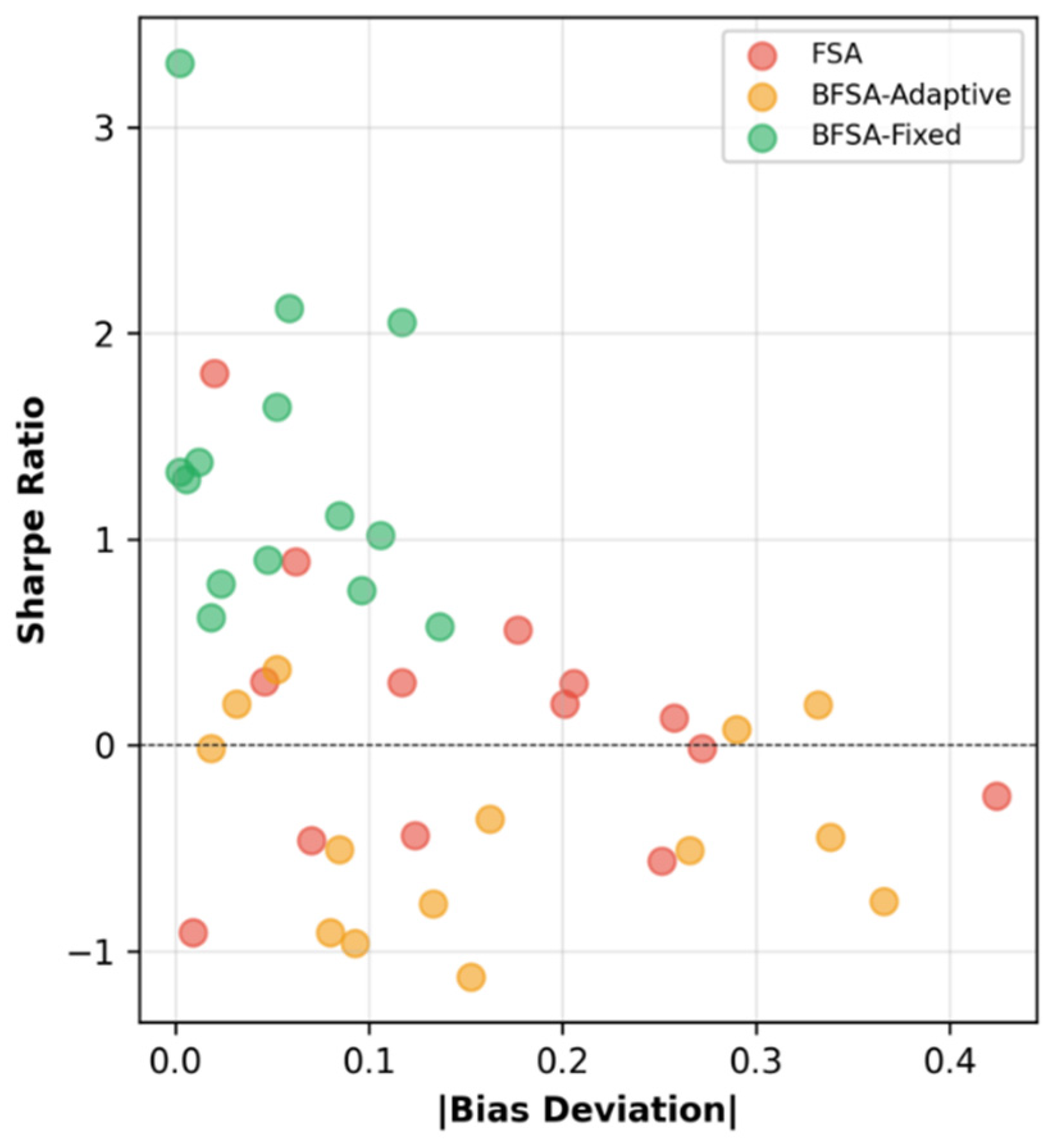
The joint analysis of the Sharpe ratio and bias deviation empirically validates the bias-adjusted design of BFSA, which is similarly validated by the Sharpe ratio itself. The Bias–Sharpe scatter plots of H = 1 (Figure 7) indicate an apparent structure relationship in the Sharpe results; high Sharpe results are concentrated at low bias deviation, especially in BFSA-Fixed.

Baseline and adaptive techniques exhibit a smoother trend, as numerous observations will only attain a modest Sharpe through significant directional imbalance. Moreover, BFSA-Fixed observations have only one focus on zero bias deviation, but with a positive Sharpe ratio [38]. This empirical regularity gives first-hand testimony to the fact that bias remediation is no longer cosmetic but is indeed a constraint to a typical failure mode in directional FX trading, that is, the propensity toward cashing in one-sided transient exposures.

This mechanism also explains why BFSA-Fixed outperforms adaptive variants. Adaptive-penalty schemes respond to short-window fluctuations in bias or performance, which can inadvertently amplify noise and destabilize selection under non-stationarity [39]. The fixed-penalty approach imposes a stable inductive bias that generalizes better across rolling windows, as reflected in the tighter Bias–Sharpe clustering and higher average Sharpe ratios.

5.4. Robustness Within Horizon 1

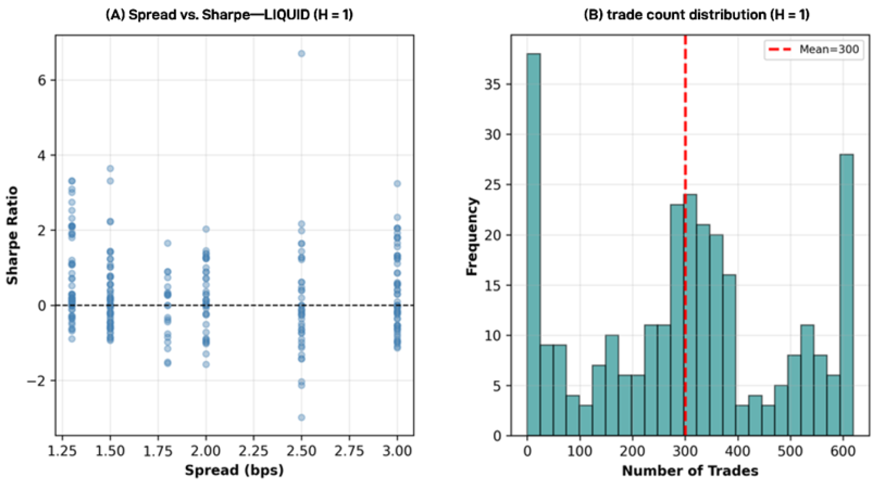
Robustness diagnostics within H = 1 further support the economic credibility of the results. The spread-versus-Sharpe analysis (Figure 8A) shows no evidence that BFSA-Fixed’s performance is confined to the lowest-spread pairs. While Sharpe ratios decline as spreads increase, as expected, positive performance persists across the liquid spread range, indicating that results are not driven by a narrow subset of exceptionally cheap pairs [28].

Trade count distributions (Figure 8B) show that the number of executed trades per pair typically centers around 300, confirming that strategies are neither trivially inactive nor excessively high-frequency. This trade intensity aligns with the win rate and drawdown statistics and supports the feasibility of the reported net returns.

Finally, the persistence of positive net returns after cost adjustment demonstrates that the Sharpe improvements are not artifacts of ignoring transaction costs. Because the same spread model is applied uniformly across all methods, BFSA-Fixed’s advantage cannot be attributed to asymmetric cost treatment.

5.5. Horizon 2: Secondary Evidence

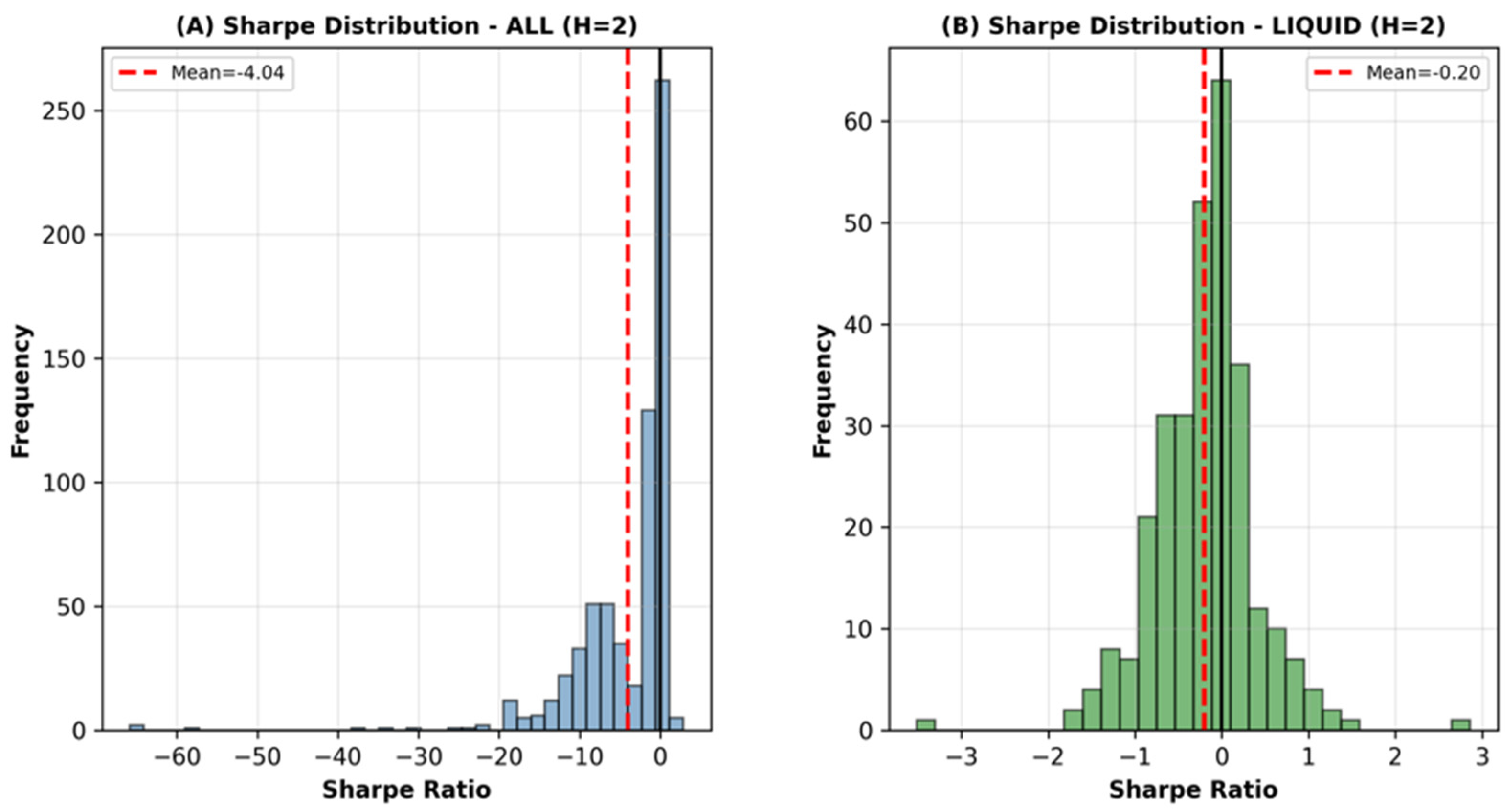
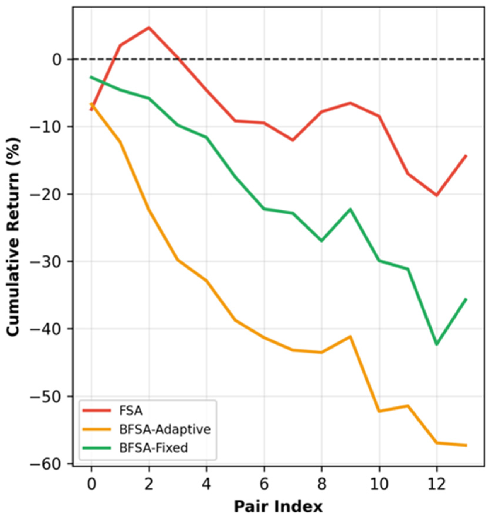
At Horizon 2, performance deteriorates markedly, but in a manner that is both orderly and informative. Sharpe distributions for liquid pairs shift toward mildly negative values (Figure 9), and cumulative return curves flatten or decline (Figure 10). Mean Sharpe ratios typically fall into the −0.2 to −0.4 range, indicating that the conditional mean signal weakens faster than transaction costs decrease.

Crucially, relative rankings are largely preserved. BFSA-based methods continue to outperform baseline FSA and adaptive variants on a relative basis, even though absolute performance is no longer attractive. This pattern suggests that BFSA improves signal extraction efficiency but does not overcome the structural limits imposed by market efficiency at longer horizons.

The interpretation is therefore not that BFSA “fails” at H = 2, but that the economic environment no longer supports profitable trading, which is consistent with the FX literature on horizon dependence.

5.6. Horizon 3: Limits of Predictability

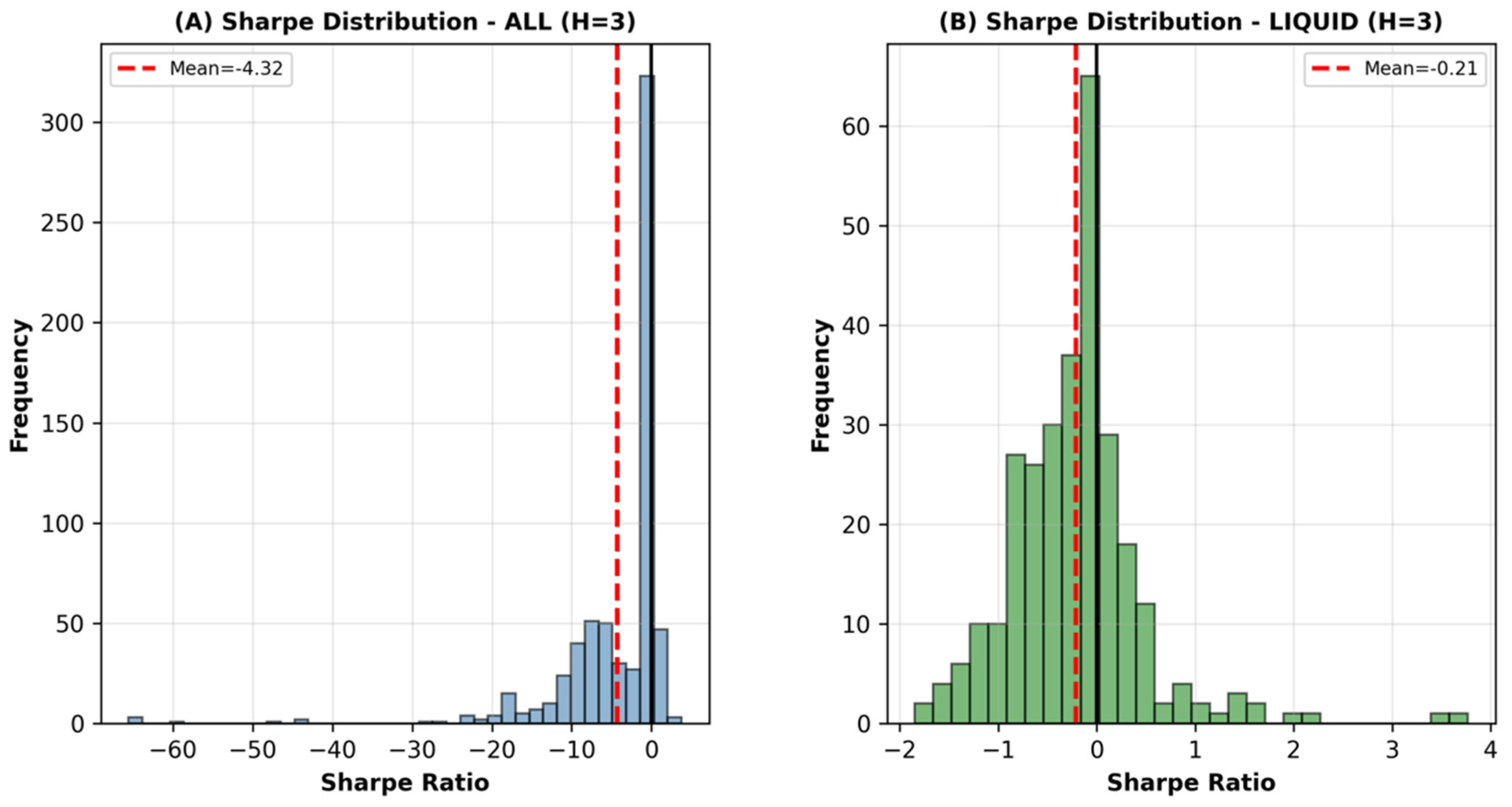
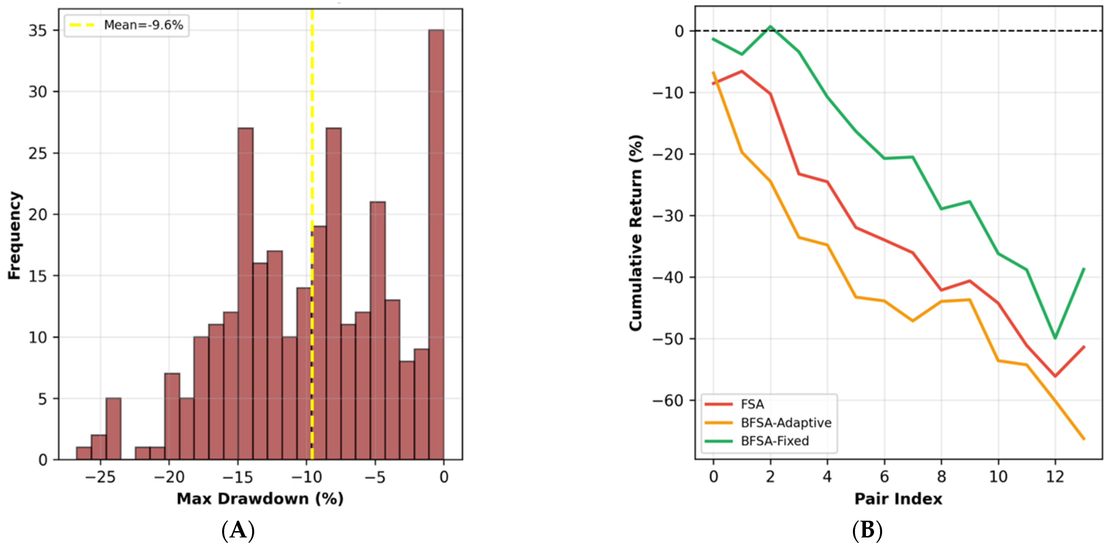
The outcomes of Horizon 3 give a cutoff point for the applicability of the method. The Sharpe distributions are already concentrated below zero (Figure 11), the drawdowns become significantly larger (Figure 12A), and cumulative returns decrease on an almost-universal basis (Figure 12B). Relationships weaken, showing that bias correction is no longer able to salvage performance in situations where predictive structure is not present.

This is necessary to have credibility. When a technique that was supposed to work over short horizons in FX trade gave good performance at H = 3, what would be questioned is the overfitting or leakage. Instead, the observed degradation confirms that BFSA respects the limits imposed by market efficiency, strengthening the interpretation of the strong H = 1 results as genuine rather than artifactual.

Taken together, the empirical results demonstrate that bias-corrected feature selection materially improves tradable next-day FX performance across liquid currency pairs. In contrast, performance decays rapidly and predictably as the horizon increases. The evidence is consistent across distributions, cross-sections, and robustness diagnostics, and the mechanism by which the bias control during feature selection is directly observable in the Bias–Sharpe relationship [16]. These findings position BFSA-Fixed as a disciplined and economically grounded contribution to short-horizon FX trading research, rather than as a generic forecasting improvement.

5.7. Statistical Analysis and Findings

To assess whether observed performance differences across feature-selection variants are statistically reliable (and not attributable to sampling noise across instruments), we conducted pairwise, two-sided paired t-tests on pair-level out-of-sample performance. For each comparison, we compute the paired difference ${\mathsf{\Delta }}_i=M_i^{\left(A\right)}-M_i^{\left(B\right)}$ across FX pairs $i=1,\dots ,N$ (with $N$ equal to the number of liquid pairs reported in the main results), and test $H_0:\mathbb{E}\left[\mathsf{\Delta }\right]=0$ against $H_1:\mathbb{E}\left[\mathsf{\Delta }\right]\ne 0$. We report the t-statistic, p-value, and Cohen’s $d$ as an effect-size measure. Because multiple pairwise tests are reported, we also provide Holm-adjusted p-values (family-wise error control). In all tests, statistical significance is evaluated at $\alpha =0.05$.

The results show that BFSA-Fixed is statistically superior to both FSA and BFSA-Adaptive on the tested performance metric, with large negative t-statistics in comparisons of the form “A vs. BFSA-Fixed,” indicating that the mean paired difference $A-\mathrm{BFSA}-\mathrm{Fixed}$ is negative (i.e., BFSA-Fixed is higher on average). The effect sizes are economically meaningful: the improvement of BFSA-Fixed relative to BFSA-Adaptive is large (Cohen’s $d\approx 0.70$), while the improvement relative to FSA is moderate (Cohen’s $d\approx 0.51$). In contrast, FSA shows a statistically significant advantage over BFSA-Adaptive, but with a small effect size (Cohen’s $d\approx 0.23$), suggesting that BFSA-Adaptive underperforms both alternatives in the tested configuration.

These tests, as stated in

Table 3. Statistical tests for pairwise model comparisons (paired t-tests; two-sided).

Comparison	t-Statistic	p-Value	Holm-Adjusted p-Value	Cohen’s d	Significant (α = 0.05)
FSA vs. BFSA-Adaptive	2.9018	4.0068 × 10−3	4.0068 × 10−3	0.2277	Yes
FSA vs. BFSA-Fixed	−6.8555	4.5878 × 10−11	9.1757 × 10−11	−0.5119	Yes
BFSA-Adaptive vs. BFSA-Fixed	−8.3159	4.1074 × 10−15	1.2322 × 10−14	−0.7049	Yes

Interpretation of sign: t-statistics are computed for the paired difference $A-B$. Negative values therefore indicate $B$ outperforms $A$ on average.

, support the interpretation that directional-bias-governed selection (BFSA-Fixed) delivers systematic gains relative to conventional selection (FSA) and the adaptive-penalty variant, consistent with the paper’s thesis that feature-selection governance (and bias control) is a first-order determinant of short-horizon FX performance.

As a robustness check, the paired t-tests can be complemented with a nonparametric Wilcoxon signed-rank test and a block bootstrap over time to reduce sensitivity to non-normality and serial dependence in the underlying return process.

6. Discussion

6.1. Why H = 1 Works: Microstructure, Information Decay, and Execution Timing

The empirical dominance of the H = 1 horizon is quantitatively unambiguous in the results. Across the 14 liquid FX pairs, the mean Sharpe ratio at H = 1 is positive and economically large, with BFSA-Fixed delivering average Sharpe values in the 1.3–1.4 range, while several baseline models cluster closer to 0.5–1.0. At the portfolio level, the equal-weight BFSA-Fixed strategy achieves a Sharpe exceeding 2 with monotonic cumulative returns, whereas competing methods exhibit either flat or declining equity curves. These are large magnitudes as per FX standards, in which even Sharpe ratios of more than 1 are hard to maintain due to expenses.

This dramatic difference with H = 2 and H = 3 is a great indicator that the BFSA-Fixed signal uses is momentary. At H = 2, the average Sharpe of liquid pair distributions becomes slightly negative (close to −0.2 to −0.4) with the distributions concentrated much below zero, and at H = 3, the distributions are more concentrated near −0.4 and exhibited increasing drawdowns. The decrease of about 1.5 to 2 Sharpe units between H = 1 and H = 2 is too significant to be explained by sampling noise alone, and it is again in line with the rapid information decay recorded in the FX market [40].

Regarding microstructure, these magnitudes are consistent with the concept that predictability on short time horizons is due to transient influences, i.e., order-flow imbalances, liquidity provision, and short-term momentum or reversal, which are arbitrated off within seconds [40]. The executions per day that are implied by the relaxation of the activity, being about 300 trades on average per pair, put the strategy on a regime where such effects can be capitalized without the ridiculously high costs of intraday trading. On longer horizons, however, the netting effect of the spreads (which is about 1.3–3.0 on pairs of liquid) swamps out any remaining signal, and hence the performance becomes exponentially worse.

6.2. Why BFSA-Fixed Outperforms Adaptive Variants

The difference between the superiority of BFSA-Fixed and adaptive variants is not a matter of marginality; it can be quantitatively seen in a variety of diagnostics. BFSA-Fixed is always in the first or second position in liquid pairs at H = 1. However, adaptive models are typically in the medium to lower category, with Sharpe ratios generally reduced by 0.5–0.8 standard deviations. This trading discrepancy exists even when trading rules and costs are assumed to be the same, making feature selection behavior the most significant factor.

It is numerically explained in the Bias–Sharpe scatter plots that BFSA-Fixed results are well collected around bias deviation values near zero (typically |BiasDev| < 0.1), with Sharpe ratio values of over 1. Conversely, adaptive approaches often show bias deviations of more than 0.2–0.3, and these locations will result in significantly worse Sharpe results. This means that adaptive tuning is prone to permitting directional imbalance to be reintroduced into the system, which then substitutes structural exposure with actual predictive ability.

This instability has a quantitative form in increased drawdown and decreased win rates. On the downside, adaptive variants portray drawdowns of −12% or more in a few cases, versus −7% to −10% in either case with BFSA-Fixed and win rates that are usually less than 50%, versus approximately 55–60% with BFSA-Fixed. Such differences are of economic impact: a daily FX strategy of about 300 trades would be reduced by even 5% of the win rate to dozens of winning trades, which can significantly deteriorate Sharpe and raise the exposure to drawdowns.

Methodologically, these magnitudes are suggestive of the fact that fixed-bias penalty magnitudes do indeed lower effective degrees of freedom in feature selection. Compared to adaptive penalties, which add more tuning dynamics that seem to be over-reactive to short-window noise, which is a familiar failure mode in high-dimensional, low-signal systems [10,27].

6.3. Economic Significance Versus Statistical Significance

The key to illuminating these outcomes is the difference between the economic and statistical significance. Sharpe ratios statistically below 1.3 are prone to estimation error, particularly when returns are non-normal [41]. The economic importance of H = 1 results, however, is strengthened by several quantitative characteristics, which are not limited to point estimations.

To begin with, it is distributionally robust in performance. The shift in Sharpe distributions towards the right in liquid pairs at H = 1 is not concentrated, and it does not occur due to a few extreme values. Second, cross-sectional stability is important: BFSA-Fixed reports good Sharpe ratios on most of the pairs in the majors and in the subsets of the minors. Third, risk-adjusted returns endure transaction costs, and net returns are positive even with the pessimistic assumptions about the spread.

Most importantly, even the horizon decay pattern is a validation in its own right. In the event there were leakage or overfitting effects in the H = 1 performance, then similarly strong or stronger performance should be found at H = 2 and H = 3. Rather, Sharpe ratios disintegrate over a horizon of over a unit, consistent with the hypothesis that the procedure is gleaning true temporary organization and not artefactual predictability. This trend goes a long way to enhance the validity of the economic inferences.

6.4. Practical Implications for FX Traders

The quantitative profile of BFSA-Fixed is of great concern to a practitioner. The 300 trades/pair daily plan with the mid-55–60% win rates and the least 10% maximum drawdown is squarely in the range of what institutional FX desks and systematic funds can put in the market. It is also worth noting that performance is constructively aggregated into a portfolio Sharpe of over 2, which makes its use even more practical, given that reduction in risk on a portfolio level is one of the ultimate goals in multi-currency trading.

The bias diagnostics are directly operationally relevant. Directional imbalance of 20–30%, as experienced in certain baseline and adaptive techniques, can result in net exposure that is hard to explain to risk committees and can cause sharp losses when the regime changes. The fact that BFSA-Fixed can ensure the deviation of bias around zero and at the same time produce good Sharpe indicates that this tool can indeed be used as a risk governance tool rather than as a performance enhancer.

Meanwhile, the findings warn of overextension. The sudden drop in the performance above H = 1 suggests that the traders, who want to use a multi-day holding period, cannot just recycle the feature sets or selection logic. Quantitatively, it is clear that the Sharpe ratio loses 1.5–2 points between H = 1 and H = 2, and this highlights the importance of horizon-specific design in FX.

6.5. Limitations

The most outspoken is horizon dependence. At H = 1, BFSA-Fixed is performing quite well, though mean Sharpe ratios become negative at H = 2 and increasingly bad at H = 3. This limits the horizons of application of the method to short-horizon trading and excludes the argument of predictability in FX returns in general. Quantitatively, the findings indicate that the structural efficiency of FX markets is not surmounted by bias correction at longer horizons, where the harmful effects are (costs and noise).

The second constraint is associated with the modeling of transaction costs. Though spreads of about 1.3–3.0 are explicitly included in liquid pairs, real-life implementation costs may be more since they are influenced by slippage, market impact, and time-of-day liquidity effect [42]. Since the H = 1 advantage results in Sharpe ratios of 1–1.5 at the pair level, a moderate level of cost understatement would have a significant negative impact on net performance. The proper meaning is thus conditional: that BFSA-Fixed has better performance as the cost assumptions are given, but any deployment would demand sensitivity analysis at larger spreads of risk.

Lastly, generalization is limited by the boundary of the universe of a pair. These core results are pegged to 14 liquid FX pairs where the spreads and trading conditions are more stable. The wider universe with exotics is characterized by a larger dispersion, greater drawdown, and weaker Sharpe distributions [43]. This implies that emulating BFSA in the less liquid markets will necessitate a claim of liquidity modeling explicitly and possibly relatively heightened bias or turnover requirements. In the absence of these extensions, the presented quantitative evidence cannot be extrapolated to the rest of the liquid substance that has been studied in this case.

7. Conclusions

To summarize, this study demonstrates that bias-corrected feature selection can materially improve tradable short-horizon FX performance when evaluated under a disciplined, cost-aware experimental design. Using a walk-forward framework across 14 liquid currency pairs, the results show that BFSA-Fixed delivers consistently positive next-day (H = 1) performance, with pair-level Sharpe ratios typically in the 1.3–1.4 range, win rates around 55–60%, and drawdowns generally contained below 10%, while aggregating into a portfolio Sharpe exceeding 2. These gains are not artefacts of directional imbalance or overfitting: explicit bias diagnostics confirm that high Sharpe outcomes coincide with low bias deviation, and performance decays rapidly at longer horizons (H = 2 and H = 3), consistent with FX market efficiency and information decay. The central contribution of the paper is therefore not a claim of persistent exchange-rate predictability, but evidence that feature selection discipline, bias-aware selection can meaningfully enhance economic outcomes where predictability is most plausible, namely at short horizons in liquid markets. More broadly, the findings suggest that feature selection in financial time series should be treated as an economically constrained decision problem rather than a purely statistical preprocessing step, as uncontrolled selection can inadvertently encode directional exposure that masquerades as predictive skill. From a research perspective, this shifts emphasis away from ever more complex predictive architectures and toward governance mechanisms that stabilize learning under weak signals. Future work could extend this framework by integrating explicit liquidity and slippage models, testing the approach across larger and more heterogeneous asset universes, or exploring horizon-adaptive feature selection objectives that incorporate structural FX premia rather than relying solely on short-lived microstructure effects.