WM-Classroom v1.0: A Didactic Multi-Species Agent-Based Model to Explore Predator–Prey–Harvest Dynamics

Simple Summary

Wildlife populations and people interact in complex ways. Managers must decide how many individuals of which species can be taken, how many hunters are active, how long the season lasts, and whether predators can be legally removed. We built WM-Classroom v1.0, a simple, teaching-oriented computer model that lets students and trainees explore how these decisions can change the behavior of a simplified wildlife community with a predator, two prey types, and human harvesters. The model runs on a small grid “landscape” and follows weekly steps of movement, feeding, and (when allowed) hunting. By turning rules on and off—such as season length, minimum population cut-offs for harvest, numbers of hunters, and predator control—users can immediately see how prey and predator numbers rise and fall over time. As such, it helps learners connect simple rules to emerging patterns, understand trade-offs, and practice “what-if” experiments in a transparent, open way. Although the current version of the tool is not meant to predict actual numbers in real-world communities, it can be used in high-school and undergraduate ecology classes, training for wildlife surveyors and officers, selective cull-hunter education, citizen seminars, and decision-maker workshops, with the potential to be further developed and tailored to specific case studies.

Abstract

We present WM-Classroom v1.0, a pedagogical multi-species agent-based model (ABM) designed for educational purposes in predator–prey–harvest systems. The model embeds a predator, two prey breeds, and human harvesters on a homogeneous 50 × 50 grid with weekly time steps, implementing random movement, abstract energetics, prey consumption, reproduction, legal harvest with species-specific cut-offs and seasons, optional predator control, and a poaching switch. After basic technical checks (energetic calibration, prey composition, herbivore viability), we explore the consistency of the model under illustrative scenarios including no hunting, single-prey harvest, hunter-density and season-length gradients, predator removal, and poaching. In the no-hunting baseline (n = 100), mean end-of-run abundances were 22 deer, 159 boar, and 45 wolves, with limited extinction events. Deer-only harvest often drove deer to very low end-of-run counts (mean 1–16) with extinctions in 2–7/10 replicates across cut-offs, whereas boar-only harvest showed higher persistence (mean 11–74) and boar extinctions occurred only at the lowest cut-off (3/10). Increasing hunter numbers or season length depressed prey and could indirectly reduce wolves via prey depletion. Legal predator control reduced predators as designed, while poaching had little effect under the implemented rules. Because interaction and prey-choice rules are simplified for transparency, outcomes should be interpreted as conditional on model assumptions. WM-Classroom v1.0 provides a didactic sandbox for courses, professional training, and outreach, with extensions (habitat heterogeneity, age/sex structure, probabilistic diet/kill success, and calibration/validation) outlined for future versions.

1. Introduction

Over the last decades, European wildlife populations have undergone intense demographic shifts [1]. Wild ungulate populations have rebounded, especially red deer (Cervus elaphus) and wild boar (Sus scrofa) that have expanded substantially [2,3]. At the continental scale, reported red deer spring abundance increased from ~1.1 to ~1.7 million between 1984 and the early 2000s, with hunting bags rising from ~275,000 to ~429,000 individuals [4]. Similarly, across 18 European countries, wild boar hunting bags increased from ~864,000 (1992) to >2.2 million (2012) [5]. Meanwhile, large carnivores and medium-sized canids, including gray wolves (Canis lupus) [6,7,8,9,10,11], Eurasian lynx (Lynx lynx) [12,13,14], golden jackal (Canis aureus) [13], and brown bear (Ursus arctos) [15,16], have recolonized or extended their ranges. The most recent continental update estimates ~23,000 wolves in Europe in 2023 (≈35% increase since 2016), around 20,500 brown bears, ~9000 Eurasian lynx, and >150,000 golden jackals, confirming a broad recovery trend with clear implications for ecosystem management in human-dominated landscapes [2,6,17,18]. Managers therefore face a moving target: high densities of ungulates and other browsing/grazing species can cause crop damage, vehicle collisions, and forest regeneration issues, while large predators tend to trigger conflicts with livestock production, game management, and public perception [2,6,19].

These long-term trends create complex management challenges involving human and wildlife coexistence, sustainable harvest, and predator–prey dynamics [3,20,21,22]. Census, monitoring effort, as well as hunting policy play a central role in this context. Decisions about which species may be harvested, how many hunters are active, how long the hunting season lasts, and whether predator control is permitted are commonly revisited; additionally, the reality that illegal take can occur, even if usually at low rates, complicate the dynamics in some systems even more [23,24,25,26]. Selective harvest has well-known demographic and behavioral side-effects, namely biasing sex ratios, truncating age structure, slowing body-mass development, shifting offspring sex ratios, disrupting social hierarchies, and altering space use and activity patterns [5,24,25].

These class- and behavior-mediated processes have long been explored with classic modeling approaches, including mathematical approaches based on Lotka–Volterra equation systems [27,28] and matrix models [29], which have provided valuable insights [30]. Yet, they typically represent populations at aggregate levels, which makes it difficult to encode individual variability, movement ecology, individual-level interactions such as prey choice and predator–prey encounter likelihood, as well as rule-based human behavior (e.g., harvest cut-offs or season closures).

Given these limitations, quantitative insights can be generated through two complementary approaches. Data-driven studies (e.g., statistical or mechanistic population models calibrated and validated against empirical monitoring data) aim to estimate parameters, reconstruct dynamics, or support forecasting in specific systems [31]. By contrast, computer-simulation approaches such as agent-based models (ABMs) represent individuals and their interactions explicitly and are often used to explore how simple rules can generate emergent patterns under alternative assumptions or management scenarios [32]. ABMs are especially well-suited for exploring how individual behavior and local interactions scale up to system-level outcomes, because they simulate organism-based processes and adaptations to local biotic and abiotic conditions, allowing the effects of environmental change to propagate from individuals to communities and even ecosystems. ABMs are routinely used to study how abiotic drivers, shifting biotic interactions, and their combinations shape the spatiotemporal distribution of organisms [33]. As such, ABMs offer a promising way to explore complex, dynamic ecological systems [34,35]. They not only contribute to a deeper understanding of population-level dynamics, but can also allow us to investigate how individual variability, heterogeneous interactions among agents, and spatially distributed environmental resources shape community-level outcomes across different scenarios [35]. Moreover, ABMs can be more easily integrated with Geographic Information Systems (GIS) which provide geographic, topographic and environmental variables in a spatialized framework (2D or 3D). This integration makes it possible to represent the landscape and ecological features of the study area that are regarded as most crucial in shaping both wildlife and human choices [36].

By representing animals and humans as interacting agents embedded on a landscape, ABMs have the potential to support the visualization and the exploration of management levers in terms of what species may be harvested, when, under which conditions, and with what expected feedback [32,37,38,39].

Under this perspective, the ABM framework is especially valuable for teaching and exploratory purposes, where transparency, inspectability, and the ability to “trace” emergent patterns back to simple rules are more important than predictive performance.

In wildlife education, the most widely used pedagogical model is currently represented by the Wolf–Sheep example, distributed with NetLogo [40]. This model introduces students to stochastic movement, prey consumption, predator dynamics, and resource regrowth in a minimal system. However, this model remains intentionally simplistic: it includes only one predator and one prey, no human activity, no multi-prey diet choice, and extremely abstract representations of ecology, since its purpose is to make evident the emergence of prey–predator dynamics in an ideal case where Lotka–Volterra equations can be applied. Related NetLogo teaching models have coupled predator–prey dynamics with hunting and poaching; for example, a community model that contrasts high-fecundity ‘boars’ with protected ‘wolves’ and introduces hunters, poachers, traps, and wardens [41]. While excellent for teaching the concept of emergent trophic cycles, these models provide only limited insight into real-world management questions.

To help bridge this gap and provide a flexible teaching tool, suitable for both wildlife-management practitioners training and theoretical courses, we present WM-Classroom v1.0, an expanded and fully documented ABM designed for instructional use. WM-Classroom v1.0 extends the classic Wolf–Sheep paradigm to a European multi-prey, human-managed context, enabling learners to explore harvest cut-offs, seasonality, predator control, and poaching within a transparent and reproducible framework.

The first version of the model introduces four key modular characteristics:

(i)

A community with two preys (deer and wild boar), with distinct reproduction rates, creating asymmetric bottom-up dynamics;

(ii)

A real predator, the wolf, with documented preferences for wild boar, aligning with empirical European dietary studies;

(iii)

The presence of human hunters following explicit rules, representing legal harvest, seasonality, regulatory cut-offs, wolf control, and low-rate poaching likelihood;

(iv)

A modular rule structure, enabling users or students to activate or deactivate management mechanisms, tailor them with changes and implementation, and inspect the consequences.

The purpose of this model is didactic and exploratory: to illustrate how simple, rule-based processes can generate non-linear system-level responses, and how harvest policies can interact with predator–prey feedback in a stylized European context. The model is not intended to predict real population sizes or to provide region-specific recommendations. Instead, it functions as an exploratory scaffold—similar to a sandbox—that allows wildlife students, early-career ecologists, and policy trainees to manipulate transparent assumptions about individual behavior, interactions, and harvest rules, and to observe emergent consequences in a controlled, fully documented environment. Accordingly, the results presented here should be interpreted as illustrative dynamics conditional on the model assumptions, supporting training in scenario thinking and model interpretation rather than real-world inference.

In this paper, we present the model using a simplified ODD structure [42,43], present the workflow implemented to verify internal consistency via structural tests, report the results of exploratory test on how canonical management levers propagate through the theoretical multi-species system, and propose a roadmap for expanding the model into more realistic ecological or applied decision-support tools.

2. Materials and Methods

2.1. Purpose of the Model

We developed an ABM in NetLogo 6.3.0 to explore trophic interactions among two prey species (represented by red deer—Cervus elaphus and wild boar—Sus scrofa), one predator species (represented by the gray wolf—Canis lupus), as well as with human hunters, in a simplified, closed landscape. The model simulates weekly cycles of movement, foraging, predation, and hunting effort, allowing us to examine how variations in hunting pressure, season length, and regulatory thresholds affect multi-species dynamics. The final aim is to explore how common management levers in terms of harvest permissions by species (deer, boar, wolf), hunter numbers, season length, wolf control/poaching, and cut-off thresholds might affect multi-species dynamics on a generic European landscape.

The model targets qualitative insight and reproducibility rather than site-specific and policy-specific prediction; the environment is therefore intentionally homogeneous and does not include habitat structure, barriers, or migration processes. All vegetation is treated as a single generic food resource with uniform regrowth time, so the resulting landscape is homogeneous, and no age- or sex-specific harvest regulations are considered. These simplifications intentionally reduce ecological complexity to focus on the interactions between hunting pressure and trophic dynamics. In this way, the effects of harvest and predator–prey feedback can be isolated without confounding spatial heterogeneity.

By making the full code openly available, alongside the BehaviorSpace settings and the full documentation, we aim to offer an accessible and flexible platform for teaching and experimentation, bridging the gap between introductory ABM demonstrations and management-oriented ecological modeling.

2.2. Entities, State Variables, Processes

The model contains four agent types: deer, boar, wolves, and hunters. Each agent type carries species-specific traits such as energy, age, and reproduction probability. Hunters additionally hold a “satisfaction” variable, which modulates their motivation to hunt across weeks. The landscape consists of a toroidal grid of resource patches that alternate between grazable (food available) and depleted states according to a simple regrowth cycle.

Species-level attributes (lifespan, reproduction rates, diet preferences) were informed by the literature on Central and Southern European populations [19,44,45,46].

Simulations run at a weekly temporal resolution. In each tick, animals perform the actions and trigger processes as detailed in

Table 1. Core agent processes, rationale, and simplifications in WM-Classroom v1.0. Numeric baseline parameters and sources are reported in Supplementary Table S1.

Process	Rule (Model Implementation)	Rationale/ Empirical Basis	Model Simplification
Movement	Individuals execute a random walk: random turn + 1 patch forward each tick.	Captures basic mobility and encounter-driven interactions without specifying habitat preferences.	No habitat heterogeneity; no movement costs beyond the fixed energy loss; no species-specific movement rules.
Energy dynamics	Energy decreases by 1 per tick; increases after successful foraging or predation by species-specific gain-from-food.	Represents metabolic costs and energetic rewards consistent with trophic processes.	Energy gains are abstract, not linked to biomass or caloric intake; no seasonal variability.
Foraging (herbivores)	Deer and boar feed when on a green patch; patch becomes brown and enters a regrowth cycle.	Mimics grazing/browsing on regenerating vegetation; supports emergent bottom-up dynamics.	Vegetation is uniform; no plant species, seasonality, or spatial structure; no foraging strategy beyond opportunistic feeding.
Predation (wolves)	Wolves remove one prey when co-located. If both species present: deterministically take boar.	Reflects documented wolf diet in Italy, where wild boar are often preferred or more available.	Predation deterministic on co-location; no chase, group hunting, kill success probability, or handling time.
Reproduction	Adults with sufficient energy reproduce with species-specific probability; energy is shared (parent energy halved).	Inspired by simple energetics: reproduction requires energy surplus; probabilities mimic life–history differences.	No mating system, gestation, litter size, juveniles, or seasonality; reproduction can occur any tick.
Mortality	Individuals die from starvation (energy < 0) or exceeding a maximum age (20 years herbivores, 10 years wolves).	Ensures demographic turnover; age limits derived from upper bounds in the literature.	No mortality from predation, escape failure, injury, weather, or hunting risk beyond encounters; age structure not explicitly modeled.
Hunting (men)	If the season is open and the species is allowed, hunters remove one individual when co-located, only if current abundance > species cut-off. If >1 allowed species are present, choose randomly among the allowed. If wolf is present but not allowed, remove it with user-set per-tick probability (poaching).	Reflects basic wildlife management regulations and hunter behavior.	Take/no-take rules based solely on cut-offs and season; one individual per encounter. No shot–success probability, no bag limits, no age/sex quotas or species-specific seasons, no search/travel costs or access constraints; when multiple allowed species are co-present, the choice is random among the allowed species.

, which summarizes the core agent processes and the corresponding rule implementations. Baseline numerical parameter values (e.g., energetic gains, reproduction probabilities, vegetation regrowth, and management cut-offs) were set using broad life–history constraints, didactic transparency, and internal consistency checks for classroom use. Adopted baseline values and their rationale/source category are reported in Supplementary Table S1, while the technical checks used to determine the final baseline set are described in Section 2.3 (see also Supplementary Materials Section S2).

Movement and spatial encounters are implemented in the simplest possible form to support classroom interpretation: all animals perform a random walk (random turn + one patch forward per tick), which makes interaction rates primarily encounter-driven rather than habitat-driven (Table 1). Predation and prey choice are also implemented deterministically at co-location (Table 1) to maximize transparency for teaching. Specifically, when both prey breeds are co-located, boar is selected under the current rules. Consequently, scenario outcomes should be interpreted as conditional on this encounter and prey choice implementation.

Initial population sizes for each species were set according to the scenario under evaluation. Individual age and energy were drawn from bounded uniform distributions representing demographically plausible variation, while resource patches were initialized in mixed states of availability, each with a random regrowth timer.

The seasonal calendar is modeled as 52 weekly ticks per year. Hunters operate only during the designated hunting season and when population abundances exceed predefined thresholds. They may legally harvest deer and/or boar and can remove wolves when wolf control is enabled. A small stochastic probability represents wolf poaching outside the legal season.

A detailed ODD description of the model structure is given in Supplementary Materials Section S1.

2.3. Model Technical Checks

Before running scenario experiments, we performed three technical checks to ensure internal consistency and to identify plausible baseline parameter values (see Supplementary Materials Section S2). Specifically, we used the following diagnostics:

• Herbivore viability: We identified minimal viable energy gains from grazing that allowed deer and boar to persist without systematic collapse under default vegetation regrowth conditions.
• Wolf energetic calibration: We varied wolf energetic gain across a small parameter range and assessed which values allowed wolves to persist in most replicates while producing interpretable predator–prey oscillations (low early-extinction frequency) rather than immediate runaway growth or rapid collapse.
• Initial prey composition: We tested combinations of deer and boar abundances (with wolves present but no hunters) to verify stable dynamics across different prey mixtures.

Because WM-Classroom v1.0 is intended as a didactic model rather than a site-specific predictive tool, baseline parameters were not fitted to an empirical dataset. Instead, the final baseline set was selected using three explicit selection criteria: (i) internal viability (all breeds persist over repeated runs under the no-hunting baseline), (ii) bounded and interpretable dynamics (no numerical explosions or pathological oscillations), and (iii) expected directional responses to management levers (e.g., increasing hunting effort or season length reduces the targeted prey). Baseline parameter values and their rationale/source category are reported in Supplementary Table S1.

2.4. Exploratory Simulations

Scenario exploration was conducted using NetLogo’s BehaviorSpace tool, with 10 to 100 stochastic replicates per parameter combination.

The main scenario families included the following:

• Baseline: no hunting;
• Single-species hunting: selective harvest of deer or boar only;
• Hunter density scenarios: varying numbers of hunters;
• Season length scenarios: hunting seasons from 4 to 20 weeks;
• Wolf control: varying wolf abundance thresholds for authorized removals (see Supplementary Materials Section S3.1);
• Wolf poaching: introducing a weekly probability of illegal wolf take (see Supplementary Materials Section S3.2).

The number of stochastic replicates per parameter combination was selected pragmatically based on the expected between-run variability, the size of the scenario design (number of parameter combinations), and computational cost. We used higher replication (n = 100) for baseline and focal scenarios used to characterize distributional behavior and extinction frequency (e.g., no hunting; single-species hunting; wolf control; poaching). For large parameter sweeps or gradients with many scenario levels (e.g., hunter density and season length), we used lower replication (n = 10) per setting to keep the total number of simulations tractable while retaining clear directional patterns. For all scenarios, we report replicate summaries (mean/dispersion) and extinction frequency to avoid over-interpreting single end-state values.

Simulations ran for 20 model years (1040 ticks) and were terminated early only if all three breeds went extinct. For each breed, extinction was defined as reaching n = 0 at any tick and recorded as an extinction event.

Because the model does not use site-specific empirical datasets, results are intended for didactic and scenario-thinking purposes rather than region-specific inference.

Simulation code was developed in NetLogo (6.3.0). The model file, BehaviorSpace experiment definitions, stochastic seeds, and a detailed README linking each figure and table to its underlying parameter settings are provided through NetLogo Modeling commons.

3. Results

All scenario outcomes reported here should be interpreted as illustrative model behaviors under the assumptions described in Section 2, intended to support teaching, scenario thinking, and model interpretation rather than real-world inference. Where ecological terms are used (e.g., “oscillations”, “stability”, “resilience”), they refer to the simulated dynamics generated by the implemented rules, not to empirical properties of any specific system. We report replicate summaries (mean with dispersion and extinction frequency) to facilitate comparison across scenario levers; these summaries are intended to be read alongside the temporal trajectories shown in figures and those generated in the NetLogo/BehaviorSpace outputs. For reader orientation, a qualitative synthesis contrasting expected directional effects of key management levers with the corresponding model outcomes is provided in Supplementary Table S4.

3.1. No Hunting

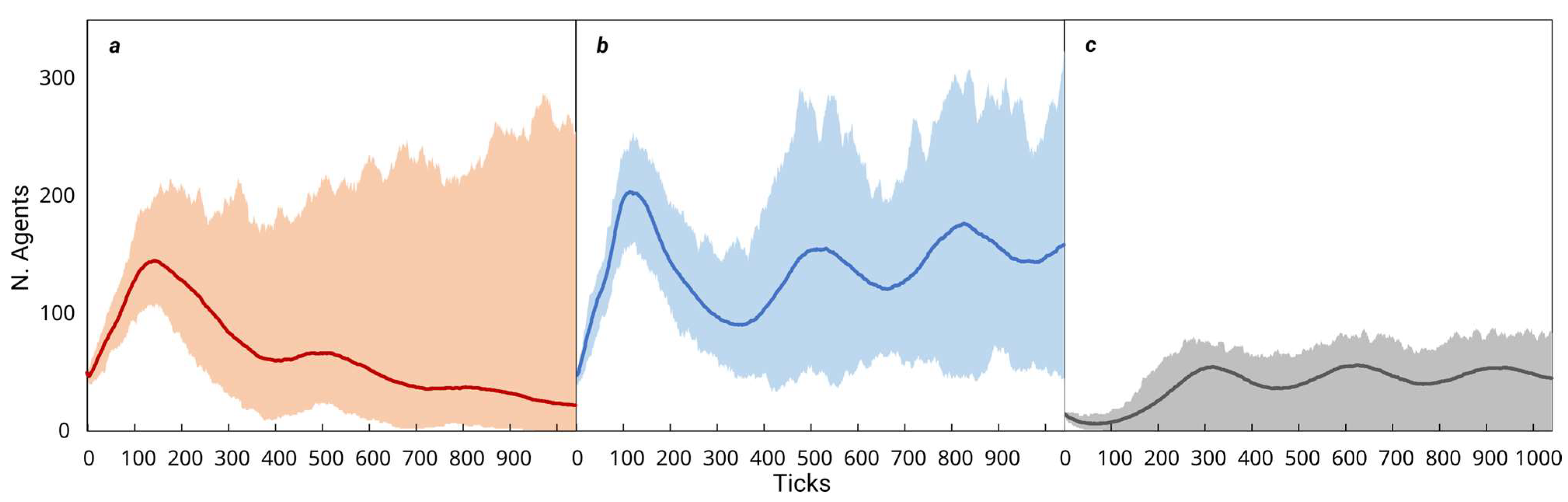
Simulations were initialized with 50 deer, 50 boar, and 15 wolves; no hunters were included. A total of 100 runs were executed under these starting conditions.

Table 2. Final abundances across runs (n = 100) in the no-hunting scenario.

Breed	Mean Final Abundance (n)	Min	Max	SD	Extinct Runs (n)
Deer	22	0	255	30	7
Boar	159	45	323	50	0
Wolves	45	0	83	16	1

reports the final abundances across runs for each breed, and Figure 1 shows the temporal ranges across runs (i.e., the minimum, mean and maximum values at each time step).

3.2. Deer-Only Hunting

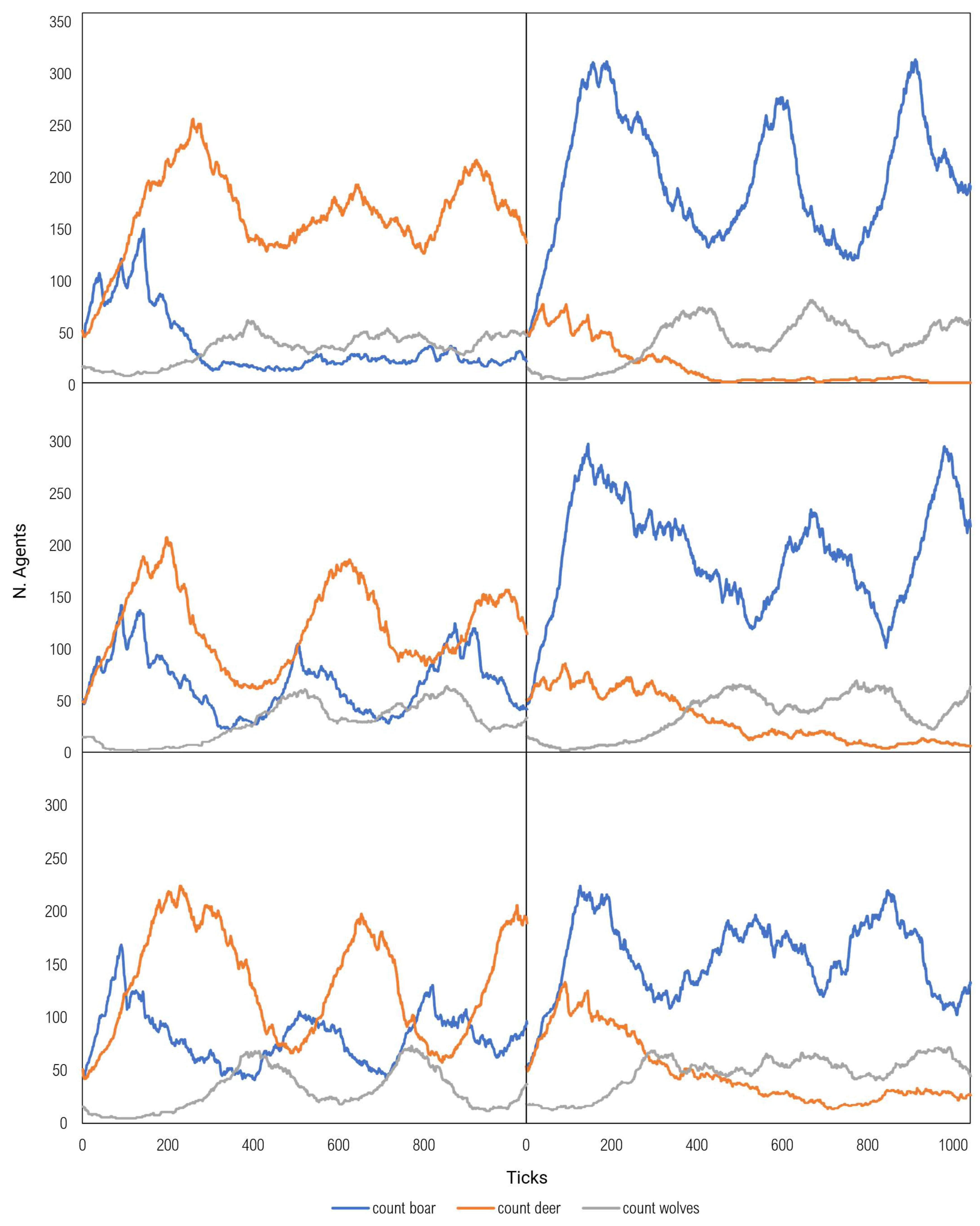
Simulations were initialized with 50 deer, 50 boar, and 15 wolves; 120 hunters were included. Deer harvest was enabled and boar harvest disabled; wolf hunting and poaching were disabled. The open season was set to 12 weeks. The deer cut-off was varied over the grid 20, 40, 60, 80, and 100, with 10 runs per level.

Table 3. Final abundances across replicates (n = 10 per scenario level) for deer-only hunting scenarios at increasing deer cut-off thresholds. Values are final abundance, mean (min–max), where min–max is the across-replicate range; extinct runs are reported as n. Final values are reported at year 20.

	Boar		Deer		Wolves
Deer Cut-off	Mean (Min–Max)	Extinct Runs (n)	Mean (Min–Max)	Extinct Runs (n)	Mean (Min–Max)	Extinct Runs (n)
20	194 (156–247)	0	1 (0–2)	7	50 (25–71)	0
40	188 (143–235)	0	6 (0–20)	2	54 (22–72)	0
60	196 (89–273)	0	10 (0–60)	2	39 (0–67)	1
80	153 (107–244)	0	5 (0–12)	3	54 (29–79)	0
100	164 (123–218)	0	16 (0–76)	2	46 (23–74)	0

reports end-of-run counts for all three species as a function of the deer cut-off. Figure 2, right, shows representative temporal trajectories for each cut-off level.

3.3. Boar-Only Hunting

Simulations were initialized with 50 deer, 50 boar, and 15 wolves; 120 hunters were included. Boar harvest was enabled and deer harvest disabled; wolf hunting and poaching were disabled. The open season was set to 12 weeks. The boar cut-off varied over the grid 20, 40, 60, 80, and 100, with 10 runs per level.

Table 4. Final abundances across replicates (n = 10 per scenario level) for boar-only hunting scenarios at increasing boar cut-off thresholds. Values are final abundance, mean (min–max), where min–max is the across-replicate range; extinct runs are reported as n. Final values are reported at year 20.

	Boar		Deer		Wolves
Boar Cut-off	Mean (Min–Max)	Extinct Runs (n)	Mean (Min–Max)	Extinct Runs (n)	Mean (Min–Max)	Extinct Runs (n)
20	11 (0–30)	3	163 (135–211)	0	44 (20–70)	0
40	31 (11–42)	0	184 (105–281)	0	38 (23–67)	0
60	42 (22–60)	0	154 (116–245)	0	52 (28–70)	0
80	56 (22–78)	0	150 (94–282)	0	49 (11–77)	0
100	74 (13–100)	0	119 (69–314)	0	42 (0–68)	1

reports end-of-run counts for all three species as a function of the boar cut-off. Figure 2, left, shows representative temporal trajectories for each cut-off level.

3.4. Hunter Density Gradient

Simulations were initialized with 50 deer, 50 boar, and 15 wolves. The number of hunters varied over 40, 60, 80, 100, 120, 140, 160, 180, 200, and 220. Deer and boar hunting were enabled; wolf hunting and poaching were disabled. The open season was set to 12 weeks. Cut-offs were fixed at deer cut-off = 150 and boar cut-off = 10. For each hunter level, 10 runs were executed.

Table 5. Final abundances across replicates (n = 10 per scenario level) at increasing initial number hunters values (40, 60, 80, 100, 120, 140, 160, 180, 200, 220). Values are the final abundance: mean (min–max), where min–max is the across-replicate range; extinct runs are reported as n.

	Boar		Deer		Wolves
n. Hunters	Mean (Min–Max)	Extinct Runs (n)	Mean (Min–Max)	Extinct Runs (n)	Mean (Min–Max)	Extinct Runs (n)
40	65 (6–152)	0	123 (55–293)	0	37 (0–53)	1
60	30 (15–57)	0	139 (102–152)	0	35 (25–43)	0
80	18 (10–35)	0	148 (139–154)	0	30 (18–43)	0
100	24 (10–53)	0	150 (147–153)	0	19 (0–27)	1
120	15 (2–62)	0	150 (148–158)	0	23 (0–30)	1
140	11 (8–17)	0	150 (147–150)	0	19 (7–33)	0
160	13 (9–25)	0	149 (148–150)	0	17 (0–27)	1
180	10 (7–13)	0	149 (147–150)	0	15 (0–21)	1
200	10 (9–12)	0	150 (148–150)	0	14 (0–22)	2
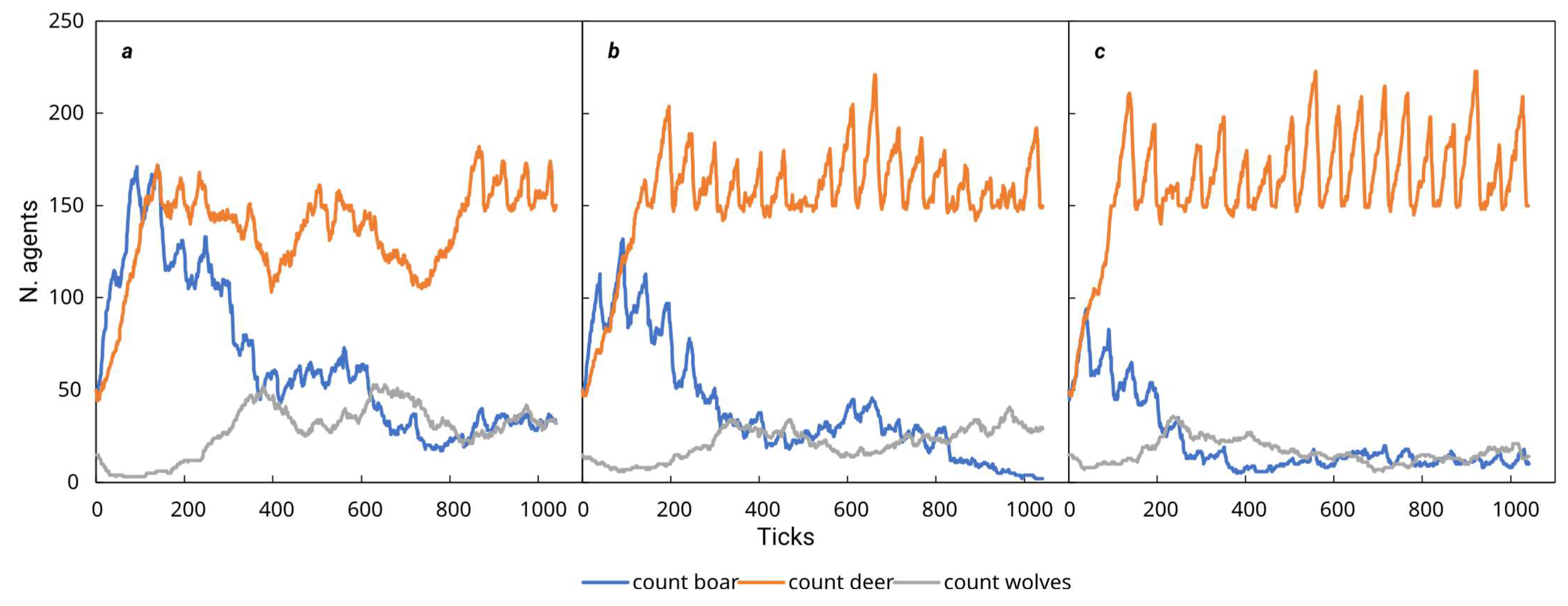
220	10 (6–11)	0	148 (143–151)	0	17 (0–34)	1

reports end-of-run counts for all three species as a function of hunter number. Figure 3 shows representative temporal trajectories for selected hunter levels.

3.5. Season Length Gradient

Simulations were initialized with 50 deer, 50 boar, 15 wolves, and 120 hunters. Deer and boar hunting were enabled; wolf hunting and poaching were disabled. The hunting season varied over 4, 8, 12, 16, and 20 weeks. Cut-offs were fixed at deer cut-off = 150 and boar cut-off = 10. For each season length, 10 runs were executed.

Table 6. Final abundances across replicates (n = 10 per scenario level) at increasing hunting season values (4, 8, 12, 16, 20 weeks); Values are the final abundance: mean (min–max); extinct runs are reported as n.

	Boar		Deer		Wolves
Hunting Season (Weeks)	Mean (Min–Max)	Extinct Runs (n)	Mean (Min–Max)	Extinct Runs (n)	Mean (Min–Max)	Extinct Runs (n)
4	42 (21–70)	0	126 (88–154)	0	41 (31–54)	0
8	17 (8–34)	0	148 (145–150)	0	31 (20–42)	0
12	17 (9–35)	0	151 (149–156)	0	18 (0–34)	1
16	15 (9–24)	0	149 (145–150)	0	16 (0–25)	1
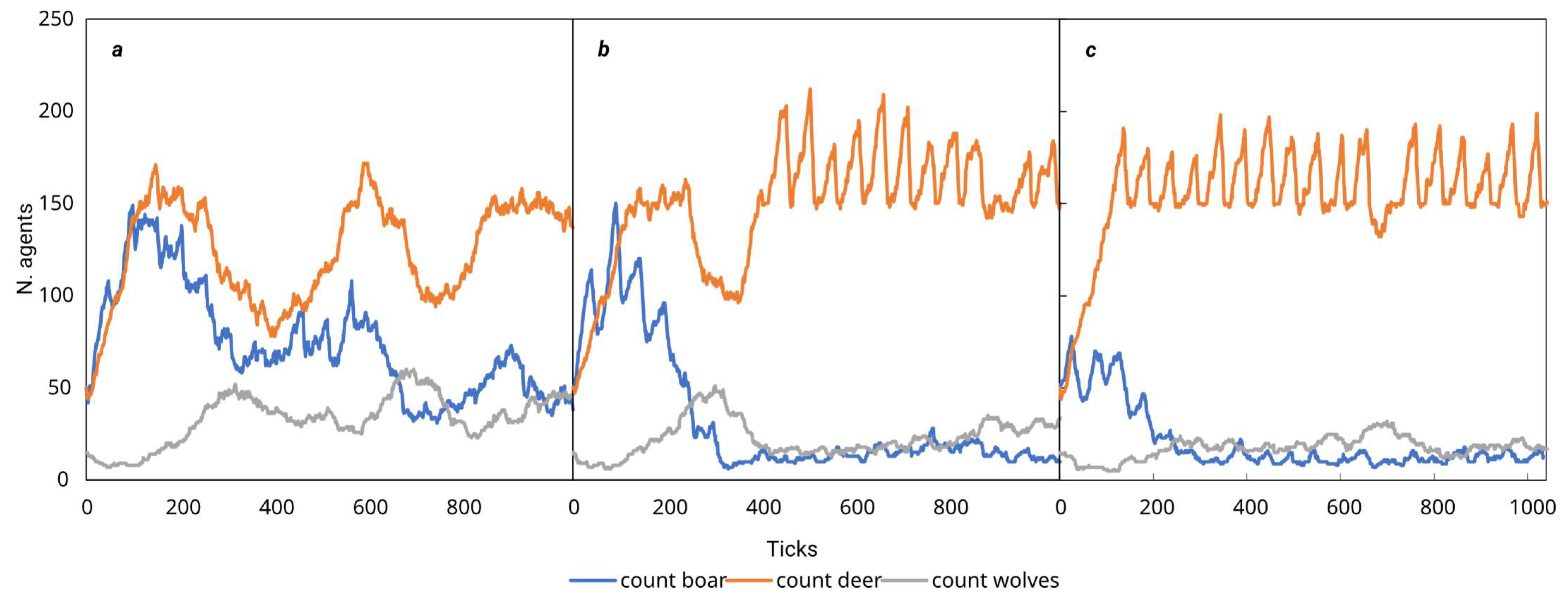
20	12 (9–17)	0	150 (146–151)	0	9 (0–19)	3

reports end-of-run counts for all three species as a function of season length. Figure 4 shows representative temporal trajectories for each level.

4. Discussion and Conclusions

Agent-based models (ABMs) are increasingly recognized not only as analytical tools in ecology but also as powerful pedagogical instruments [47]. By making assumptions explicit, representing individuals directly, and revealing system-level patterns emerging from simple behavioral rules, ABMs align well with ecology courses and wildlife-management training focused on population trajectories and human–wildlife interactions [38]. WM-Classroom v1.0 is deliberately positioned within this didactic tradition: rather than aiming for quantitative prediction or region-specific inference, it extends the classical NetLogo Wolf–Sheep model [40] into a richer, multi-species, human-influenced system that couples wolves, red deer, wild boar, and hunters on a simple 50 × 50 landscape with weekly time steps, conceived for temperate European contexts.

Consistent with this goal, the results reported are intended as illustrative dynamics conditional on the model assumptions (e.g., simplified energetics, homogeneous habitat representation, and deterministic interaction rules). We therefore use ecological terminology (e.g., oscillations, stability, resilience) in a pedagogical sense—linking explicit assumptions to emergent behavior in a controlled setting—rather than as evidence for real-world population dynamics. These simplifications also imply that some quantitative outcomes may be sensitive to how encounters and prey choice/kill success are represented.

As a teaching tool, however, the primary requirement is that trajectories remain bounded, interpretable, and reproducible across runs, so that learners can compare scenarios and trace outcomes back to explicit rules. Calibration exercises showed that the model produces qualitatively reasonable trajectories for a stylized temperate European context, providing a baseline against which teaching exercises are meaningful. Sensitivity checks and initial simulation runs confirmed stability (no crashes or pathological artifacts) and helped identify parameter ranges that yield interpretable dynamics for classroom use. The underlying model structure is then capable of underscoring a central teaching point: small parameter changes can reshape population dynamics—a hallmark of complex systems long recognized in trophic ecology [48,49]. For illustration, varying wolf-gain-from-food between 16 and 22 produced outcomes from near-certain extinction within a few ticks to unstable boom–bust cycles with very high peaks and rapid declines, with 18 serving as a reasonable reference value for the scenarios presented here. Explorations of initial population sizes maintained the predator–prey dynamics consistent with Lotka–Volterra behavior [27,28], while also making explicit a didactic assumption: herbivores experience high effective carrying capacity, since vegetation patches and initial numbers are configured to provide ready access to food without resource access limitations. This simplification supports clear classroom demonstrations of interaction rules without confounding scarcity effects.

In the absence of hunting, system behavior was governed by herbivore food availability and predator–prey interactions under the implemented rules. Boar tended to show a slight increasing trend—compatible with their higher reproduction rate—whereas deer exhibited a weaker, less defined decline with wide variation, including occasional increases in runs where wolves went extinct. Wolves were comparatively stable, settling around a mean of ~45 individuals within a narrow band. The emergent wolf/prey ratio of roughly 0.25 is higher relative to many field contexts [50], illustrating how even a small, stylized model can flag where quantitative calibration would be needed before site-level inference.

Introducing hunting on a single prey produced clear, contrasting outcomes that students can directly trace to life-history differences and rule structure. In deer-only scenarios, deer declined rapidly and often to extinction across settings—even at higher cut-offs—reflecting direct harvest mortality plus resource competition with boar, which can still grow numerically while experiencing only wolf predation. In boar-only scenarios, higher reproductive capacity made boar more persistent under the implemented rules; sustained suppression occurred only at the lowest cut-offs, whereas with less intense harvest, resource availability—and, secondarily, predation—dominated boar dynamics. In both single-prey cases, wolves remained stable but with greater fluctuations than in the no-hunting baseline, as their dynamics became more tightly coupled to one prey.

The framework is especially instructive for effort and opportunity gradients. Varying hunter density identified thresholds at which species trajectories began to shift appreciably—useful once a model is parameterized for a specific context—while also showing that beyond a certain number of active hunters, herbivores tended to cycle down toward their cut-offs during the open season and rebound outside it, with wolves declining more as hunter numbers increased via the indirect effect of prey reductions; at the highest hunter densities, wolves occasionally went extinct as a consequence of prey depletion. Manipulating hunting season length yielded analogous, predictable changes; constraints on wolves appeared more immediate and pronounced as seasons were lengthened.

For direct predator control (legal wolf removals during the open season), WM-Classroom v1.0 produced the intended predator reductions and surfaced the associated prey responses, offering a transparent demonstration of mechanism. By contrast, under poaching scenarios, the wolf population changed only modestly under the current implementation, even at relatively high weekly rates (10%). This is because the wolf-poaching rate is not applied as a per capita weekly mortality on wolves; it is encounter-conditioned and can only generate a removal when a man and a wolf are co-located on the same patch. Thus, the expected number of illegal-take events scales with the frequency of man–wolf co-location events, multiplied by wolf-poaching rate, rather than with wolf abundance alone. Under the simple random walk mixing on a 50 × 50 homogeneous grid, realized encounter frequency can be low enough that even “high” nominal rates translate into relatively few removals. Meanwhile, prey exhibited a slight long-term tendency to increase at the highest poaching settings. In a teaching context, this becomes a concrete example of how timing, thresholds, and indirect effects can generate non-obvious system responses that are useful for classroom discussion. Importantly, the magnitude of this effect is conditional on the model assumptions (e.g., the stylized demographic rates and the encounter-based representation of illegal take), and different parameterizations or alternative poaching implementations could yield stronger impacts.

Overall, the main scenario responses are broadly consistent with intuitive directional expectations: increasing harvest effort (via hunter density or season length) depresses the targeted prey and can indirectly reduce wolves through prey depletion, while legal wolf control reduces wolves by design and can release prey. Where outcomes may appear non-obvious, the reasons are traceable to explicit modeling choices (e.g., encounter-conditioned interactions). Likewise, the high baseline wolf/prey ratio flags that quantitative realism would require additional calibration and/or structural refinements before any site-level inference. For a compact overview contrasting expected directional effects of the main management levers with the corresponding qualitative outcomes observed here, see Supplementary Table S4.

More broadly, WM-Classroom v1.0 illustrates a key pedagogical strength of ABMs: by encoding simple, policy-relevant rules and running them over seasonal cycles, the model can surface interactions that are hard to communicate with equations alone but become immediate and intuitive when learners can toggle assumptions and observe outcomes. At the same time, the model provides a clear platform for discussing limitations—age/sex structure, habitat heterogeneity, and biologically grounded energetics are omitted by design—thereby preparing students to evaluate more complex models and to appreciate the demands of parameterization, calibration, validation, and uncertainty analysis.

Taken together, these features support WM-Classroom v1.0 as a didactic, modular scaffold that broadens the Wolf–Sheep paradigm into a human–wildlife context: a transparent, reproducible teaching model that makes management rules explicit in code and lets learners see how simple levers—prey cut-offs, hunter numbers, season length, and wolf control—propagate through a wolf–deer–boar system. In baseline it yields sustained predator–prey oscillations; under interventions it responds in consistent, mechanism-aligned ways. Single-prey harvest exercises highlight the deer-only vs. boar-only contrast; effort and season gradients depress prey with indirect effects on wolves; wolf control reduces predators as designed, while the poaching rates explored have little effect on wolves and only small, longer-term prey increases at the high end. Importantly, this poaching outcome is conditional on the encounter-based formulation and parameterization adopted here and is best read as a teaching example of how non-obvious responses can follow from explicit assumptions.

As a didactic tool, WM-Classroom v1.0 is intentionally simple (homogeneous habitat, abstract energetics, no age/sex structure) so that students can link assumptions to outcomes and practice scenario design, parameter sweeps, and result interpretation. This emphasis on simplicity comes with trade-offs: some quantitative patterns may be sensitive to how encounters are represented (e.g., deterministic vs. probabilistic prey choice and kill success). Because movement rules determine encounter rates and thus downstream predation and harvest dynamics, our model intentionally adopts an uncorrelated random-walk baseline for didactic transparency; future/advanced versions could test how alternative movement–ecology formulations (e.g., correlated or state-dependent diffusion, daily cycles, and attraction to key locations) modify encounter processes and management outcomes, as motivated by the movement–ecology paradigm and recent GPS-based diffusion-model classification studies [51,52]. In this context, and consistent with the intended scope of v1.0, the model is not intended to support behavioral inference (e.g., identifying movement strategies or optimal decision-making), because movement and decision rules are deliberately simplified to remain inspectable and easy to interpret in a teaching setting.

A roadmap for turning this learning resource into a tailored modeling tool capable of representing real-world ecosystems and specific contexts is possible—but nontrivial. First, strengthen the ecological structure: introduce habitat heterogeneity and seasonal resources; allow rule-based (“intelligent”) movement and dispersal across that mosaic; and make demography seasonal and age-/sex-explicit. Next, align behavior with the data by replacing deterministic diet rules with prey choice that scales with local availability and catchability, and by enriching hunter behavior (age-/sex-structured harvest, effort allocation, compliance, shot success, and adaptive switching of target species, locations, or tactics in response to recent success and local conditions). Finally, anchor the model to place: calibrate and validate against a pilot region using counts and harvest records, and run targeted sensitivity/uncertainty analyses to prioritize parameters most in need of better data. In parallel, upgrade feeding and reproduction to physical energetics and empirically grounded vital rates so the model can support quantitative inference rather than purely didactic insight.

Finally, we argue that future research may build on this stylized framework in two complementary directions.

First, the modular framework of the model allows for the integration of additional features as a foundation for interdisciplinary teaching exercises, spanning computer science (e.g., algorithmic rule design, complexity), behavioral ecology, and even social sciences, with the opportunity to theoretically explore and visualize topics including the arising conflicts between wildlife and human settlements and economic activities, the risk for poaching and illegal harvest, and other stakeholder behavior such as tourism and recreational activities actors. Second, the modular structure makes it suitable for customization toward more realistic models, should users wish to incorporate empirical data, spatial heterogeneity, age/sex structure, or calibrated energetics. In such cases, given the increasing complexity of human–wildlife systems and the rapid evolution of computational methods, future extensions could also benefit from AI-based approaches, including reinforcement learning, machine learning, and adaptive decision-making architectures [35,53]. For example, reinforcement learning may allow agents to adjust harvest effort, prey choice, or movement patterns in response to dynamic conditions rather than following hand-coded rules; similarly, recent proposals for neural-network-driven agents suggest the possibility of modeling wildlife decision-making through embedded artificial neural circuits rather than fixed behavioral routines [54]. Such techniques could support fine-grained simulations in which each agent’s behavior emerges from learned or adaptive processes, leveraging increasing computational power and algorithmic efficiency.

Exploring these directions would not only enrich the pedagogical value of the model but also open a pathway toward hybrid systems where transparent rule-based modeling and modern AI methods coexist, offering new opportunities for research, training, and decision-support. The novelty of this work lies in providing an openly reusable, classroom-oriented ABM that moves beyond single-prey Wolf–Sheep dynamics to a multi-prey European setting with human decision rules, and couples transparent management levers with reproducible scenario workflows, allowing learners to connect assumptions, rules, and outcomes in a controlled sandbox. Pursuing these steps—while archiving code, experiments, and seeds—can enable WM-Classroom v1.0 to evolve from a didactic testbed to a scenario engine that supports policy exploration and adaptive monitoring in specific European contexts.

Beyond its methodological value, WM-Classroom v1.0 already functions as a turnkey teaching and outreach tool: it can anchor high-school and undergraduate ecology labs, support training for wildlife surveyors and officers, and serve selective cull hunters in visualizing effort, cut-offs, and seasons. It also works for citizen seminars on human–wildlife interactions and decision-maker workshops, enabling transparent, low-barrier “what-if” exercises that reveal mechanism before policy.

References

1. Putman, R.; Apollonio, M.; Andersen, R. (Eds.) Ungulate Management in Europe: Problems and Practices; Cambridge University Press: Cambridge, UK, 2011. [Google Scholar]
2. Apollonio, M.; Andersen, R.; Putman, R. (Eds.) European Ungulates and Their Management in the 21st Century; Cambridge University Press: Cambridge, UK, 2010. [Google Scholar]
3. Valente, A.M.; Acevedo, P.; Figueiredo, A.M.; Fonseca, C.; Torres, R.T. Overabundant Wild Ungulate Populations in Europe: Management with Consideration of Socio-Ecological Consequences. Mamm. Rev. 2020, 50, 353–366. [Google Scholar] [CrossRef]
4. Burbaitė, L.; Csányi, S. Red Deer Population and Harvest Changes in Europe. Acta Zool. Litu. 2010, 20, 179–188. [Google Scholar] [CrossRef]
5. Massei, G.; Kindberg, J.; Licoppe, A.; Gačić, D.; Šprem, N.; Kamler, J.; Baubet, E.; Hohmann, U.; Monaco, A.; Ozoliņš, J.; et al. Wild Boar Populations up, Numbers of Hunters down? A Review of Trends and Implications for Europe. Pest Manag. Sci. 2015, 71, 492–500. [Google Scholar] [CrossRef]
6. Chapron, G.; Kaczensky, P.; Linnell, J.D.C.; Von Arx, M.; Huber, D.; Andrén, H.; López-Bao, J.V.; Adamec, M.; Álvares, F.; Anders, O.; et al. Recovery of Large Carnivores in Europe’s Modern Human-Dominated Landscapes. Science 2014, 346, 1517–1519. [Google Scholar] [CrossRef] [PubMed]
7. Ciucci, P.; Reggioni, W.; Maiorano, L.; Boitani, L. Long-Distance Dispersal of a Rescued Wolf from the Northern Apennines to the Western Alps. J. Wildl. Manag. 2009, 73, 1300–1306. [Google Scholar] [CrossRef]
8. Fabbri, E.; Caniglia, R.; Kusak, J.; Galov, A.; Gomerčić, T.; Arbanasić, H.; Huber, D.; Randi, E. Genetic Structure of Expanding Wolf (Canis lupus) Populations in Italy and Croatia, and the Early Steps of the Recolonization of the Eastern Alps. Mamm. Biol. 2014, 79, 138–148. [Google Scholar] [CrossRef]
9. Fabbri, E.; Miquel, C.; Lucchini, V.; Santini, A.; Caniglia, R.; Duchamp, C.; Weber, J.M.; Lequette, B.; Marucco, F.; Boitani, L.; et al. From the Apennines to the Alps: Colonization Genetics of the Naturally Expanding Italian Wolf (Canis lupus) Population. Mol. Ecol. 2007, 16, 1661–1671. [Google Scholar] [CrossRef]
10. Caniglia, R.; Fabbri, E.; Galaverni, M.; Milanesi, P.; Randi, E. Noninvasive Sampling and Genetic Variability, Pack Structure, and Dynamics in an Expanding Wolf Population. J. Mammal. 2014, 95, 41–59. [Google Scholar] [CrossRef]
11. Galaverni, M.; Caniglia, R.; Fabbri, E.; Milanesi, P.; Randi, E. One, No One, or One Hundred Thousand: How Many Wolves Are There Currently in Italy? Mamm. Res. 2016, 61, 13–24. [Google Scholar] [CrossRef]
12. Fležar, U.; Pičulin, A.; Bartol, M.; Stergar, M.; Sindičić, M.; Gomerčić, T.; Slijepčević, V.; Trbojević, I.; Trbojević, T.; Molinari-Jobin, A.; et al. Eurasian Lynx in the Dinaric Mountains and the Southeastern Alps, and the Need for Population Reinforcement. Cat News 2021, 14, 21–24. [Google Scholar]
13. Cunze, S.; Klimpel, S. From the Balkan towards Western Europe: Range Expansion of the Golden Jackal (Canis aureus)—A Climatic Niche Modeling Approach. Ecol. Evol. 2022, 12, e9141. [Google Scholar] [CrossRef]
14. Alexander, J.S.; Christe, P.; Zimmermann, F. Return of the Eurasian Lynx: Using Local Stakeholder Knowledge and Experiences to Inform Lynx Conservation in the French Alps. Oryx 2025, 59, 31–39. [Google Scholar] [CrossRef]
15. Recio, M.R.; Knauer, F.; Molinari-Jobin, A.; Huber, Đ.; Filacorda, S.; Jerina, K. Context-dependent Behaviour and Connectivity of Recolonizing Brown Bear Populations Identify Transboundary Conservation Challenges in Central Europe. Anim. Conserv. 2021, 24, 73–83. [Google Scholar] [CrossRef]
16. De Vivo, M. Recent Human-Bear Conflicts in Northern Italy: A Review, with Considerations of Future Perspectives. EcoEvoRxiv 2023. [Google Scholar] [CrossRef]
17. Krofel, M.; Giannatos, G.; Cirovic, D.; Stoyanov, S.; Newsome, T.M. Golden Jackal Expansion in Europe: A Case of Mesopredator Release Triggered by Continent-Wide Wolf Persecution? Hystrix Ital. J. Mammal. 2017, 28, 9–15. [Google Scholar] [CrossRef]
18. Kaczensky, P.; Ranc, N.; Hatlauf, J.; Payne, J.C.; Acosta-Pankov, L.; Álvares, F.; Andrén, H.; Andri, P.; Aragno, P.; Avanzinelli, E.; et al. Large Carnivore Distribution Maps and Population Updates 2017–2022/23; Istituto Di Ecologia Applicata (IEA): Rome, Italy, 2024. [Google Scholar]
19. Meriggi, A.; Lovari, S. A Review of Wolf Predation in Southern Europe: Does the Wolf Prefer Wild Prey to Livestock? J. Appl. Ecol. 1996, 33, 1561. [Google Scholar] [CrossRef]
20. Jędrzejewski, W.; Apollonio, M.; Jędrzejewska, B.; Kojola, I. Ungulate-Large Carnivores Relationships in Europe. In Ungulate Management in Europe—Problems and Practices; Putman, R., Apollonio, M., Andersen, R., Eds.; Cambridge University Press: Cambridge, UK, 2011; pp. 230–246. [Google Scholar]
21. Smit, C.; Putman, R. Large Herbivores as ‘Environmental Engineers’. In Ungulate Management in Europe—Problems and Practices; Putman, R., Apollonio, M., Andersen, R., Eds.; Cambridge University Press: Cambridge, UK, 2011; pp. 260–284. [Google Scholar]
22. Cromsigt, J.P.G.M.; Kuijper, D.P.J.; Adam, M.; Beschta, R.L.; Churski, M.; Eycott, A.; Kerley, G.I.H.; Mysterud, A.; Schmidt, K.; West, K. Hunting for Fear: Innovating Management of Human–Wildlife Conflicts. J. Appl. Ecol. 2013, 50, 544–549. [Google Scholar] [CrossRef]
23. Liberg, O.; Chapron, G.; Wabakken, P.; Pedersen, H.C.; Hobbs, N.T.; Sand, H. Shoot, Shovel and Shut up: Cryptic Poaching Slows Restoration of a Large Carnivore in Europe. Proc. R. Soc. B Biol. Sci. 2012, 279, 910–915. [Google Scholar] [CrossRef]
24. Milner, J.M.; Nilsen, E.B.; Andreassen, H.P. Demographic Side Effects of Selective Hunting in Ungulates and Carnivores. Conserv. Biol. 2007, 21, 36–47. [Google Scholar] [CrossRef]
25. Monaco, A.; Carnevali, L.; Toso, S. Linee Guida per La Gestione Del Cinghiale (Sus scrofa) Nelle Aree Protette. In Quaderni di Conservazione della Natura; ISPRA: Roma, Italy, 2010; Volume 34, p. 70. [Google Scholar]
26. Nowak, S.; Żmihorski, M.; Figura, M.; Stachyra, P.; Mysłajek, R.W. The Illegal Shooting and Snaring of Legally Protected Wolves in Poland. Biol. Conserv. 2021, 264, 109367. [Google Scholar] [CrossRef]
27. Lotka, A.J. Elements of Physical Biology; Williams & Wilkins: Baltimore, MD, USA, 1925. [Google Scholar]
28. Volterra, V. Variazioni e Fluttuazioni Del Numero d’individui in Specie Animali Conviventi; Memorie Della Classe di Scienze Fisiche, Matematiche e Naturali; Societá Anonima Tipografica “Leonardo da Vinci”; Reale Accademia Nazionale dei Lincei: Rome, Italy, 1927. [Google Scholar]
29. Caswell, H. Matrix Population Models. In Encyclopedia of Environmetrics; Wiley: Hoboken, NJ, USA, 2006. [Google Scholar]
30. Millspaugh, J.; Thompson, F. Models for Planning Wildlife Conservation in Large Landscapes; Elsevier: Amsterdam, The Netherlands, 2009. [Google Scholar]
31. Schaub, M.; Abadi, F. Integrated Population Models: A Novel Analysis Framework for Deeper Insights into Population Dynamics. J. Ornithol. 2011, 152, 227–237. [Google Scholar] [CrossRef]
32. Railsback, S.F.; Grimm, V. Agent-Based and Individual-Based Modeling: A Practical Introduction; Princeton University Press: Princeton, NJ, USA, 2019. [Google Scholar]
33. Musters, C.J.M.; DeAngelis, D.L.; Harvey, J.A.; Mooij, W.M.; van Bodegom, P.M.; de Snoo, G.R. Enhancing the Predictability of Ecology in a Changing World: A Call for an Organism-Based Approach. Front. Appl. Math Stat. 2023, 9, 1046185. [Google Scholar] [CrossRef]
34. Zhang, B.; DeAngelis, D.L. An Overview of Agent-Based Models in Plant Biology and Ecology. Ann. Bot. 2020, 126, 539–557. [Google Scholar] [CrossRef] [PubMed]
35. DeAngelis, D.L.; Mooij, W.M. Individual-Based Modeling of Ecological and Evolutionary Processes. Annu. Rev. Ecol. Evol. Syst. 2005, 36, 147–168. [Google Scholar] [CrossRef]
36. Crooks, A.; Malleson, N.; Manley, E.; Heppenstall, A.J. Agent-Based Modelling & Geographical Information Systems: A Practical Primer, 1st ed.; Rojek, R., Nightingale, J., Haw, K., Leigh, R., Eds.; SAGE Publications: London, UK, 2019. [Google Scholar]
37. Bousquet, F.; Le Page, C. Multi-Agent Simulations and Ecosystem Management: A Review. Ecol. Modell. 2004, 176, 313–332. [Google Scholar] [CrossRef]
38. McLane, A.J.; Semeniuk, C.; McDermid, G.J.; Marceau, D.J. The Role of Agent-Based Models in Wildlife Ecology and Management. Ecol. Modell. 2011, 222, 1544–1556. [Google Scholar] [CrossRef]
39. Tisue, S.; Wilensky, U. NetLogo: Design and Implementation of a Multi-Agent Modeling Environment. In Proceedings of the Agent 2004 Conference on Social Dynamics: Interaction, Reflexivity and Emergence, Chicago, IL, USA, 7–9 October 2004; p. 20. [Google Scholar]
40. Wilensky, U. NetLogo Wolf Sheep Predation Model. 1997. Available online: http://ccl.northwestern.edu/netlogo/models/WolfSheepPredation (accessed on 12 December 2025).
41. Coste, C. Hunting-and-Poaching (NetLogo Model, ID 7525). 2024. Available online: https://modelingcommons.org/browse/one_model/7525 (accessed on 2 December 2025).
42. Grimm, V.; Berger, U.; DeAngelis, D.L.; Polhill, J.G.; Giske, J.; Railsback, S.F. The ODD Protocol: A Review and First Update. Ecol. Modell. 2010, 221, 2760–2768. [Google Scholar] [CrossRef]
43. Grimm, V.; Railsback, S.F.; Vincenot, C.E.; Berger, U.; Gallagher, C.; DeAngelis, D.L.; Edmonds, B.; Ge, J.; Giske, J.; Groeneveld, J.; et al. The ODD Protocol for Describing Agent-Based and Other Simulation Models: A Second Update to Improve Clarity, Replication, and Structural Realism. J. Artif. Soc. Soc. Simul. 2020, 23, 7. [Google Scholar] [CrossRef]
44. Apollonio, M.; Mattioli, L.; Scandura, M. Wolves in the Casentinesi Forests: Insights for Wolf Conservation in Italy from a Protected Area with a Rich Wild Prey Community. Biol. Conserv. 2004, 120, 249–260. [Google Scholar] [CrossRef]
45. Bassi, E.; Willis, S.G.; Passilongo, D.; Mattioli, L.; Apollonio, M. Predicting the Spatial Distribution of Wolf (Canis lupus) Breeding Areas in a Mountainous Region of Central Italy. PLoS ONE 2015, 10, e0124698. [Google Scholar] [CrossRef]
46. Mattioli, L.; Capitani, C.; Gazzola, A.; Scandura, M.; Apollonio, M. Prey Selection and Dietary Response by Wolves in a High-Density Multi-Species Ungulate Community. Eur. J. Wildl. Res. 2011, 57, 909–922. [Google Scholar] [CrossRef]
47. Hsiao, L.; Lee, I.; Klopfer, E. Making Sense of Models: How Teachers Use Agent-based Modeling to Advance Mechanistic Reasoning. Br. J. Educ. Technol. 2019, 50, 2203–2216. [Google Scholar] [CrossRef]
48. Elton, C.S. Animal Ecology; Macmillan Co: New York, NY, USA, 1927. [Google Scholar]
49. Odum, E.P.; Barrett, G.W. Fundamentals of Ecology, 5th ed.; Brooks/Cole: San Francisco, CA, USA, 2004. [Google Scholar]
50. Eberhardt, L.L.; Peterson, R.O. Predicting the Wolf-Prey Equilibrium Point. Can. J. Zool. 1999, 77, 494–498. [Google Scholar] [CrossRef]
51. Nathan, R.; Getz, W.M.; Revilla, E.; Holyoak, M.; Kadmon, R.; Saltz, D.; Smouse, P.E. A Movement Ecology Paradigm for Unifying Organismal Movement Research. Proc. Natl. Acad. Sci. USA 2008, 105, 19052. [Google Scholar] [CrossRef]
52. Meyer, P.G.; Cherstvy, A.G.; Seckler, H.; Hering, R.; Blaum, N.; Jeltsch, F.; Metzler, R. Directedeness, Correlations, and Daily Cycles in Springbok Motion: From Data via Stochastic Models to Movement Prediction. Phys. Rev. Res. 2023, 5, 043129. [Google Scholar] [CrossRef]
53. Strannegård, C.; Xu, W.; Engsner, N.; Endler, J.A. Combining Evolution and Learning in Computational Ecosystems. J. Artif. Gen. Intell. 2020, 11, 1–37. [Google Scholar] [CrossRef]
54. Strannegård, C.; Palak, M.; Engsner, N.; Stocco, A.; Antonelli, A.; Silvestro, D. Predicting Ecosystem Resilience Using Multi-Agent Reinforcement Learning. bioRxiv 2025. bioRxiv:2025.06.07.658424. [Google Scholar] [CrossRef]
55. Brogi, R.; Merli, E.; Grignolio, S.; Chirichella, R.; Bottero, E.; Apollonio, M. It is time to mate: Population-level plasticity of wild boar reproductive timing and synchrony in a changing environment. Curr. Zool. 2022, 68, 371–380. [Google Scholar] [CrossRef]
56. Capitani, C.; Bertelli, I.; Varuzza, P. A comparative analysis of wolf (Canis lupus) diet in three different Italian ecosystems. Mamm Biol 2004, 69, 1–10. [Google Scholar] [CrossRef]
57. Iacolina, L.; Scandura, M.; Bongi, P.; Apollonio, M. Nonkin associations in wild boar social units. J. Mammal. 2009, 90, 666–674. [Google Scholar] [CrossRef]
58. Meriggi, A.; Brangi, A.; Matteucci, C.; Sacchi, O. The feeding habits of wolves in relation to large prey availability in northern italy. Ecography 1996, 19, 287–295. [Google Scholar] [CrossRef]
59. Zanni, M.; Brivio, F.; Grignolio, S.; Apollonio, M. Estimation of spatial and temporal overlap in three ungulate species in a mediterranean environment. Mamm. Res. 2021, 66, 149–162. [Google Scholar] [CrossRef]
60. Clutton-Brock, T.H.; Guinness, F.E.; Albon, S.D.; Barrett, P. Red Deer: Behavior and Ecology of Two Sexes; University of Chicago Press: Chicago, IL, USA, 1982. [Google Scholar]
61. Keuling, O.; Baubet, E.; Duscher, A.; Ebert, C.; Fischer, C.; Monaco, A.; Podgórski, T.; Prévot, C.; Ronnenberg, K.; Sodeikat, G.; et al. Mortality rates of wild boar Sus scrofa L. In central Europe. Eur. J. Wildl. Res. 2013, 59, 805–814. [Google Scholar] [CrossRef]
62. Massei, G.; Genov, P. The Environmental Impact of Wild Boar. Galemys: Boletín informativo de la Sociedad Española para la conservación y estudio de los mamíferos. Galemys 2004, 16, 135–145. [Google Scholar] [CrossRef]
63. Mech, L.D.; Boitani, L. (Eds.) Wolves: Behavior, Ecology, and Conservation; University of Chicago Press: Chicago, IL, USA, 2010. [Google Scholar]
Figure 1. Range of variation over time in the number of agents for the three breeds in 100 simulations with identical initial parameters and no hunting ((a): deer; (b): boar; (c): wolf).
Wild 03 00008 g001
Figure 2. Time series of deer, boar, and wolves under prey-specific hunting, with hunting season = 12 weeks. Left column, top to bottom: Boar-only harvest with boar cut-off set to 100, 60, 20 (one representative run per level). Right column, top to bottom: Deer-only harvest with deer cut-off set to 100, 60, 20 (one representative run per level).
Wild 03 00008 g002
Figure 3. Time series of deer, boar, and wolves under deer + boar hunting with hunting season = 12 weeks, deer cut-off = 150, boar cut-off = 10, and initial number hunters set to 80 (a), 120 (b), and 160 (c).
Wild 03 00008 g003
Figure 4. Time series of deer, boar, and wolves under deer + boar hunting with initial-number-hunters = 120, deer-cut-off = 150, boar-cut-off = 10, and hunting-season set to (a) 4, (b) 12, and (c) 20 weeks.
Wild 03 00008 g004