Energy Management Strategy for a Bioethanol Isolated Hybrid System: Simulations and Experiments

Abstract

Renewable energy sources have significant advantages both from the environmental and the economic point of view. Additionally, renewable energy sources can contribute significantly to the development of isolated areas that currently have no connection to the electricity supply network. In order to make efficient use of these energy sources, it is necessary to develop appropriate energy management strategies. This work presents an energy management strategy for an isolated hybrid renewable energy system with hydrogen production from bioethanol reforming. The system is based on wind-solar energy, batteries and a bioethanol reformer, which produces hydrogen to feed a fuel cell system. Bioethanol can contribute to the development of isolated areas with surplus agricultural production, which can be used to produce bioethanol. The energy management strategy takes the form of a state machine and tries to maximize autonomy time while minimizing recharging time. The proposed rule-based strategy has been validated both by simulation and experimentally in a scale laboratory station. Both tests have shown the viability of the proposed strategy complying with the specifications imposed and a good agreement between experimental and simulation results.

1. Introduction

Nowadays, energy production from renewable sources, like solar or wind energy and biofuels, is receiving worldwide attention. Fossil fuels have low efficiency with a high level of emissions that contribute to global warming. In addition, the exploitation of hydrocarbons involves serious social and environmental consequences. Renewable energy sources (RESs) are technologies that are contributing significantly to the diversification of the energy matrix due to their sustainability characteristics and low emissions. However, a common drawback is the unpredictable nature and climate dependence of the RESs, which is more serious in isolated systems that do not have a connection to the electricity grid. However, this problem can be overcome by combining different energy sources and using energy storage units. Such systems are called hybrid renewable energy systems (HRESs) [1,2].

The combination of photovoltaic (PV) and wind energy generation has been reported in several works for isolated applications [3,4]. However, hybrid systems need energy storage elements to ensure the power balance in the face of sudden changes in power demand/generation. For short-term energy storage, batteries are the most common storage devices due to the high round-trip efficiency and relatively fast time response, which allow mitigating the harmful effect of RESs fluctuations [5]. However, during long periods with low generation, an isolated HRES requires a complementary energy source to guarantee the reliability of the system. In our system, this role is fulfilled by polymer electrolyte membrane fuel cells (PEMFCs). PEMFCs generate electricity using hydrogen as the raw material with a higher efficiency than other technologies (e.g., internal combustion engines). Hybridization between fuel cells and wind-solar sources has been reported in several works [6,7].

Regarding the production of hydrogen needed to operate the PEMFC, electrolysis is a widely-used method [8]. However, an interesting alternative is bioethanol reforming. The advantages of bioethanol, compared with other fuels, are high hydrogen content, availability, low toxicity and safe storage and handling. Bioethanol reforming for hydrogen production to feed a PEMFC is reported in several works [9,10,11]. In addition, bioethanol can be produced by fermentation of biomass sources such as agricultural residues, forestry, livestock and urban organic material [12,13]. Furthermore, bioethanol production in agricultural countries like Argentina is significant and is continuously growing as a result of environmental policies that encourage the change of the energy matrix, making it less dependent on fossil fuels [14]. Therefore, bioethanol reforming is a promising alternative to produce the hydrogen required by the PEMFC. Henceforth, the reformer that produces hydrogen from bioethanol, with additional cleaning stages, will be called the bioethanol reformer subsystem (BRS).

The energy management strategy (EMS) is the algorithm in charge of the operation of the HRES subsystems. The EMS establishes in real time the power references of each subsystem to comply with the load balance and optimize the performance of HRES. Different approaches of EMS in hybrid systems with multiple renewable energy sources are found in the literature. A complete review can be found in [15]. Rule-based strategies are widely used due to the simplicity of their implementation and their low computational cost. The EMS can be represented by a set of possible states in which the power references for each element are defined. The system switches between the states according to heuristic rules [16]. More complex strategies based on model predictive control (MPC) and optimization strategies have been widely used in power management applications in recent years [17,18]. However, this kind of methodology generally involves high implementation difficulties. Three EMSs based on switching between different modes are presented and compared in [19]. The authors applied the proposed EMS to an isolated power system based on a PV array and wind generators that use water electrolysis to produce hydrogen for future use in a PEMFC. In [20], a rule-based EMS implemented through a state machine approach was proposed for a wind/PV/BRS/Fuel Cell system. This strategy is compared in [21] with another that uses the concept of a receding horizon with predictions of the future generation from the renewable sources, the future load and the state of charge in the battery bank. In [17], the authors studied the role of EMSs in microgrids with water electrolysis and presented experimental results. In [22], the authors proposed an energy management strategy based on multiple operating states for a DC microgrid, which is comprised of a PV array, a PEMFC system and a battery bank. This strategy can share the power properly and keep the bus voltage at the desired value under different operating states. However, the design of EMSs for isolated HRESs with bioethanol-based hydrogen production from theoretical and experimental approaches is not addressed in the literature.

This work presents an EMS for an isolated HRES composed of wind-PV generation, a battery bank and a PEMFC, where the hydrogen required by the PEMFC is produced from bioethanol reforming. The proposed EMS is based on a finite state machine. First, the EMS is evaluated by simulation using historical data over long periods of time to study the reliability of the strategy during different scenarios. Then, an experimental validation of the EMS is carried out using the profiles of a typical day. For this purpose, a methodology is proposed to scale the initial scenario so that the tests can be performed in the laboratory. This methodology preserves the most relevant energy-flow characteristics. Finally, the experimental results obtained are compared with those corresponding to the simulations.

The organization of the rest of this paper can be summarized as follows. In Section 2, a description of the HRES and the corresponding mathematical models are addressed. Section 3 describes the proposed energy management strategy. In Section 4.1, a possible real scenario is described. In Section 4.2, the simulations results of the proposed EMS are shown. In Section 4.3, the laboratory test station is described, and in Section 4.4, the scaling methodology is presented. The experimental results are shown and discussed in Section 4.5. Finally, the conclusions and future work lines for further research are stated in Section 5.

2. System Description

The topology of the HRES under study in this work is shown in Figure 1. The wind and PV sources, as well as the PEMFC are connected to the DC bus via unidirectional DC-DC boost converters. In the case of the battery, a bidirectional boost DC-DC converter must be used to ensure the charging and discharging mode. The power references are imposed by the EMS (explained in detail in Section 3). The size of the system was determined using the sizing methodology presented in [23], where the developed methodology allows one to obtain a sizing for different scenarios and to fulfil the performance specifications. The characteristics of the components of the system in terms of their rated powers or capacities are summarized in

Table 1. HRES case study description.

HRES Component	Rated Power/Capacity
Wind subsystem	$4.5$ kW
Solar subsystem	$6{\mathrm{kW}}_{\mathrm{p}}$
Energy storage subsystem	$8.11\mathrm{kWh}$
PEM fuel cell subsystem	$4.8$ kW
Bioethanol reformer subsystem (heater)	$1.55$ kW
Load power demand	$4.1{\mathrm{kW}}_{\mathrm{p}}$

. The power converters in the model are assumed ideal and perfectly controlled.

2.1. Bioethanol Reformer Subsystem

Steam reforming is one of the most widely-used methods to obtain hydrogen from bioethanol because it achieves a high concentration of hydrogen, necessary to feed the PEM fuel cell subsystem [24]. The main reactor is the ethanol steam reformer (ESR), where most of the conversion of bioethanol into hydrogen takes place. Then, a clean stage composed of three water-gas shift reactors (WGS) removes the carbon monoxide that can damage the catalyst of the fuel cell [25]. The endothermic condition of the ESR reaction implies the supply of heat. A solution reported in [26] consists of burning a portion of the bioethanol in a separate reactor to provide the reaction heat from the gases obtained. However, this solution has a negative impact on the efficiency due to the extra bioethanol consumption. To avoid this situation, the burner is replaced by an electric heating subsystem, which is powered from the DC bus [27].

The amount of heat needed in the reaction is $\Delta H_{298}^0=254.8{\mathrm{kJ}\mathrm{mol}}^{-1}$ [23]. The power required by the heater ($P_h$) can be obtained from the stoichiometric equation of the reaction:

$$P_h=\frac{W_{H_2}\Delta H_{298}^0}{4},$$

(1)

where $W_{H_2}$ is the rate of hydrogen consumed by the PEMFC.

2.2. PEM Fuel Cell Subsystem

In this work, the voltage-current and power-current curves in the data sheet of a $1.2\mathrm{kW}$ Nexa module are used to build the model [28]. The rate of hydrogen consumed in the electrochemical reaction in the PEMFC anode can be approximated by the following expression depending on the current ($I_{fc}$):

$$W_{H_2}=\frac{{\eta }_{F,fc}n}{2F}{I}_{fc},$$

(2)

where $W_{H_2}$ is the rate of hydrogen reacted, ${\eta }_{F,fc}$ is the Faraday efficiency (90–95%), n is the number of cells in the FC (a typical value of 26 cells is considered) and $F=96485\mathrm{C}{\mathrm{mol}}^{-1}$ is the Faraday number. This hydrogen flow is supplied by the BRS presented in Section 2.1.

The power of the FC must be maintained within certain limits. The upper limit is the nominal power of FC, while the minimum is fixed to guarantee a minimum efficiency. Therefore, the following constraints can be formulated:

$$P_{fc}^{min}\le P_{fc}\le P_{fc}^{max},$$

(3)

with a $P_{fc}^{min}=300\mathrm{W}$ and a $P_{fc}^{max}=1200\mathrm{W}$. In addition, the PEMFC power cannot be increased faster than a certain rise rate power ($\Delta P_{fc}^{max}$) to avoid a lack of reactants and the power cannot be decreased faster than a certain fall rate power ($\Delta P_{fc}^{min}$) to prevent overpressure in the PEMFC [29]. Therefore, the following constraints are added:

$$\Delta P_{fc}^{min}\le \Delta P_{fc}\le \Delta P_{fc}^{max},$$

(4)

where $\Delta P_{fc}=P_{fc}\left(t\right)-P_{fc}(t-\Delta T)$ and $\Delta T$ is the sample time. The values used are $\Delta P_{fc}^{max}=0.1P_{fc}^{max}$ and $\Delta P_{fc}^{min}=-0.1P_{fc}^{max}$ [30].

2.3. Wind Power Subsystem

The maximum power that a wind turbine is able to generate can be expressed by:

$$P_w=\frac{1}{2}{C}_p(\lambda ,\beta ){\rho }_a\pi r^2{v}^3,$$

(5)

where r is the radius of the blades, ${\rho }_a$ is the air density and v is the wind velocity. The power coefficient ($C_p$) expresses the efficiency of the turbine with respect to the wind power available. The coefficient $C_P$ is a function of $\lambda$ and the blade pitch angle $\beta$, where $\lambda =r{\omega }_m/v$ and ${\omega }_m$ is the speed angle of the turbine shaft. Then, $C_p$ can be expressed by [31]:

$$C_p(\lambda ,\beta )=\frac{1}{2}\left(\frac{r{C}_f}{\lambda }-0.022\beta -2\right)e^{-0.255\frac{r{C}_f}{\lambda }},$$

(6)

where $C_f$ is a design constant of the blades.

When the wind speed is below the cut-in speed ($v_{w,cin}$), no power is generated. Above this value, the generated power responds to Equation (5). When the rated power of the machine ($P_{w,r}$) is reached at $v_{w,r}$, the output power must be operated at constant output power in order to prevent damage. The turbine must be stopped if the wind speed is higher than its cut-out limit ($v_{w,cout}$) [32]. In this work, a perfect control of the power delivered by the turbine is assumed, working in maximum power point tracking (MPPT) or load power tracking (LPT). The values of the parameters used in the model are presented in

Table 2. Parameters of each wind turbine ($4.5{\mathrm{kW}}_{\mathrm{p}}$).

Parameter	Value
${\rho }_a$	1.2 ${\mathrm{kg}/\mathrm{m}}^3$
r	1.6 m
$C_{p,max}$	0.59
$v_{w,r}$	12 $\mathrm{m}/\mathrm{s}$
$v_{w,cin}$	3 $\mathrm{m}/\mathrm{s}$
$v_{w,cout}$	20 $\mathrm{m}/\mathrm{s}$

. The value for the power coefficient is $C_p(\lambda ,\beta )=0.59$, resulting in a $4.5{\mathrm{kW}}_{\mathrm{p}}$ wind turbine.

2.4. Solar Power Subsystem

The solar power subsystem is composed of a PV array connected to the DC bus through a DC/DC power converter. A PV array is a group of several PV panels, which are electrically connected in series and parallel circuits to generate the required voltage and power. In turn, each PV panel is composed of several PV cells.

PV cells have voltage-current and power-current nonlinear characteristics, strongly dependent on radiation and temperature. A possible expression for the output current $I_{pv}$ of a PV cell is given by [33]:

$$I_{pv}=I_{ph}-I_{rs}\left(exp\left(\frac{q\left(V_{pv}+I_{pv}{R}_s\right)}{A_{c}KT}\right)-1\right),$$

(7)

where $I_{ph}$ is the generated current under a reference radiation, $I_{rs}$ is the cell reverse saturation current, $V_{pv}$ is the voltage level on the PV cell terminals, q is the charge of an electron, $R_s$ is the intrinsic cell resistance, $A_c$ is the cell deviation from the ideal p-n junction characteristic, K is the Boltzmann constant and T is the cell temperature. The photocurrent depends on radiation and temperature according to the following expression:

$$I_{ph}=(I_{sc}+K_l(T-T_r))\nu /1000,$$

(8)

where $I_{sc}$ is the short-circuit cell current at the reference temperature and radiation, $K_l$ is the short-circuit current temperature coefficient and $\nu$ is the measured radiation expressed in ${\mathrm{W}\mathrm{m}}^{-2}$.

The reverse saturation current depends on temperature according to the following expression:

$$I_{rs}=I_{or}{\left(\frac{T}{T_{ref}}\right)}^{3}exp\left(\frac{q{E}_{go}(1/T_r-1/T)}{K{A}_c}\right),$$

(9)

where $I_{or}$ is the reverse saturation current at the reference temperature $T_{ref}$ and $E_{go}$ is the band-gap energy of the semiconductor used in the cell. Thus, the available current for a PV panel can be expressed as follows:

$$I_{PV}=n_p{I}_{ph}-n_p{I}_{rs}\left(exp\left(\frac{q\left(V_{PV}+I_{pv}{R}_s\right)}{n_s{A}_{c}KT}\right)-1\right),$$

(10)

where $V_{PV}$ is the voltage level in the PV panel terminals, $n_p$ is the number of parallel strings and $n_s$ is the number of serial connected cells per string. Therefore, the available power generation from a PV panel is:

$$P_{pv}=V_{PV}{I}_{PV}.$$

(11)

The values of the constants used in the model are given in

Table 3. Parameters of each PV panel ($250{\mathrm{W}}_{\mathrm{p}}$).

Parameter	Value
q	$1.6\times {10}^{-19}C$
$A_c$	$1.6$
K	$1.3805\times {10}^{-23}\mathrm{Nm}{\mathrm{K}}^{-1}$
$K_l$	$0.0017A{}^{\circ }$C${}^{-1}$
$I_{or}$	$2.0793\times {10}^{-6}\mathrm{A}$
$T_{ref}$	$301.18\mathrm{K}$
$E_{go}$	$1.10\mathrm{V}$
$I_{sc}$	$3.27\mathrm{A}$
$n_p$	1
$n_s$	60
number of PV panels per module	4

and correspond to a commercial panel of 250 ${\mathrm{W}}_{\mathrm{p}}$. In this work, four PV panels are connected in parallel in a single PV module, obtaining a peak power for each module of $1{\mathrm{kW}}_{\mathrm{p}}$. Then, the sizing strategy calculates how many modules to install in the system. The maximum PV available power $P_{pv}$ at each instant is obtained through an MPPT algorithm.

2.5. Energy Storage Subsystem

The natural variability of wind-solar power jointly with the isolated application implies the need to include energy storage devices having a reliable power supply. Batteries are the most widely-used energy storage devices in isolated applications due to their high specific energy.

In this work, the energy storage subsystem (ESS) is composed of batteries. The model presented in [34], integrated in the SimPowerSystems toolbox of MATLAB, is used. This model is based on an equivalent circuit with a variable voltage source and a serial internal resistance. The variable voltage source and the internal resistance depend on the battery state of charge ($SoC$), which represents the remaining capacity still available to be discharged from the battery [35]. The $SoC$ can be defined as follows:

$$SoC\left(t\right)=So{C}_{ini}-\frac{1}{C_{bat}}{\int }_{t_0}^t{i}_{bat}dt,$$

(12)

where $C_{bat}$ is the capacity of the bank of batteries. The $SoC$ must be kept within certain limits to ensure good performance and maximize battery lifetime. The main characteristics of the batteries used are in

Table 4. Parameters of each unit of the energy storage subsystem ($1352\mathrm{Wh}$).

Parameter	Value
Capacity of each battery $C_{bat}$	$104\mathrm{Ah}/1352\mathrm{Wh}$
Rated voltage $V_{bat}^r$	$13\mathrm{V}$

.

3. Energy Management Strategy

The energy management strategy is the algorithm that controls the power references of the local controllers to guarantee the power balance in the DC bus while complying with the constraints of the system. The power balance in the DC bus can be expressed as follows:

$$P_w\left(t\right)+P_{pv}\left(t\right)+P_{fc}\left(t\right)+P_{bat}\left(t\right)-P_h\left(t\right)-P_{load}\left(t\right)=0,$$

(13)

where $P_w$, $P_{pv}$, $P_{fc}$ and $P_{bat}$ are the power provided by the wind turbines, the PV array, the fuel cell and the batteries, respectively, while $P_h$ and $P_{load}$ are the power consumed by the electric heater and the load, respectively. The power delivered by the batteries is considered positive in the discharge mode and negative when charging.

Two important specifications are introduced for the design of the EMS. The first, and the most important in this type of isolated systems, is the autonomy time. It refers to the capacity of the batteries to support the full load demand until it falls below the minimum $SoC$ level. When the load demand exceeds the generation provided by the RESs and the fuel cell, the batteries allow meeting the power balance until the $SoC$ falls below $So{C}_{min}$. When this situation occurs, only the vital loads ($P_{load}^{vital}$) are fed. The vital loads are the essential loads that assure the minimum performance of the system. The second specification introduced is the recharge time, which is defined as the time the batteries require to recover the capacity to supply all the regular power demand.

According to these specifications, some basic principles are defined to design the EMS:

• The RESs deliver their maximum power (MPPT mode), while the batteries do not exceed the maximum charge level.
• When the battery reaches its maximum $SoC$ level, the RESs change to LPT mode, where the power reference follows the load demand.
• Minimize the battery cycles of charging and discharging to preserve their lifetime.
• The fuel cell provides energy to the DC bus during low RES generation periods and maintains the $SoC$ of the batteries at a desirable level.

The EMS is implemented using a finite state machine approach. This tool is widely used in decision making algorithms and EMSs [36]. A state machine makes a transition between modes (states) according to specific events. In each state, the power references for the local controllers are defined. The algorithm implemented can be represented by a statechart, which is a graphical way to describe a finite state machine, as shown in Figure 2.

The description of the events is given in

Table 5. Description of the events in the set $\Sigma$.

Event	Description
1	$SoC\ge So{C}_{L1}$
2	$SoC\le (So{C}_{L1}-So{C}_{th})$
3	$SoC\le So{C}_{min}$
4	$SoC\ge So{C}_{max}$
5	$p_{load}^{req}\le p_{ren}^{av}$

, while the mathematical description of each state is presented below:

• State 1:

  $$\begin{array}{ccc}\hfill P_{load}^{del}& =& P_{load}^{req},\hfill \end{array}$$

  (14)

  $$\begin{array}{ccc}\hfill P_{res}^{ref}& =& P_{res}^{av},\hfill \end{array}$$

  (15)

  $$\begin{array}{ccc}\hfill P_{fc}^{ref}& =& 0,\hfill \end{array}$$

  (16)

  $$\begin{array}{ccc}\hfill P_{bat}^{ref}& =& P_{load}^{del}-P_{res}^{ref},\hfill \end{array}$$

  (17)
• State 2:

  $$\begin{array}{ccc}\hfill P_{load}^{del}& =& P_{load}^{req},\hfill \end{array}$$

  (18)

  $$\begin{array}{ccc}\hfill P_{res}^{ref}& =& P_{res}^{av},\hfill \end{array}$$

  (19)

  $$\begin{array}{ccc}\hfill P_{fc}^{ref}& =& P_{load}^{del}+P_{bat}^{ch}+P_h-P_{res}^{ref},\hfill \end{array}$$

  (20)

  $$\begin{array}{ccc}\hfill P_{bat}^{ref}& =& P_{load}^{del}+P_h-P_{res}^{ref}-P_{fc}^{ref},\hfill \end{array}$$

  (21)
• State 3:

  $$\begin{array}{ccc}\hfill P_{load}^{del}& =& P_{load}^{req},\hfill \end{array}$$

  (22)

  $$\begin{array}{ccc}\hfill P_{res}^{ref}& =& P_{res}^{av},\hfill \end{array}$$

  (23)

  $$\begin{array}{ccc}\hfill P_{fc}^{ref}& =& P_{load}^{del}+P_h-P_{res}^{ref},\hfill \end{array}$$

  (24)

  $$\begin{array}{ccc}\hfill P_{bat}^{ref}& =& P_{load}^{del}+P_h-P_{res}^{ref}-P_{fc}^{ref},\hfill \end{array}$$

  (25)
• State 4:

  $$\begin{array}{ccc}\hfill P_{load}^{del}& =& P_{load}^{req},\hfill \end{array}$$

  (26)

  $$\begin{array}{ccc}\hfill P_{res}^{ref}& =& P_{load}^{del},\hfill \end{array}$$

  (27)

  $$\begin{array}{ccc}\hfill P_{fc}^{ref}& =& 0,\hfill \end{array}$$

  (28)

  $$\begin{array}{ccc}\hfill P_{bat}^{ref}& =& P_{load}^{del}-P_{res}^{ref},\hfill \end{array}$$

  (29)
• State 5:

  $$\begin{array}{ccc}\hfill P_{load}^{del}& =& P_{load}^{vital},\hfill \end{array}$$

  (30)

  $$\begin{array}{ccc}\hfill P_{res}^{ref}& =& P_{res}^{av},\hfill \end{array}$$

  (31)

  $$\begin{array}{ccc}\hfill P_{fc}^{ref}& =& P_{load}^{del}+P_{bat}^{ch}+P_h-P_{res}^{ref},\hfill \end{array}$$

  (32)

  $$\begin{array}{ccc}\hfill P_{bat}^{ref}& =& P_{load}^{del}+P_h-P_{res}^{ref}-P_{fc}^{ref},\hfill \end{array}$$

  (33)

where $P_{res}^{ref}$, $P_{fc}^{ref}$ and $P_{bat}^{ref}$ are the power references to the RESs, the fuel cell and the battery, respectively. Since $P_h$ is the power consumed by the heater, $P_{load}^{req}$ is the load power demand and $P_{load}^{del}$ is the power actually delivered to the load. To simplify the notation, the two available powers from the RESs are considered together as $P_{res}^{av}=P_{pv}^{av}+P_{wind}^{av}$.

An intermediate $SoC$ level ($So{C}_{L1}$) is defined between $So{C}_{min}$ and $So{C}_{max}$. With an $SoC$ value between $So{C}_{L1}$ and $So{C}_{max}$ and the power generated by the RESs higher than the load demand, the EMS is in state $S_1$. In this state, the RESs work in MPPT mode; the full load demand is supplied; and the battery is charged with the surplus power. When the $SoC$ reaches the maximum value, defined by Event 4, the EMS changes to state $S_4$, and the RESs start to work in LPT mode. On the other hand, if the generation from RESs is lower than the load demand, the battery is discharged to meet the power balance. When the $SoC$ falls below $So{C}_{L1}$−$So{C}_{th}$, the EMS changes to state $S_2$, and the fuel cell is turned on. $So{C}_{th}$ is a threshold, which is used to avoid repetitive changes in the states.

In the state $S_2$, the fuel cell is in charge of generating the remaining power between $P_{ren}^{av}$ and $P_{load}^{req}$, plus the power required by the heater and a constant power used to charge the batteries ($P_{bat}^{ch}$). The system remains at this state until $SoC\ge So{C}_{L1}$. Then, the EMS changes to state $S_3$, and $P_{bat}^{ch}$ falls to zero. The fuel cell is turned off when $P_{ren}^{av}>P_{load}^{req}$. This condition avoids continuous cycles of charging and discharging of the battery.

If the RESs power plus the PEMFC power is not enough to meet the power demand, the batteries are discharged until falling below the $So{C}_{min}$. If this condition occurs (Event 3), the EMS changes to the emergency state $S_5$, where only the vital loads are fed. When the $SoC$ reaches again $So{C}_{L1}$, all the loads are fed again.

SoC Levels Calculation

To simplify future calculations, it is assumed that the battery voltage remains constant at its nominal voltage ($V_{bat}^r$). Then, the $SoC$ can be expressed in discrete form by Equation (12):

$$SoC(k+1)=SoC\left(k\right)-\frac{1}{C_{bat}}\frac{P_{bat}\left(k\right)}{V_{bat}^r}\Delta T,$$

(34)

for $k=0,1,\dots$, with sampling time $\Delta T$. At the beginning of a discharge cycle, the $SoC$ is greater than $So{C}_{L1}$, where $So{C}_{L1}$ is defined as:

$$So{C}_{L1}=So{C}_{min}+\Delta SoC.$$

(35)

Then, from the definition of autonomy time and replacing in Equation (34), $\Delta SoC$ results:

$$\Delta SoC=\frac{(P_{load}^{max}+P_h^{max}-P_{fc}^{max})T_{auto}}{C_{bat}{V}_{bat}^r},$$

(36)

where $P_{fc}^{max}$ is the maximum PEMFC power, $P_h^{max}$ is the power required by the heater when the PEMFC works at $P_{fc}^{max}$ and $P_{load}^{max}$ is the maximum load power allowed by the system. Note that both $P_{fc}^{max}$ and $P_h^{max}$ are determined by the PEMFC sizing, while $P_{load}^{max}$ is an inherent characteristic of the system. The parameter $T_{auto}$ is a minimum value for this specification. Usually, the $So{C}_{min}$ level is imposed to avoid damaging the batteries and is data provided by the manufacturer, while the maximum values $P_{load}^{max}$, $P_{fc}^{max}$ and $P_h^{max}$ are adopted according to the system characteristics.

When the EMS reaches State 5, only the vital loads are fed, while the batteries are charged with a constant power equal to $P_{bat}^{ch}$. As shown in Figure 2, the EMS leaves this state when Event 1 occurs. From Equation (36), and taking into account the definition of recharge time $\left(T_{ch}\right)$ as a system specification, the value of $P_{bat}^{ch}$ is:

$$P_{bat}^{ch}=\frac{\Delta SoC+C_{bat}{V}_{bat}^r}{T_{ch}}.$$

(37)

4. Experimental Validation

The performance evaluation of an EMS oriented toward stationary applications, like houses or small buildings, requires the evaluation of the system for at least one full day. In this work, simulations are carried out in order to verify controller reliability through different RES generation and load demand scenarios. Once the EMS was tested through simulations, an experimental test was performed to validate the simulations results.

4.1. Scenario Description

Representative profiles are used over a week to show the performance of the EMS under different climatic conditions and, therefore, variable scenarios of generation from RESs. Radiation, temperature and wind speed profiles were collected in the Municipal Observatory of Rosario. They correspond to the first week of January 2011 and are shown in Figure 3a,b. Then, the power profiles generated from the RESs (PV + wind) are obtained through the models presented in Section 2 with the sizing values of Table 1. In addition, the demand profile corresponds to a standard residential building [37]. The resulting power profiles are shown in Figure 4. These power values exceed the laboratory station rated powers used to validate the proposed EMS (laboratory station characteristics are presented in Section 4.3). Therefore, a scaling process in terms of power, energy and time was required to properly reproduce a realistic scenario. Before testing the EMS in the laboratory test station, simulations were carried out to verify the behavior of the EMS.

4.2. Simulation Results

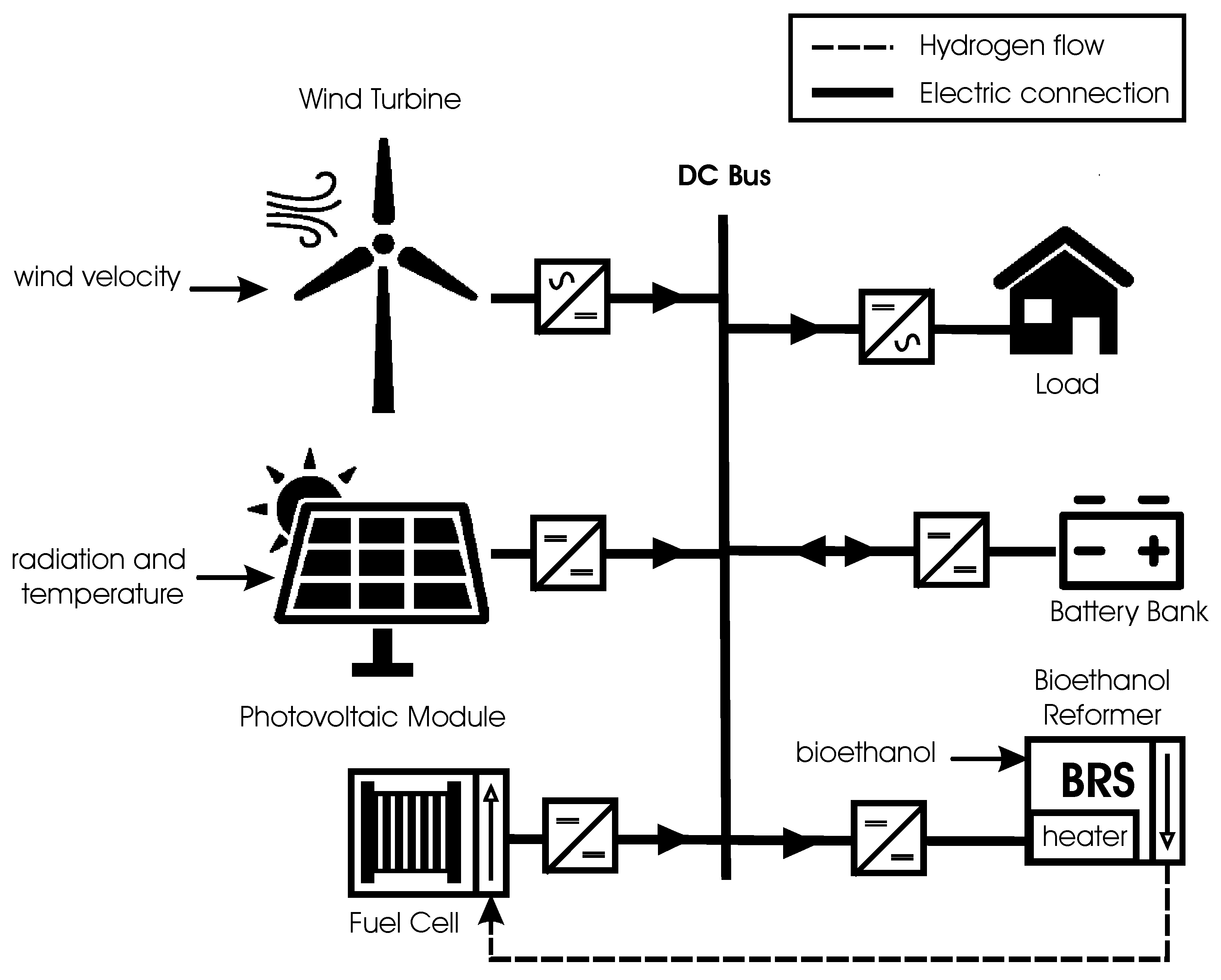
A complete model of the system was implemented in MATLAB/Simulink according to the description of the models of Section 2. The system specifications, $SoC$ levels, the constant battery charging power, as well as maximum power adopted are shown in

Table 6. Real system specifications and EMS parameters.

Parameter	Variable	Value
System Specifications
Autonomy time	$T_{auto}$	3 h
Recharge time	$T_{ch}$	6 h
SoC Levels and Pch calculation
Minimum $SoC$ value	$So{C}_{min}$	$0.4$
Maximum $SoC$ value	$So{C}_{max}$	$0.9$
$SoC$ Level 1	$So{C}_{L1}$	$0.71$
Maximum load power	$P_{load}^{max}$	$4100\mathrm{W}$
Maximum fuel cell power	$P_{fc}^{max}$	$4800\mathrm{W}$
Maximum power required by the heater	$P_h^{max}$	$1553\mathrm{W}$
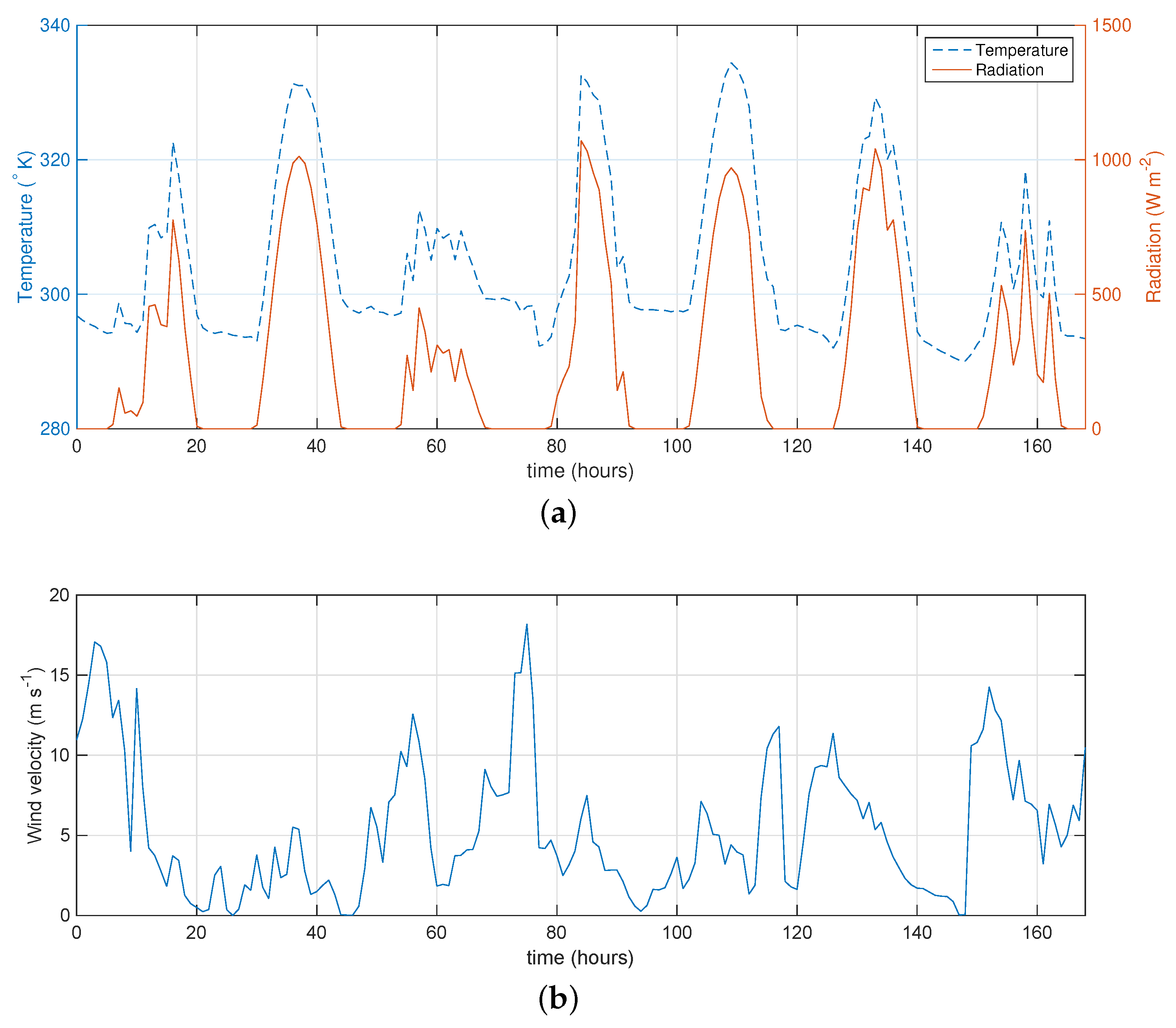
Batteries charging power	$P_{ch}$	$426\mathrm{W}$

. The profiles corresponding to the generation from RESs and the load demand shown in Figure 4 are used to carry out the simulation of the EMS performance.

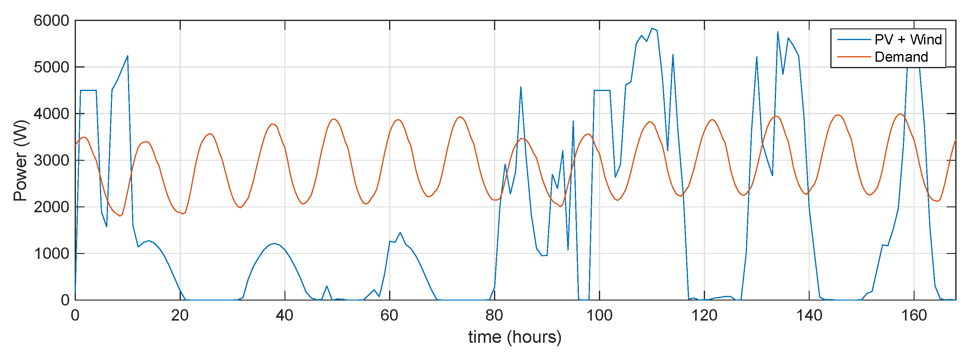
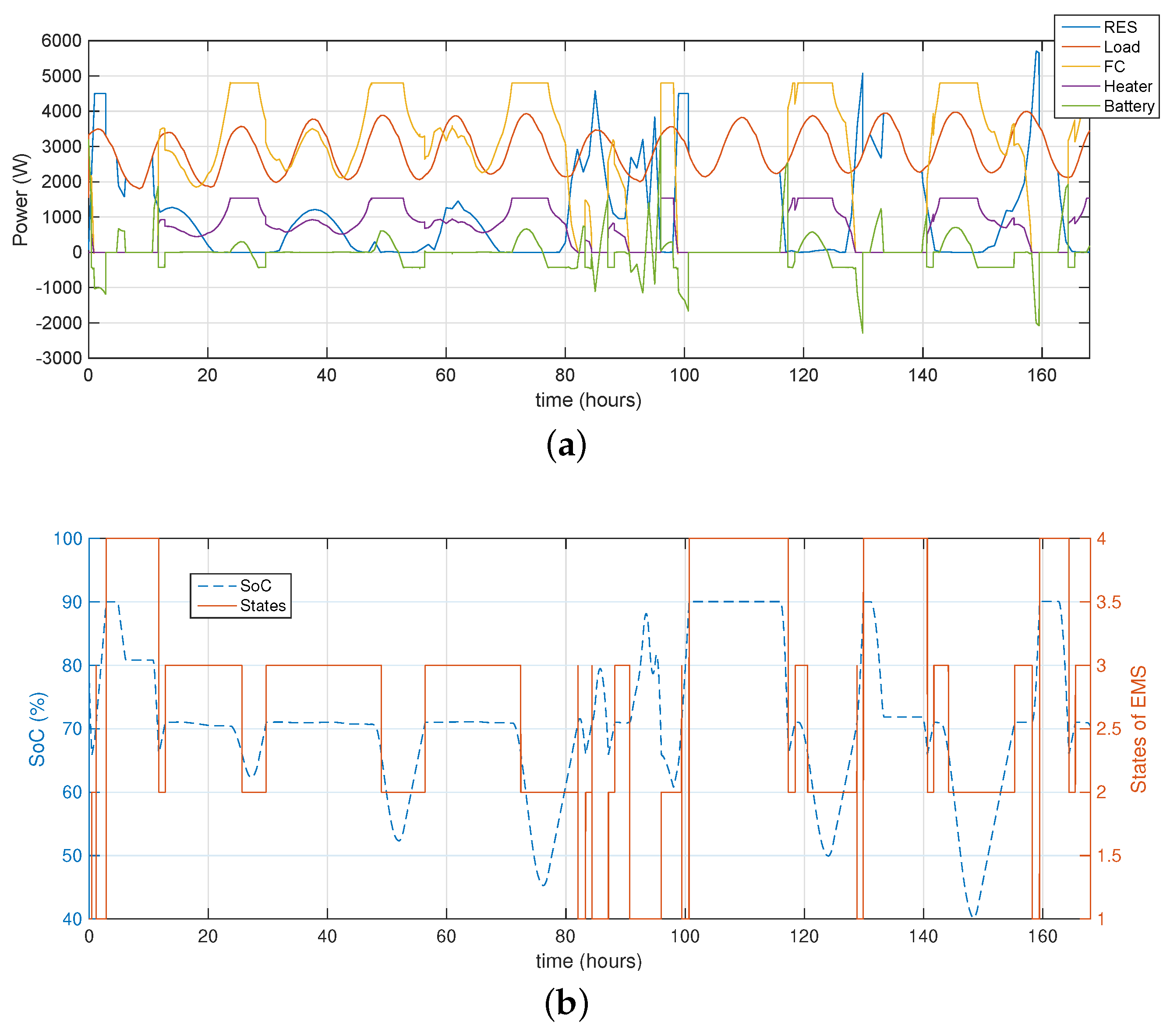
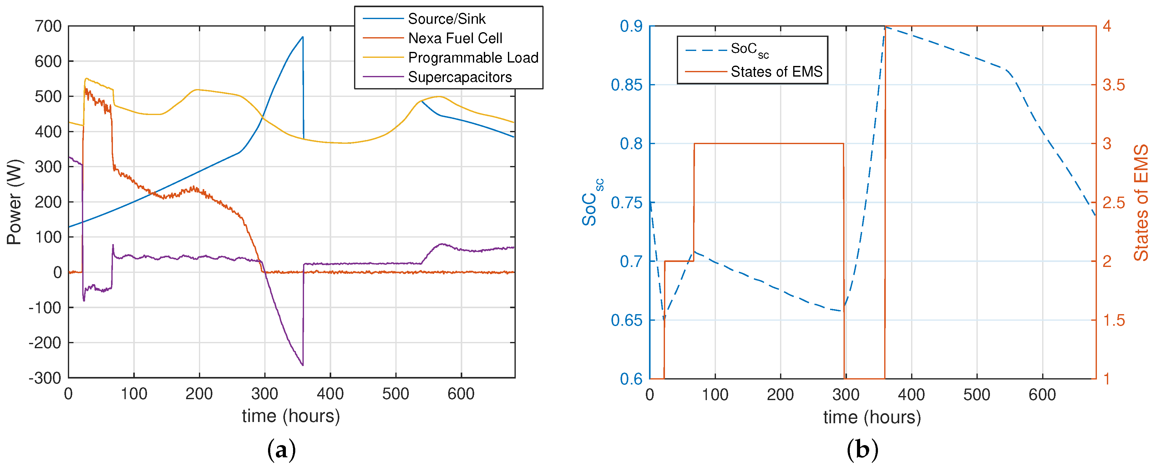
Figure 5a shows the resulting power distribution on the HRES. As can be seen, the specifications stated in Section 3 are satisfied by applying the proposed EMS. The RESs work in MPPT most of the time, and the batteries are charged if the generation from RESs exceeds the load demand, until $So{C}_{max}$ is reached. At this point, the RES goes to work in LPT mode (e.g., between Hour 100 and 116). The PEMFC acts as a secondary source when the RESs produce less than the load demand, while the batteries ensure the power balance during transient periods. 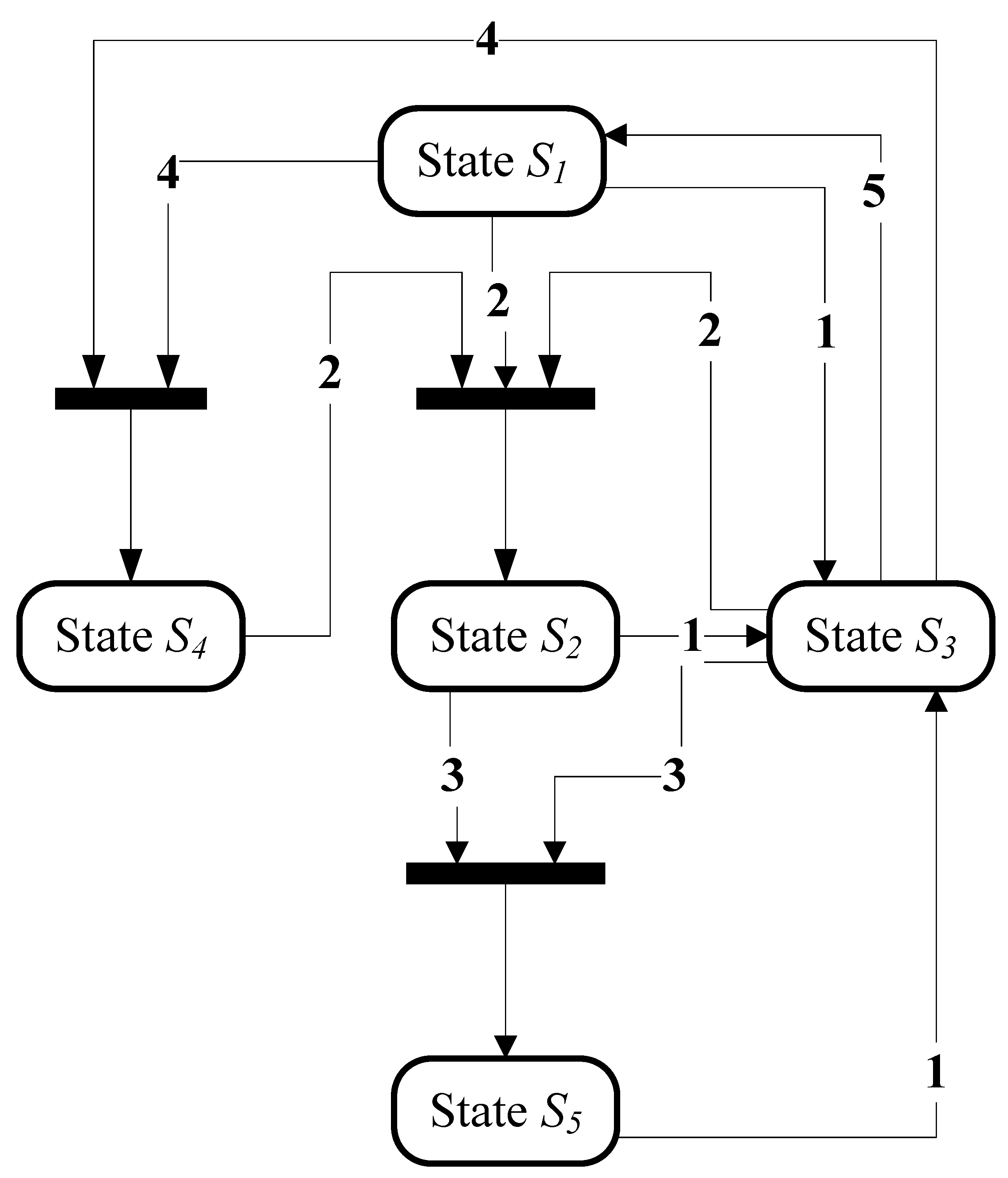Figure 5b shows the behavior of the $SoC$ and the states in which the EMS works. It can be seen that the EMS ensures the power balance, trying to keep the $SoC$ at the desired value ($So{C}_{L1}$). This value is between $So{C}_{min}$ and $So{C}_{max}$, giving the battery the ability to absorb or deliver energy if there is an excess or lack of power in the DC bus, respectively. Finally, it can be mentioned that the simulation results obtained have demonstrated the ability of the EMS to manage the energy in the system.

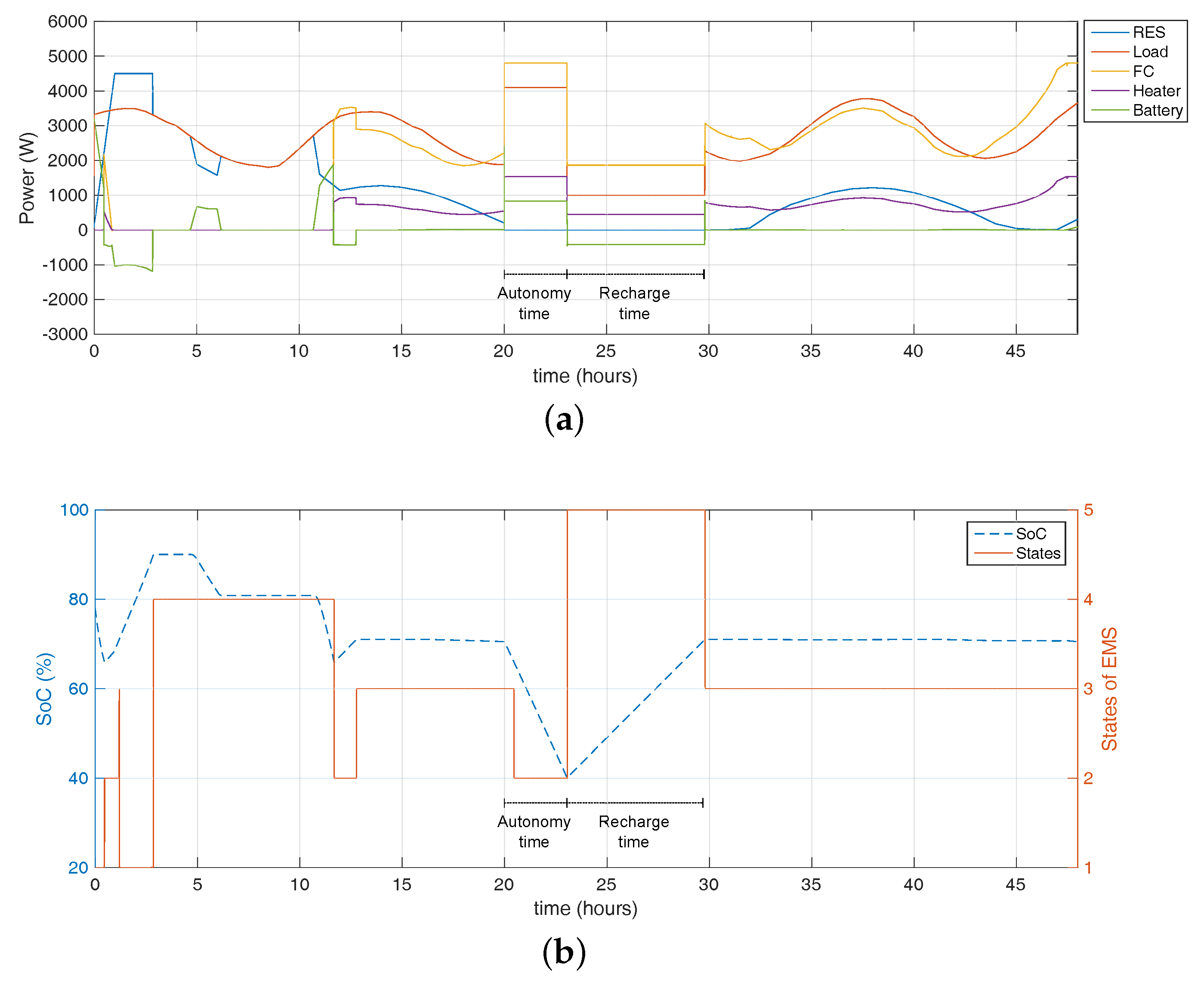
It is necessary to evaluate the performance of the EMS and verify the compliance with the system specifications (autonomy time and recharge time) in a critical scenario. Figure 6a shows the power distribution in the simulated scenario, while Figure 6b shows the corresponding $SoC$ evolution and states of the EMS. At time $t=20\mathrm{h}$, the generation from the renewable sources is set to zero, and the load demand is set to its rated value. As a result of this, the fuel cell and the battery feed the load demand, and the battery is discharged during the autonomy time from $So{C}_{L1}$ to $So{C}_{min}$. At this moment, the EMS changes from State 2 to State 5, where only the vital loads are fed. Then, batteries start to charge (recharge time) until the $So{C}_{L1}$ is reached, and the EMS leaves State 5. At this point ($t=30\mathrm{h}$), the critical scenario is reset, and the normal conditions are restored. The simulations show an adequate fulfillment of the imposed specifications.

4.3. Laboratory Station Description

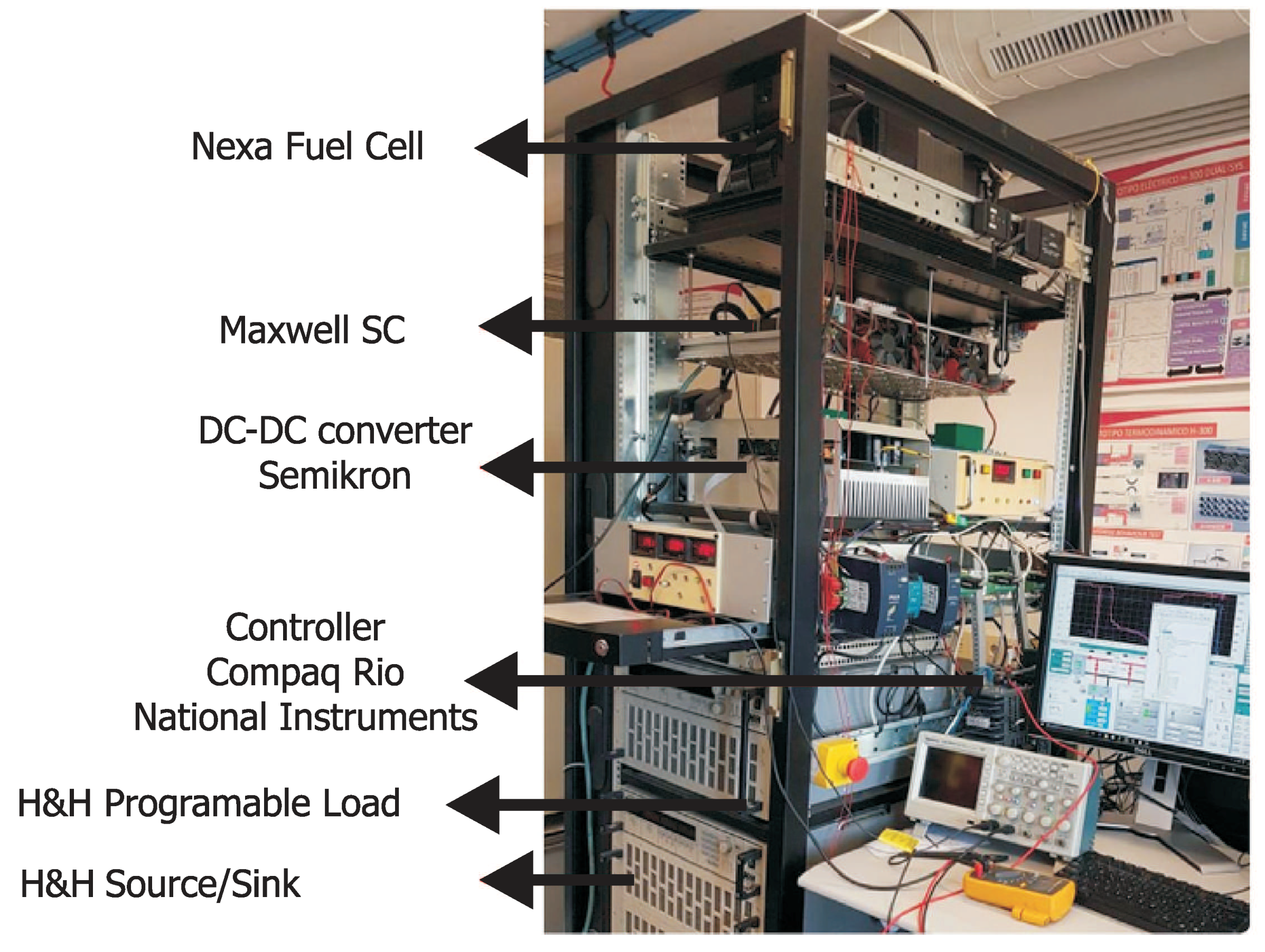
The experimental validation was performed in the Fuel Cell Laboratory of the Institut de Robòtica i Informàtica Industrial (IRI) of the Technical University of Catalonia (CSIC-UPC), in Barcelona, Spain. In this work, a fuel cell test station is used, which consists of a PEMFC stack and a supercapacitor (SC) bank. The SC is used in this experimental setup to replace the batteries as the energy storage. The demand profile is emulated by a programmable load, while the RESs generation is emulated with a programmable current source/sink. A picture of the laboratory station is shown in Figure 7. This station has already been used successfully to validate an EMS applied to hybrid vehicle in [30].

The PEMFC stack is a $1.2\mathrm{kW}$ Nexa^TM model MAN5100078, manufactured by Ballard^TM. The output voltage can be operated safely in the linear range of voltages from $26\mathrm{V}$ to $36\mathrm{V}$ and currents from $10\mathrm{A}$ to $46\mathrm{A}$. The ESS consists on a $165\mathrm{F}$ Maxwell^TM Supercapacitor model BMOD0165. The nominal voltage is $48\mathrm{V}$ with values up to a maximum of $52\mathrm{V}$. The SC supports a nominal current of 98 in continuous mode and shows a serial resistance of approximately $6\mathrm{m}$. The DC-DC boost converters are implemented with two branches of Semikron^TM IGBTs. The converters are controlled with a $20\mathrm{kHz}$ PWM signal, whose switching duty cycle is set by the EMS. The maximum voltage allowed in each switch is $400\mathrm{V}$, and the nominal current is $75\mathrm{A}$. The inductances in the converters have a value of $35\mathsf{\mu }\mathrm{Hy}$. The DC bus voltage adopted is $75\mathrm{V}$, and the bus capacitance is $2720\mathsf{\mu }\mathrm{F}$. The programmable source is an NL Source-Sink (SS) from Hocherl & Hackl GmbH^TM. The output voltage of this source can reach a maximum of $80\mathrm{V}$ with a nominal power of $3.2\mathrm{kW}$. The installed programmable load (PL) is a ZL Electronic DC Load from Hocherl & Hackl GmbH^TM, which can work with a maximum voltage of $80\mathrm{V}$ and $3.4\mathrm{kW}$. Finally, the control is implemented using a National Instruments^TM controller model Compaq Rio 9035, which has a CPU Dual-Core of $1.33\mathrm{GHz}$ and an FPGA Xilinx Kintex-7 7K70T. The rated values of the fuel cell test station are summarized in

Table 7. Fuel cell test station rated values.

Parameter	Variable	Value
H&HTM SSmaximum power	$P_{max}^{ps}$	$3200\mathrm{W}$
H&HTM PLmaximum power	$P_{max}^{pl}$	$1600\mathrm{W}$
NexaTM maximum power	$P_{fc,max}^s$	$1200\mathrm{W}$
NexaTM maximum raising rate power	$\Delta P_{fc,max}^s$	$120\mathrm{W}/\mathrm{s}$
MaxwellTM SC maximum current	$I_{sc}^{max}$	$40\mathrm{A}$

.

4.4. Scaling Methodology

In this work, a method is developed to scale a given scenario so that it can be reproduced in the test station. The scaling methodology preserves most of the relevant energy-flow characteristics. Henceforward, the term scaled (superscript s) will be used to refer to the test station, while the term real (superscript r) to the HRES described in Section 2 together with the realistic scenario.

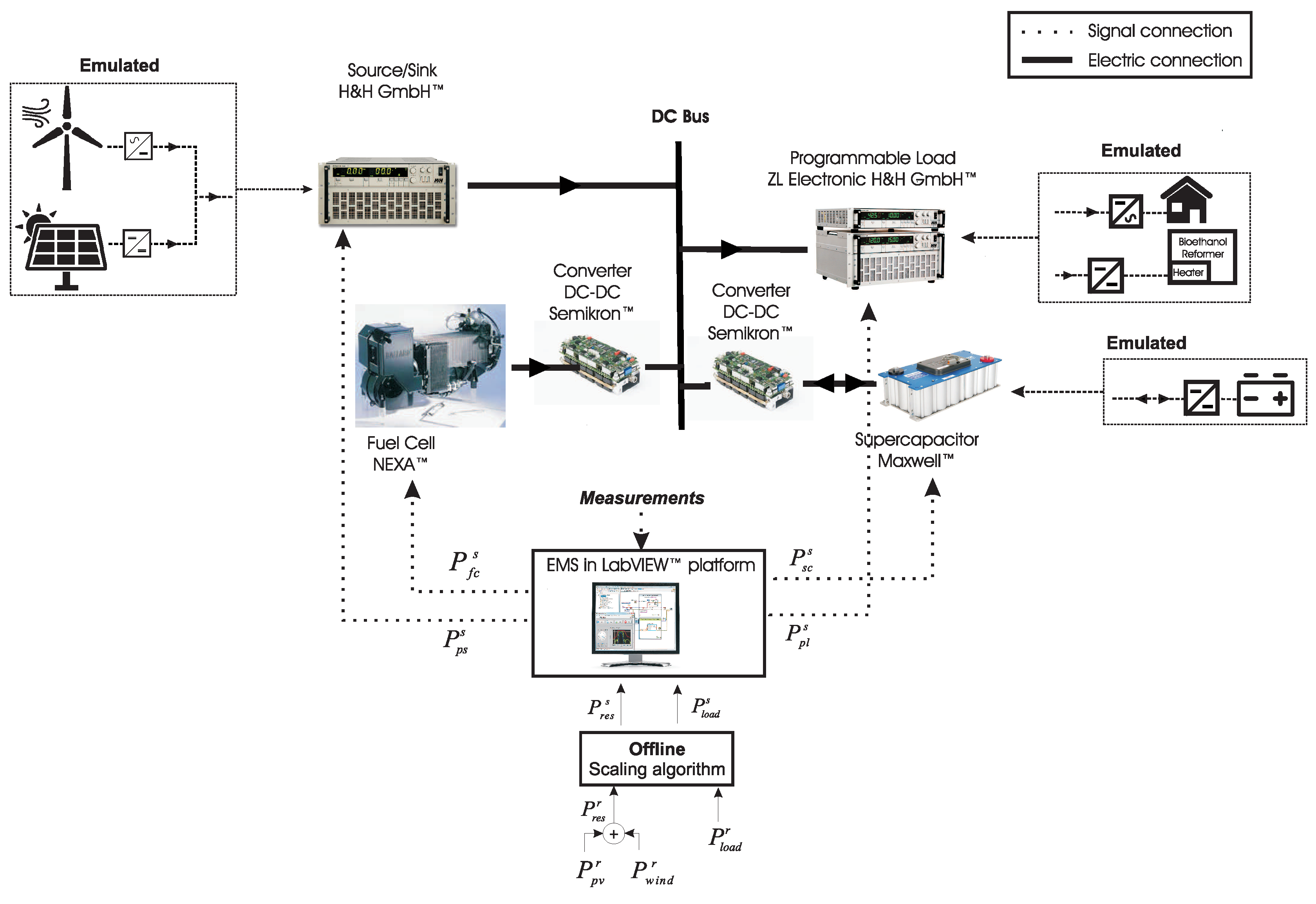
Figure 8 shows the experimental setup used. The EMS is executed in a host computer running a LABView^TM platform. The PEMFC stack and the SCs are connected to the DC bus through DC-DC converters. The H&H Source/Sink is used to emulate the RES generation delivered to the bus ($P_{ps}^s$). The scaled version of RES’s available power ($P_{res}^s$) is obtained using the off-line scaling methodology applied to the real RES generation profile ($P_{res}^r$), which is formed by the wind turbines’ ($P_{wind}^r$) and PV array’s ($P_{pv}^r$) available powers. The scaled version of the load demand ($P_{load}^s$) and the power consumed by the BRS heater ($P_h^s$) are emulated using the programmable load ($P_{pl}^s$). Note that the energy required by the heater is obtained using the power delivered by the Nexa^TM.

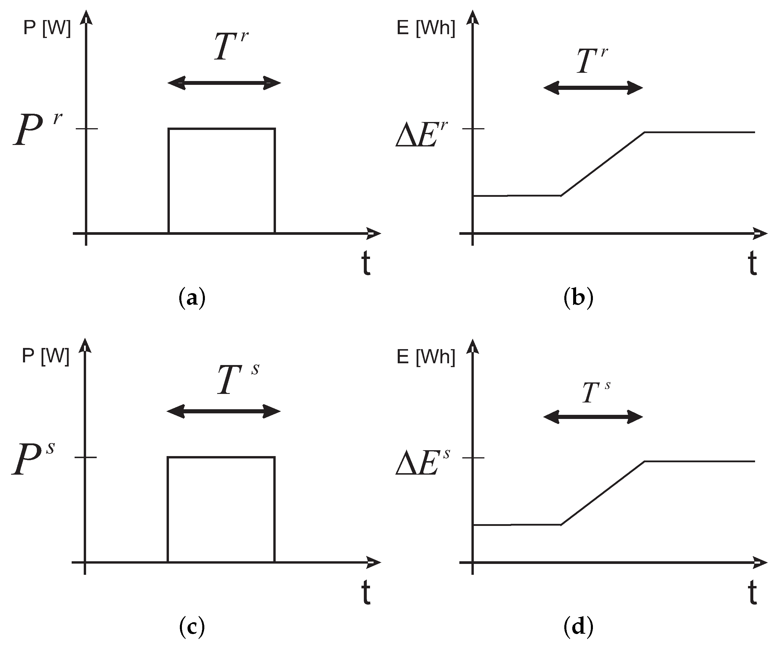
Given a real system with a net power $P^r$ during a period $T^r$ (Figure 9a), the stored energy results $\Delta E^r=P^r{T}^r$ (Figure 9b). In the same way, in the laboratory test station, there is an equivalent scenario with a power $P^s$ and time $T^s$ (Figure 9c), resulting in a stored energy $\Delta E^s$ (Figure 9d). The relative change with respect to the maximum energy capacity $E_{max}^i$ (with $i=r,s$) can be expressed as:

$$\frac{\Delta E^i}{E_{max}^i}=\frac{P^i{T}^i}{E_{max}^i}.$$

(38)

The relationship between the real scenario and the scaled scenario can be defined taking into account that the power step must produce the same relative change in the stored energy of both scenarios. From Equation (38), it results:

$$\frac{E_{max}^s}{E_{max}^r}=\frac{P^s{T}^s}{P^r{T}^r}.$$

(39)

The scaling coefficients can be defined by Equation (39):

$$\begin{array}{ccc}\hfill k_e& =& \frac{E_{max}^r}{E_{max}^r},\hfill \end{array}$$

(40)

$$\begin{array}{ccc}\hfill k_p& =& \frac{P^s}{P^r},\hfill \end{array}$$

(41)

$$\begin{array}{ccc}\hfill k_t& =& \frac{T^s}{T^r},\hfill \end{array}$$

(42)

while the fundamental relationship can be rewritten as:

$$k_e=k_p{k}_t,$$

(43)

where $k_e$, $k_p$ and $k_t$ are the energy, power and time scaling coefficients, respectively. Then, the load and RES scaled profiles result:

$$\begin{array}{ccc}{P}_{res}^s\hfill & =\hfill & k_p\left(P_{wind}^r+P_{pv}^r\right),\hfill \\ P_{load}^s\hfill & =\hfill & k_p{P}_{load}^r+P_h^s.\hfill \end{array}$$

(44)

Note that the power consumed by the heater in the scaled system ($P_h^s$) is not multiplied by $k_p$ because it is calculated by Equation (1) using the measure of the power delivered by the fuel cell ($P_{fc}^s$).

As described in Section 2.5, the ESS in the real system is formed by a battery bank. Then, the maximum energy storing capacity ($E_{max}^r$) can be approximated by:

$$E_{max}^r\approx C_{bat}{V}_{bat}^r.$$

(45)

Since the ESS in the test station is composed of SCs, the maximum energy storing capacity ($E_{max}^s$) is calculated as:

$$E_{max}^s=\frac{1}{2}{C}^{sc}[{\left(V_{max}^{sc}\right)}^2-{\left(V_{min}^{sc}\right)}^2],$$

(46)

where $C^{sc}$ is the capacity of the SC and $V_{max}^{sc}$ and $V_{min}^{sc}$ are the maximum and minimum voltage imposed on the SC in the emulation test, respectively. Note that the definition of a minimum and a maximum value in the SC voltage allows us to manipulate its energy capacity, which is one of the scaling process variables. The $So{C}_{sc}$ level from the SC can be calculated as:

$$So{C}_{sc}\left(k\right)=1-\frac{{\left(V_{max}^{sc}\right)}^2-{\left(V^{sc}\left(k\right)\right)}^2}{{\left(V_{max}^{sc}\right)}^2-{\left(V_{min}^{sc}\right)}^2},$$

(47)

where $V^{sc}\left(k\right)$ is the SC voltage.

Then, replacing (40), (45) and (46) in (43), the power scaling coefficient results:

$$k_p=\frac{\left(\frac{\frac{1}{2}{C}^{sc}[{\left(V_{max}^{sc}\right)}^2-{\left(V_{min}^{sc}\right)}^2]}{C_{bat}{V}_{bat}^r}\right)}{k_t}.$$

(48)

To avoid exceeding the laboratory station capacities established in Section 4.3 and taking into account the case study description, some constraints must be imposed on Equation (48). The power scaling coefficient ($k_p$) must take into account the power range of the real system profiles (RESs, load demand and fuel cell) in such a way that the scaled powers do not exceed power equipment limitations. These constraints impose upper bounds on $k_p$:

$$\begin{array}{ccc}\hfill k_{p_{ub1}}& =& \frac{P_{max}^{ps}}{P_{res,max}^r},\hfill \end{array}$$

(49)

$$\begin{array}{ccc}\hfill k_{p_{ub2}}& =& \frac{P_{max}^{pl}}{P_{load,max}^r+P_{h,max}^r},\hfill \end{array}$$

(50)

$$\begin{array}{ccc}\hfill k_{p_{ub3}}& =& \frac{P_{fc,max}^s}{P_{fc,max}^r},\hfill \end{array}$$

(51)

where $P_{max}^{ps}$ is the rated power of the source/sink and $P_{max}^{pl}$ is the rated power of the programmable load. $P_{res,max}^r$ is the maximum power peak of the RES generation profile; $P_{load,max}^r$ is maximum load demand; and $P_{h,max}^r$ is the power consumed by the electric heater with the fuel cell at its maximum power. $P_{fc,max}^r$ is the rated power of the fuel cell in the real scenario, while $P_{fc,max}^r$ is the rated power of the Nexa^TM fuel cell.

In addition, the maximum current of the SC ($I_{max}^{sc}$) also imposes an upper bound on $k_p$. In charging mode, the maximum current occurs with the maximum charging power and the minimum voltage. With the proposed EMS, the maximum charging power matches the maximum RES generated power ($P_{res,max}^r$), while the minimum voltage is $V_{SoC,min}^{sc}$:

$$k_{p_{ub4}}=\frac{I_{max}^{sc}{V}_{SoC,min}^{sc}}{P_{res,max}^r}.$$

(52)

In discharging mode, the maximum power is when the SC has to provide all the power required by the load:

$$k_{p_{ub5}}=\frac{I_{max}^{sc}{V}_{SoC,min}^{sc}}{P_{load,max}^r}.$$

(53)

It is expected that the maximum power rate allowed in the laboratory station fuel cell ($\Delta P_{fc,max}^s$), once unscaled, would not exceed the real system constraints ($\Delta P_{fc,max}^r$):

$$\Delta P_{fc,max}^s\left({\displaystyle \frac{k_t}{k_p}}\right)\le \Delta P_{fc,max}^r.$$

(54)

This constraint imposes a lower bound on $k_p$ that depends on $k_t$:

$$k_{p_{lb}}=\left(\frac{\Delta P_{fc,max}^s}{\Delta P_{fc,max}^r}\right)k_t.$$

(55)

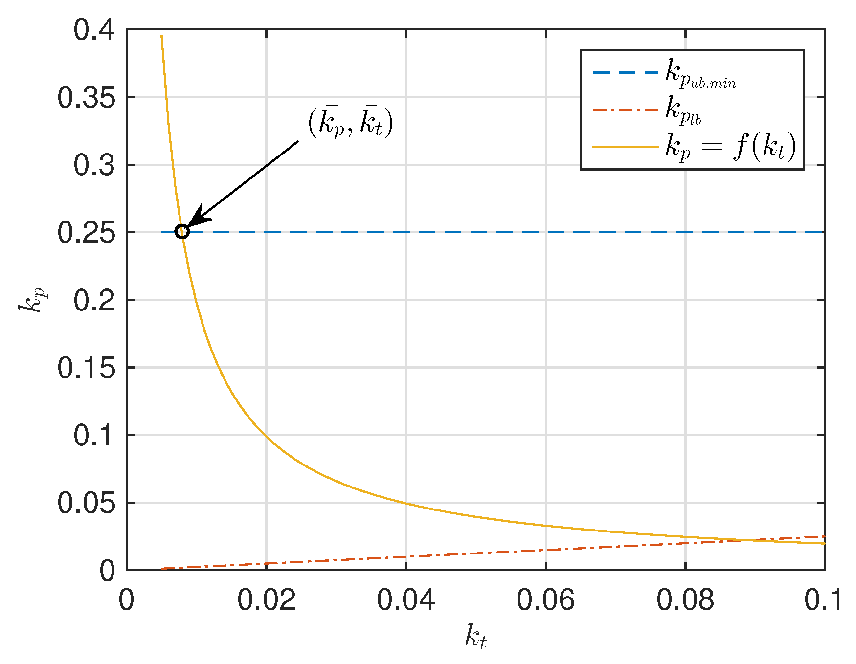
In Figure 10 are summarized the feasible values of the scaling coefficients ($k_p,k_t$) and the constraints described before. As can be seen, $k_p$ can take values in the dashed line (defined by Equation (48)) between the lower bound ($k_{p_{lb}}$) and the most restrictive upper bound ($k_{p_{ub,min}}$). To obtain an experimental test duration as short as possible, a value of $k_t$ as small as possible has to be chosen. Then, the adopted scaling coefficient pair $(\overline{k_p},\overline{k_t})$ is in the intersection defined by Equation (48) and $k_{p_{ub,min}}$. Finally,

Table 8. Experimental validation data and parameters of the scaling methodology.

Parameter	Variable	Value
Real System
Maximum Battery energy storing capacity	$E_{max}^r$	$8112\mathrm{Wh}$
Fuel cell nominal power	$P_{fc,max}^r$	$4800\mathrm{W}$
Fuel Cell maximum raising rate power	$\Delta P_{fc,max}^r$	$480\mathrm{W}/\mathrm{s}$
Heater power at fuel cell nominal power	$P_{h,max}^r$	$1553\mathrm{W}$
Maximum load power	$P_{load,max}^r$	$4100\mathrm{W}$
Maximum renewable energy source power	$P_{res,max}^r$	$5000\mathrm{W}$
Laboratory station: SC voltage values
MaxwellTM SC maximum voltage	$V_{max}^{sc}$	$40\mathrm{V}$
MaxwellTM SC minimum voltage	$V_{min}^{sc}$	$30\mathrm{V}$
MaxwellTM SC voltage at $So{C}_{min}$	$V_{SoC,min}^{sc}$	$34.3\mathrm{V}$
Scaling Coefficients
Power coefficient	$\overline{k_p}$	$0.25$
Time coefficient	$\overline{k_t}$	$0.0079$
Energy coefficient	$\overline{k_e}$	$0.0020$

summarizes the characteristic values of the real scenario, the adopted voltage values for the SCs in the emulation test and the resulting scaling coefficients. The values of the maximum RES generation and the maximum load demand were obtained from the real scenario taking into account a complete year.

4.5. Experimental Results

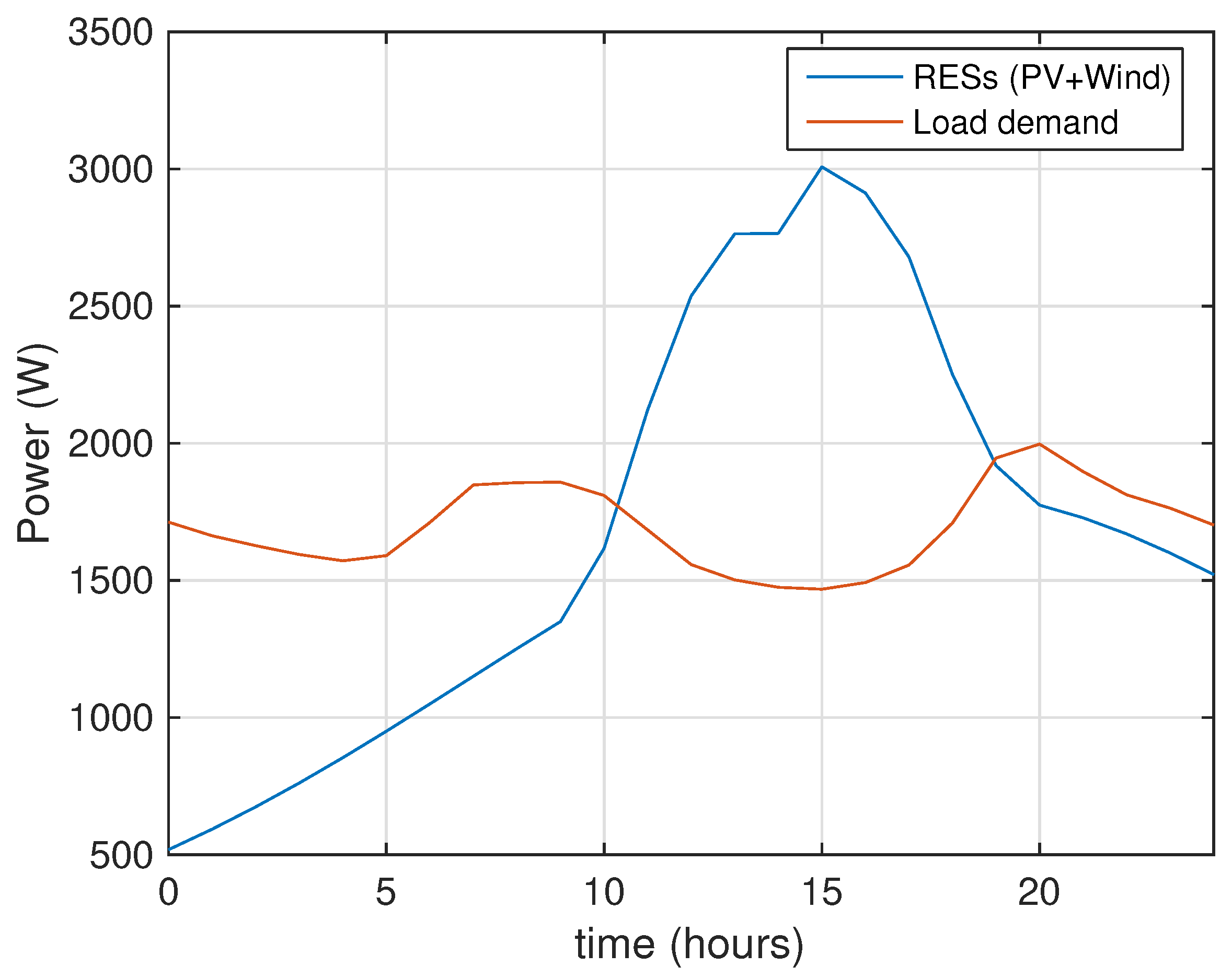
The experimental validation of the EMS was performed using a typical winter day from the annual profiles of the real scenario. Figure 11 shows the evolution of power generation from renewable sources (blue line) and the load power demanded (red line) over the selected day. With regard to the power generated, this power is the sum of the powers corresponding to the two renewable sources: wind and photovoltaic. This power has a peak at 15 o’clockdue to the contribution of sun and wind and a valley during the night because there is no contribution from the Sun. With regard to the curve of the power demanded, it is a profile consistent with the power demand of a home where two peaks are observed, one in the morning near noon and another near dinner time, and two valleys, one in the morning and the other in the afternoon.

Then, the power profiles were scaled according to the methodology presented in Section 4.4 to perform the experimental test. Note that, once scaled, the original length of 24 × 3600 = 86,400 s resulted in a duration of the experiment of 86,400 $\times k_t$ = 682.5 s. The reduction in experiment duration is an important advantage that results from applying the proposed scaling methodology.

Figure 12a shows the power distribution resulting from the test. As explained in Section 4.3, the RES generation is emulated with the source/sink, while the load demand and the power consumed by the heater are emulated with the programmable load. Note that, while the load demand is scaled from the load profile of Figure 11, the power required by the heater is obtained from Equation (1) using the measured power of the Nexa^TM fuel cell. The power delivered by the fuel cell is set by the EMS, and the power delivered/absorbed by the SC arises as a result of the two PI controllers in cascade that attempt to maintain the DC bus voltage at the desired level, while in the simulation, it is computed from a power balance. A constant power delivered by the SC can be seen that corresponds to the necessary power to maintain the DC bus at the desired value. Then, Figure 12b shows the evolution of the state of charge of the batteries and the state in which the EMS works. The commutations between states according to the occurrence of events can be seen.

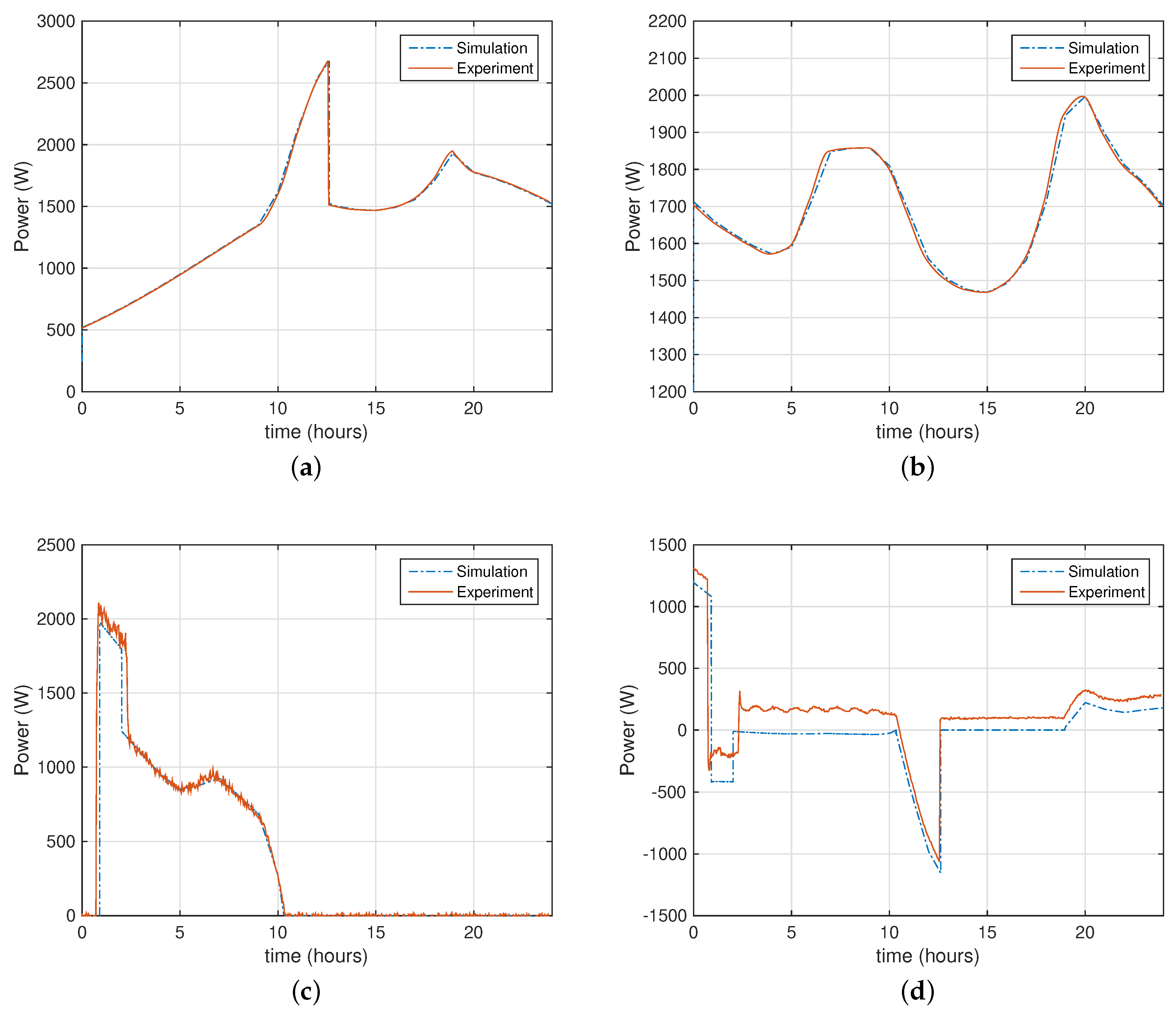
The HRES behavior is simulated using the profiles of Figure 11 and compared with the experiment results. The inverse scaling process is carried out over the profiles presented in Figure 12a. The evolutions of the main variables, both in simulation and in the experimental test, are shown in Figure 13. The RES generation and the load power demand, which are emulated with the source/sink, and the programmable load are shown in Figure 13a,b. In Figure 13c is shown the Nexa^TM fuel cell, where the main difference of the experiment evolution with respect to the simulation is a small noise. The major differences observed between experimental and simulation results are found in the SC power of Figure 13d and are due to the low efficiency in the bidirectional DC-DC converter, especially at low powers. This could be solved by incorporating the models of the converters with their efficiency curves. This improvement will be addressed in future works.

In summary, the experimental results presented in this section have demonstrated the feasibility of implementing the proposed EMS for the HRES under study. In the same way, the proposed scaling methodology provides a useful tool to evaluate the qualitative behavior of the main HRES variables in a real scenario.

5. Conclusions

This paper describes an energy management system for an isolated hybrid renewable energy system. In this sense, a comprehensive and innovative approach was presented and validated. The EMS proposed is based on a finite state machine designed to obtain good performance in the autonomy and recharge time. The performance of the EMS has been evaluated using historic profiles representing different weather and load conditions; firstly, running the simulation using a MATLAB/Simulink complete model and later in a scaled experimental laboratory setup. In both cases, the EMS offered correct results in terms of compliance with the imposed specifications, and also, the experimental results obtained agree with those obtained by the simulation. As a conclusion, it can be established that the proposed EMS can be implemented easily in real time and offers adequate results. Finally, it is worth mentioning that although the results are focused on a specific HRES, the methodologies presented in this document are general enough to cover a wide range of problems related to energy management in HRES.