Article

Enhancing Arctic Ice Extent Predictions: Leveraging Time Series Analysis and Deep Learning Architectures

1
Department of Mathematics, Bradley University, Peoria, IL 61625, USA
2
Siebel School of Computing and Data Science, University of Illinois Urbana-Champaign, Champaign, IL 61820, USA
3
Computational and Applied Mathematics, FAU Erlangen-Nuremberg, D-91058 Erlangen, Germany
*
Author to whom correspondence should be addressed.
Glacies 2025, 2(4), 12; https://doi.org/10.3390/glacies2040012
Submission received: 19 August 2025 / Revised: 10 October 2025 / Accepted: 14 October 2025 / Published: 30 October 2025

Abstract

With ongoing climate transformations, reliable Arctic sea ice forecasts are essential for understanding impacts on shipping, ecosystems, and climate teleconnections. This research examines physics-free neural architectures versus physics-informed statistical models for long-term Arctic projections by implementing Fourier Neural Operator (FNO) and Convolutional Neural Network (CNN) alongside a seasonal SARIMAX time series model incorporating physical predictors including temperature anomalies and ice thickness. We test whether neural models trained on historical ice data can match physics-informed SARIMAX reliability, and whether approaches exhibit systematic biases toward specific emission pathways. Using data from January 1979 to December 2024, we conducted forecasts through 2100, with SARIMAX driven by CMIP6 sea ice thickness under SSP2-4.5 and SSP5-8.5 scenarios. Results decisively reject the first hypothesis: both neural models projected ice free Arctic summer by September 2089 regardless of emission scenario, while SARIMAX maintained physically plausible seasonal coverage throughout the century under both pathways. Neural approaches demonstrated systematic bias toward extreme warming exceeding even high-emission projections, revealing fundamental limitations in physics-free deep learning for climate forecasting where physical constraints are paramount.

1. Introduction

Over the past thirty years, numerous studies have documented the rapid decline of Arctic sea ice [1,2,3]. This trend is largely driven by the region’s heightened sensitivity to climate change: rising greenhouse gas emissions and ocean heat transport from the Atlantic trigger a positive feedback loop, a self-reinforcing process in which initial warming accelerates further ice loss and additional heat absorption by newly exposed ocean surface [4]. As more ice melts, open ocean absorbs additional heat, accelerating warming in a process known as Arctic amplification, the tendency of the Arctic to warm faster than the global average due to feedback mechanisms (e.g., ice–albedo and lapse–rate feedbacks) [5]. This rapid loss of sea ice has far-reaching effects on mid-latitude climates, economic interests, and ecological stability.
Various studies have provided suggestive evidence linking Arctic sea ice decline to mid-latitude climate anomalies through both tropospheric and stratospheric pathways. A key early study by [6] used a primitive general circulation model to simulate an ice-free Arctic. Notably, the model predicted cooling in mid-latitude regions, although the author acknowledged that these findings were limited by the model’s simplifications. More recent investigations by [7,8] describe similar connections but emphasize that the relationship appears episodic and requires further research for definitive confirmation. Nevertheless, the current body of evidence suggests that Arctic sea ice loss can indeed influence broader climate patterns, underscoring its significance as a driver of global climate variability.
Additionally, the melting of Arctic sea ice has significant economic implications, especially for commercial shipping. The decline in sea ice along the Northern Sea Route (NSR) during summer offers a shorter alternative to traditional shipping passages. A 2017 study estimated that under high emissions, the NSR could eventually handle about 5% of global trade [9] leading Russia, China, and several other countries to invest heavily in developing this corridor [10]. While increased Arctic shipping can boost economic prospects by shortening routes, it also raises serious climate concerns. In response, recent regulations have restricted the use of heavy fuel oil in the Arctic to limit further warming from expanded NSR traffic [10]. This tension between economic opportunity and climate protection will likely remain a source of international debate for decades to come.
Climatological shifts from Arctic sea ice loss have the potential to devastate the region’s ecosystem. Models indicate that shrinking ice will significantly reduce phytoplankton, the main primary producers, likely shifting the food web toward heterotrophy and weakening coastal marine productivity, with observational evidence showing that coastal erosion and changing ice dynamics are already reshaping nearshore planktonic food webs [11]. Ice-dependent species like polar bears are also suffering, as longer ice-free summers strand them on land and cut them off from their primary food sources, leading to documented energetic constraints and altered behavioral strategies during prolonged ice-free periods [12]. The decline of sea ice affects every level of the Arctic ecosystem and could mark a climatological tipping point with far-reaching consequences beyond the region.
Given these severe implications, a central question in climate research has long been when the Arctic will see its first ice-free summer. Early work by Holland et al. [13] showed that abrupt ice loss could bring near-total disappearance as early as 2040, though their simulations were based on relatively coarse-resolution CMIP3 models that underestimated internal variability and were sensitive to initialization conditions. A 2012 study [14] using CMIP3 and CMIP5 models produced an even broader range of projections, with some predicting an ice-free Arctic around 2020 and others not until 2100. This wide spread of predictions revealed significant limitations in the modeling power of CMIP3 and CMIP5, reflecting both structural model biases (overly rapid ice-thickness decline in some models) and scenario differences (assumptions about future emissions and aerosol forcing that diverged from observed trajectories), prompting updates in the more recent CMIP6 projections. The improved CMIP6 ensemble incorporates enhanced sea-ice physics, higher resolution, and updated emissions pathways that better track observed forcing, providing a foundation for more reliable long-term projections when combined with robust statistical frameworks that explicitly account for scenario uncertainty.
More recent work has focused on using statistical and deep learning models to enhance climate-based predictions. For example, Andersson et al. [15] developed IceNet, a probabilistic deep learning system trained with uncertainty quantification, designed for seasonal Arctic ice extent forecasting. With lead times of up to six months, IceNet’s ensemble forecasting framework consistently outperformed dynamical models at seasonal horizons, demonstrating the promise of deep learning for operational, near-term predictions. For longer-term forecasts, Ahanda et al. [16] compared neural networks and seasonal ARIMA models to forecast the timing of an ice-free Arctic summer. While IceNet serves as an important benchmark for seasonal prediction skill, the present study examines whether deep learning architectures can remain viable tools for multi-decadal projections when compared against statistical baselines with exogenous climate ensemble scenarios.
Recent advances have expanded this comparative landscape by explicitly evaluating neural network architectures against both CMIP6-based GCMs and statistical models across diverse polar prediction tasks. Feng et al. [17] demonstrated that ConvLSTM-based architectures outperform CMIP6 models in short-term (10-day) forecasts of Arctic sea-ice concentration, while Ren et al. [18] introduced SICNet_season, a transformer-based model that exceeded the ECMWF SEAS5 dynamical forecast system in predicting September sea-ice extent when initialized in spring. Other innovations include bias correction approaches such as Yuan et al.’s Ice-BCNet [19], which addresses systematic errors in coupled GCM forecasts, and transfer learning methods like Song et al.’s framework [20] that leverages CMIP6 multi-model ensembles to improve pan-Arctic sea-ice thickness predictions. Beyond predictive performance, interpretable machine learning applications have revealed model-specific limitations: Labe and Barnes [21] used neural networks to identify systematic biases in Arctic amplification across climate models, while CNN-based ensemble analyses have disentangled internal variability from forced trends in observed Arctic warming, see also [22]. However, these neural approaches face inherent limitations including dependence on short observational records, risk of overfitting to narrow training windows, and challenges with physical interpretability, particularly at longer horizons under evolving forcing scenarios. These constraints highlight the continued importance of robust statistical models that explicitly incorporate exogenous predictors and maintain transparency in their mechanistic assumptions, providing a critical benchmark against which to evaluate the promise and current limits of machine learning approaches in polar climate prediction.
This study builds on existing research by forecasting long-term Arctic sea ice extent using two neural models: a Fourier Neural Operator (FNO) and a Convolutional Neural Network (CNN). Both methods are well suited to capturing the complex spatiotemporal patterns in sea ice data. Their performance was compared to a benchmark SARIMAX model incorporating exogenous variables such as sea ice thickness and temperature anomalies. Specifically, we test two central hypotheses: first, that Fourier Neural Operator (FNO) and Convolutional Neural Network (CNN) architectures, trained solely on historical sea-ice extent data without explicit physical predictors, can achieve projection performance comparable to a robust statistical model (SARIMAX) that incorporates physical exogenous variables (sea-ice thickness and temperature anomalies). Second, that neural models exhibit systematic bias toward specific emission scenarios, with their long-term projections aligning more closely with SARIMAX forecasts driven by either moderate (SSP2-4.5) or high-emission (SSP5-8.5) sea ice thickness projections, thereby revealing implicit scenario assumptions embedded in the training data. The goal is not to prove that neural models universally outperform SARIMAX, but rather to evaluate whether physics-free deep learning approaches can match the projection consistency of physics-informed statistical models and to identify potential biases that may influence their climate scenario assumptions. This dual-hypothesis framework addresses fundamental questions about the viability of neural models for long-term forecasting and meaningfully contributes to the literature on the disappearance of Arctic ice extent.
The remainder of this paper is organized as follows. Section 2 describes the Arctic sea ice extent data from NSIDC and associated climate variables, including temperature anomalies and ice thickness data that serve as exogenous predictors. Section 3 presents the methodological framework, covering time series models (SARIMA/SARIMAX) in Section 3.1 and neural architectures (CNN and FNO) in Section 3.2, followed by statistical testing procedures in Section 3.3. Section 4 details the implementation of each modeling approach, including model specification and parameter selection for SARIMAX (Section 4.1.1), CNN architecture and preprocessing (Section 4.1.2), FNO spectral implementation (Section 4.1.3), and long-term forecasting methodology incorporating CMIP6 climate projections (Section 4.2). Section 5 presents comprehensive results, beginning with short-term forecasting performance evaluation across all models (Section 5.1) and extending to long-term climate projections with hypothesis testing and comparative analysis (Section 5.2). Finally, Section 6 synthesizes our findings, discusses practical implications for Arctic logistics and policy, addresses societal and ethical dimensions of ice loss projections, and outlines future research directions for physics-informed neural networks in climate modeling. All technical details pertaining to the analysis in this work are provided in Appendix A, Appendix B and Appendix C.

2. Data

To support our forecasting models, we rely on a comprehensive set of observational and reanalysis datasets capturing the historical variability of Arctic sea ice extent, temperature anomalies, and ice thickness from 1979 to 2024. These data provide the empirical foundation for both statistical and neural network models, and are further complemented by CMIP6 climate projections to assess future scenario-based trends.
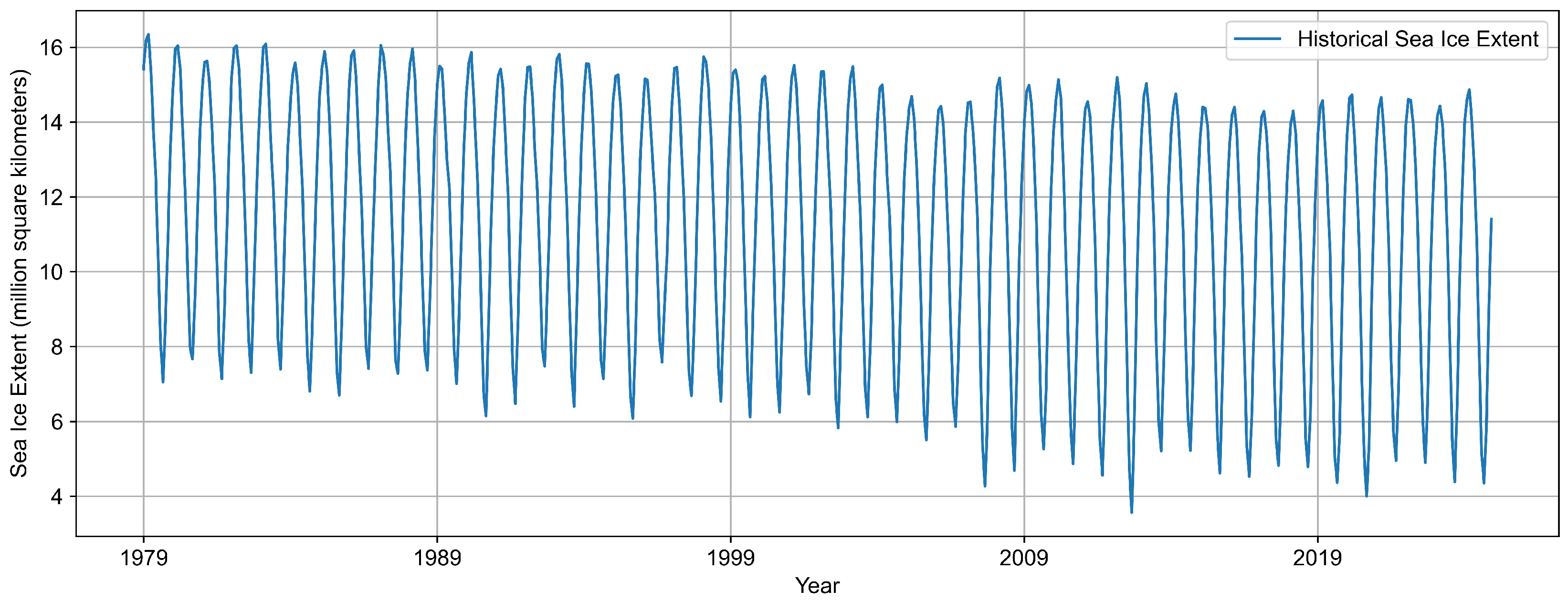
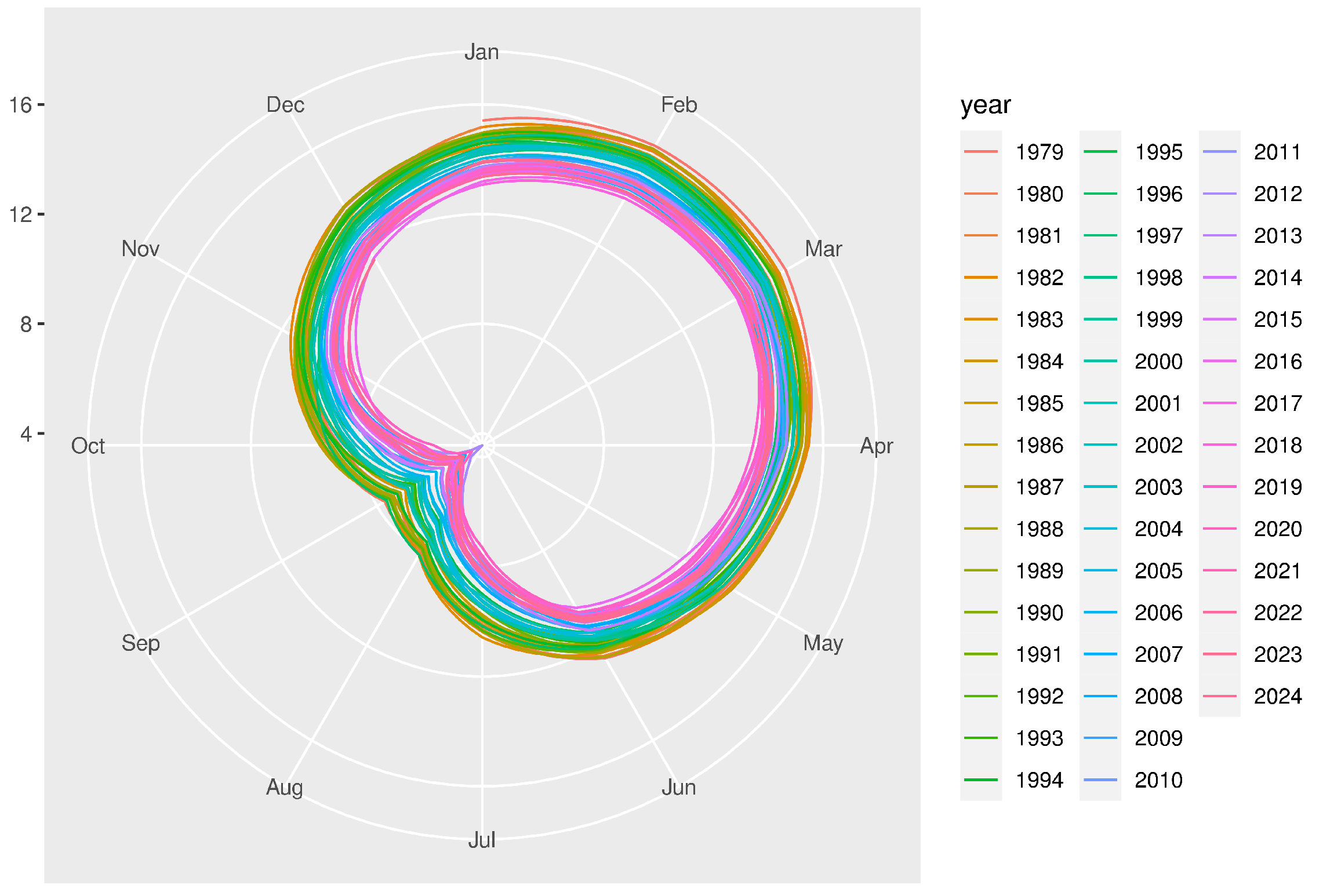
Our modeling is grounded in historical Arctic sea ice data obtained from the National Snow and Ice Data Center (NSIDC), covering the period from 1979 through December 2024. These data from NSIDC are regularly updated and publicly accessible online on [23]. Analysis of satellite data across these years shows strong seasonal variation, typically with a minimum in September and a maximum in March [23] as illustrated in the Arctic ice extent time series in Figure 1 and its polar representation in Figure 2.
It is prudent to note that while the NSIDC dataset represents the most widely used and carefully curated long-term record for Arctic ice extent, our group must acknowledge several known limitations that may affect long-term trend analyses. Over the 1979–2024 record that was used for analysis, NSIDC integrates data from multiple passive microwave sensors, each subject to inter-sensor calibration issues, orbital drift, and algorithm updates, as well as uncertainties introduced by spatial interpolation under cloud cover [24]. These factors can introduce noise into long-term records and have been documented as potential sources of bias in sea-ice trend analyses. However, for our study, which forecasts monthly, pan-Arctic sea-ice extent at multi-decadal timescales, such uncertainties are less likely to affect the large-scale seasonal cycles and interannual-to-decadal variability that form the basis of our modeling framework. Nevertheless, residual biases related to sensor transitions and interpolation remain an important consideration when interpreting long-term projections.
As noted by Ahanda et al. [16], the strong and consistent seasonal patterns observed in Arctic Ice Extent make it well-suited for analysis using time series models such as SARIMAX. In line with their methodology, we applied the SARIMAX model to analyze Arctic Ice Extent, incorporating global monthly temperature anomaly data from NOAA (National Oceanic and Atmospheric Administration) and ice thickness information from the PIOMAS dataset [25] as exogenous regressors. Additional climate indices including the Arctic Oscillation [26] and ENSO (El Niño-Southern Oscillation) [27] from the PIOMAS dataset were initially considered as potential predictors, but preliminary analysis revealed these variables provided no significant predictive power for Arctic Ice Extent and were subsequently excluded from the final model specification.
Supporting the suitability of a SARIMAX-based approach, the linear and curved patterns in the lag plots shown in Figure 3 indicate that the series is autocorrelated, while the pronounced linear pattern at lag 12 confirms the presence of a seasonal cycle repeating every 12 months.
To capture the conditional effect of temperature on Arctic Ice Extent, we incorporated an interaction term between global temperature anomalies and ice thickness into the model. The relationship between these variables is non-additive, thinner ice is more sensitive to warming due to its lower thermal inertia and an amplified ice-albedo feedback. This interaction term accounts for synergistic effects that are not fully captured by the main effects alone, thereby improving the model’s specification and reducing residual variance, as supported by Gerdes [28] and Lang et al. [29]. The time series for global temperature anomalies and Arctic Ice Extent, which form the basis for this analysis, are shown in Figure 4 and Figure 5, respectively.
For long-term forecasting, we used the average CMIP6 climate projections for ice thickness data, as described in [30]. CMIP6 represents the latest coordinated international climate modeling effort, involving over 100 models from 48 institutions across 26 countries and providing the scientific foundation for the IPCC Sixth Assessment Report [31]. The project incorporates significant advances including improved model physics, higher spatial resolutions, and enhanced Earth system components, with standardized output enabling comprehensive analysis across multiple modeling centers.
Figure 3. Lag analysis of the arctic ice extent based on data from January 1979 to December 2024 by courtesy of [23].
Glacies 02 00012 g003
Figure 4. Temperature anomalies series based on data from January 1979 to December 2024 by courtesy of [32].
Glacies 02 00012 g004
Figure 5. Arctic sea ice thickness series based on data from January 1979 to December 2024 by courtesy of [25].
Glacies 02 00012 g005
For long term ice thickness projections in this study, CMIP6 simulations were obtained under two contrasting Shared Socioeconomic Pathways (SSPs). SSP2-4.5 represents a “middle of the road” development pathway with moderate climate policies and technological progress, resulting in intermediate radiative forcing of 4.5   W/m 2 and CO 2 concentrations reaching approximately 543 ppm by 2100. SSP5-8.5 depicts a fossil-fuel intensive future with rapid economic growth and high energy demand, leading to high radiative forcing of 8.5   W/m 2 and CO 2 concentrations exceeding 1135 ppm by century’s end [33]. The inclusion of both scenarios enables assessment of Arctic sea ice thickness evolution under moderate versus high-impact climate futures, capturing the range of uncertainty in emission pathways for robust hybrid forecasting applications through 2100.

3. Methods

Building on this comprehensive, multi-sourced dataset, we adopt a comparative modeling strategy to evaluate distinct approaches for capturing the temporal dynamics of Arctic sea ice extent. The pronounced seasonality, long-term variability, and climate sensitivity of the data motivate systematic comparison between traditional time series models and modern neural model architectures. This comparative framework contrasts the statistical interpretability and physical grounding of conventional approaches against the nonlinear representational capabilities of deep learning methods, enabling assessment of their relative performance for robust, long-range projections through 2100.

3.1. Time Series Models: SARIMA and SARIMAX

For our time series evaluation, we employ SARIMA (Seasonal Autoregressive Integrated Moving Average) and its extended version, SARIMAX (Seasonal Autoregressive Integrated Moving Average with exogenous variables). These models serve as fundamental tools in statistical time series analysis, recognized for their capability to capture intricate temporal dependencies within the data. Let us take a moment to review the time series models employed in this study as well as the models that we pair with it to make long term projections. It should be noted that the R software (version 4.5.1) was utilized for all computations involving the time series models and their exogenous variables, with the exception of the CMIP6 data preprocessing, which was performed using Python (version 3.13.1).

3.1.1. SARIMA Model

SARIMA models excel in managing time series data that display seasonality, along with trends and autocorrelation. This indicates that they can proficiently identify and model recurring patterns that manifest at regular intervals, such as daily, monthly, or yearly cycles. They accomplish this by integrating seasonal components with the non-seasonal autoregressive, integrated, and moving average terms. This widely used approach is known as the ARIMA ( p , d , q ) × ( P , D , Q ) S model. For predicting the average monthly Arctic sea ice extent ( y t ), this model, as detailed by Shumway and Stoffer [34], can be expressed as:
Φ P ( B s ) ϕ ( B ) ( 1 B s ) D ( 1 B ) d y t = Θ Q ( B s ) θ ( B ) w t + δ
where δ is the drift, w t is the standard Gaussian white noise process and
ϕ ( B ) = 1 ϕ 1 B ϕ 2 B 2 ϕ p B p
θ ( B ) = 1 + θ 1 B + θ 2 B 2 + + θ q B q
Φ P ( B s ) = 1 Φ 1 B s Φ 2 B 2 s Φ P B P s
Θ Q ( B s ) = 1 + Θ 1 B s + Θ 2 B 2 s + + Θ Q B Q s
Equations (2) and (3) represent the non-seasonal autoregressive and moving average polynomials of order p and q. Analogously, Equations (4) and (5) denote the seasonal autoregressive and moving average polynomials of order P and Q. Equation (1) demonstrates the dependency of the series y t on its past lags at multiples of the annual seasonal period s. The parameters that must be estimated for this model are ϕ i (non-seasonal autoregressive coefficients) i = 1 , 2 , , p , θ j (non-seasonal moving average coefficients) j = 1 , 2 , , q , Φ k (seasonal autoregressive coefficients) k = 1 , 2 , , P , and Θ l (seasonal moving average coefficients) l = 1 , 2 , , Q , and B is the backshift operator, representing time lags.

3.1.2. SARIMAX Model

SARIMAX enhances the SARIMA framework by permitting the inclusion of exogenous variables. These external factors, which are not part of the primary time series being predicted, can significantly affect its behavior. By integrating such external regressors, SARIMAX can yield more precise forecasts, particularly when the series is influenced by other measurable phenomena. These models provide interpretability, enabling us to comprehend the impact of various components and external factors on the dynamics of the series. For the average monthly extent of Arctic sea ice ( y t ), and with the global temperature anomaly at time t ( h t ), and arctic ice extent thickness at time t ( x t ), and interaction term at time t ( i t ) serving as the regressors, the SARIMAX model is mathematically expressed by Equation (6) below:
Φ P ( B s ) ϕ ( B ) ( 1 B s ) D ( 1 B ) d y t = Θ Q ( B s ) θ ( B ) w t + β 1 x t + β 2 h t + β 3 i t + δ .
The model parameters are estimated using Maximum Likelihood Estimation (MLE), assuming linearity in the relationship between the dependent variable and the exogenous predictors. Standard SARIMAX assumptions are also applied, including the independence and normality of residuals.

3.1.3. Generalized Additive Mixed Models

Generalized Additive Mixed Models (GAMMs) represent an extension of generalized linear mixed models that allow for flexible modeling of nonlinear relationships through the incorporation of smooth functions alongside conventional parametric terms [35]. GAMMs combine the flexibility of generalized additive models (GAMs) with the ability to account for random effects in mixed-effect models, using penalized regression splines to approximate complex nonlinear relationships while estimating their degree of smoothness directly from the data. The framework employs penalized regression splines as basis functions, where smooth terms are constructed from sums of simpler basis functions with associated wiggliness penalties to avoid overfitting, allowing for relatively large basis dimensions while letting the penalty remove excess flexibility. The general GAMM formulation can be expressed as
g ( E [ Y ] ) = X β + f 1 ( x 1 ) + f 2 ( x 2 ) + + f p ( x p ) + Z u ,
where g ( · ) is the link function, X β represents parametric terms, f j ( x j ) are smooth functions of covariates, and Z u captures random effects with u N ( 0 , G ) .
For temperature anomaly extrapolation, the specific GAMM implementation employed penalized regression splines of time with basis dimensions scaled to training sample sizes (up to 60 for fixed windows, 30 for rolling hindcast windows) to capture long-term nonlinear climate trends. The model incorporated ARMA(1,1) residual structures to address temporal autocorrelation in the climate time series, following the formulation: Y t = s ( t , k ) + ϵ t , where s ( t , k ) represents the penalized spline smooth of time with basis dimension k, and ϵ t follows an autoregressive moving average process ϵ t = ϕ ϵ t 1 + θ u t 1 + u t with u t N ( 0 , σ 2 ) . Smoothing parameter selection was performed via restricted maximum likelihood (REML) estimation, which treats the penalized spline as a mixed model where perfectly smooth basis functions become fixed effects and wiggly components are treated as random effects with variance inversely related to the smoothing parameter. This approach allows automatic determination of the optimal balance between model fit and smoothness without requiring a priori specification of knot locations or polynomial degrees, making it particularly suitable for extrapolating complex climate signals to 2100 while maintaining statistical rigor and avoiding overfitting to short-term fluctuations.

3.2. Neural Models: FNO and CNN

Complementing the statistical models, we also investigate the capabilities of contemporary neural models: Fourier Neural Operators (FNO) and Convolutional Neural Networks (CNN). These models signify a shift from conventional statistical methods, providing powerful tools for learning intricate, non-linear relationships directly from data. The Fourier Transform fundamentally offers a comprehensive perspective of the input, enabling FNOs to more efficiently capture long-range spatial interactions compared to conventional CNNs, which possess local receptive fields. It should be noted that both models employ Monte Carlo Dropout during inference to quantify prediction uncertainty, running 500 simulations with dropout layers active to generate probabilistic forecasts. This iterative sampling approach differs fundamentally from traditional statistical confidence intervals, as it reflects uncertainty arising from model stochasticity and extrapolation limitations rather than parameter uncertainty quantified through established statistical theory. Each simulation produces iterative predictions until sea ice extent reaches zero, creating a distribution of potential dates with complete ice loss. The approach calculates 95% confidence intervals from the ensemble of forecasts and estimates melt year statistics (mean, median, standard deviation) from the distribution of zero ice extent scenarios. This uncertainty quantification framework enables assessment of forecast reliability while maintaining the model’s ability to capture complex temporal patterns through spectral convolution operations. Note that for the duration of this study, neural model computations were performed using Python software (version 3.13.1).

3.2.1. Fourier Neural Operators

Fourier Neural Operators (FNOs) are a new type of neural model designed to learn relationships between complex, high-dimensional functions. This makes them exceptionally good at tackling problems involving partial differential equations (PDEs), which are fundamental to describing many natural and physical systems [36,37]. For example, FNOs can be applied to:
  • Fluid dynamics: Problems like Navier–Stokes and Darcy flow.
  • Scientific modeling: Weather forecasting, materials science, and even biological processes such as protein folding.
In the context of time series analysis, FNOs excel at identifying global dependencies and long-range correlations. They achieve this by operating in the frequency domain via Fourier transforms. This capability can lead to significantly improved performance for highly dynamic or high-dimensional time series data.
As introduced by Li et al. [38], FNOs operate by applying a learnable linear operator directly in the Fourier space:
u ( x ) = F 1 R ϕ · F ( v ) ( x )
Here, F and F 1 represent the Fourier and inverse Fourier transforms, respectively. The core idea is to transform the input function v into the frequency domain, apply a learned transformation R ϕ , and then transform it back to the original domain to obtain the output function u. The diagram in Figure 6 illustrates the complex process in an FNO model.

3.2.2. Convolutional Neural Networks

Convolutional Neural Networks (CNNs), although traditionally acknowledged for their effectiveness in image processing, have demonstrated remarkable efficacy in time series forecasting. They excel at recognizing local patterns and features by employing convolutional filters across the temporal dimension of the data. For time series analysis, 1 dimensional CNNs are frequently utilized, sliding a kernel over sequential data points to extract significant patterns such as trends, cycles, and anomalies. Their capacity to automatically learn hierarchical representations renders them resilient to noise and varying scales of temporal dependencies. Figure 6 illustrates the intricate processing structure of a CNN [39,40].
By integrating both statistical time series models and advanced neural models, this study seeks to deliver a thorough analysis and a robust forecasting framework, capitalizing on the strengths of each paradigm to capture diverse aspects of the underlying data generation processes.

3.3. Statistical Tests

3.3.1. Diebold-Mariano Test

Statistical significance of forecast performance differences was assessed using the Diebold-Mariano (DM) test, a general framework for comparing the predictive accuracy of competing forecasting models [41]. The DM test evaluates the null hypothesis of equal forecast accuracy by examining the expected loss differential between two models, with the key advantage that forecast errors are permitted to be serially correlated and non-normally distributed [41]. The test statistic is computed as
D M = d ¯ / 2 π f ^ d ( 0 ) / T ,
where d ¯ represents the sample mean of loss differentials and f ^ d ( 0 ) is a consistent estimate of the long-run variance. All DM tests were implemented using the modified version proposed by Harvey, Leybourne, and Newbold (1997), which applies finite-sample corrections to reduce size distortions in small samples [42]. The R function "dm.test()" from the "forecast" package was employed with squared loss (power = 2). While the classical DM test framework assumes multiple forecast origins with rolling re-estimation, computational constraints necessitated applying the test to forecast errors from fixed holdout windows-a “Holdout DM” approach that provides practical assessment of relative forecast accuracy when evaluation samples are limited, following established practice in applied forecasting studies [43]. All tests employed two-sided alternatives with significance evaluated at the α = 0.05 level.

3.3.2. Ljung-Box Test

Residual autocorrelation was assessed using the Ljung-Box test, a portmanteau test that examines whether multiple autocorrelations of a time series residual sequence are significantly different from zero [44]. The Ljung-Box test, developed by Ljung and Box [45] as an improvement over the earlier Box-Pierce statistic, is specifically designed to detect departures from the white noise assumption underlying time series model residuals. To assess whether the residuals in this study exhibit characteristics of white noise, we conducted the Ljung–Box test, which yielded non-significant results (p > 0.05), indicating no significant autocorrelation. The test statistic is computed as
Q * = T ( T + 2 ) k = 1 h ( T k ) 1 r k 2
where T is the length of the residual series, r k is the k-th sample autocorrelation of the residuals, and h is the number of lags examined. Under the null hypothesis of independently distributed residuals, Q * follows a χ 2 distribution with degrees of freedom equal to h p q for ARIMA( p , d , q ) models, where the degrees of freedom are adjusted to account for parameter estimation [44]. All tests were implemented using the "checkresiduals()" function from R’s "forecast" package, which automatically conducts the Ljung-Box test with appropriate degrees of freedom corrections based on the fitted model structure [46]. The "checkresiduals()" function provides a comprehensive residual diagnostic framework that includes visual inspection of residual plots, autocorrelation function (ACF) analysis, and formal Ljung-Box testing with lag selection following established guidelines: h = 10 lags for non-seasonal models and h = 2 m lags for seasonal models, where m represents the seasonal period [46]. The null hypothesis of no residual autocorrelation was evaluated at the α = 0.05 significance level, with failure to reject indicating adequate model specification and residuals approximating white noise behavior. This integrated diagnostic approach aligns with best practices in time series model validation, combining formal statistical testing with visual assessment to ensure comprehensive evaluation of model adequacy [47].

4. Implementation

Having introduced the modeling framework comprising both statistical and neural models SARIMA, SARIMAX, Generalized Additive Mixed Models (GAMMs), Fourier Neural Operators (FNOs), and Convolutional Neural Networks (CNNs) we now turn to the details of their practical implementation. Each model type is tailored to leverage unique structural properties of the Arctic sea ice dataset, ranging from seasonal patterns and autocorrelation to long-range nonlinear dependencies. In the following section, we describe the data preprocessing pipelines, architecture designs, training procedures, and forecasting methodologies used for each model. We also outline the long-term projection strategy required to support the SARIMAX framework, including the generation of exogenous variable forecasts through statistically rigorous and physically consistent extrapolation techniques.

4.1. Model Creation

4.1.1. Traning SARIMAX

The SARIMAX model was implemented using the "auto.arima()" function from the forecast package in R with default settings. The function evaluates candidate specifications using the corrected Akaike Information Criterion (AICc), recommended for finite samples to guard against overfitting [46]. Seasonal differencing is assessed automatically through unit root and KPSS tests, with no pre-filtering or manual differencing applied. Exogenous regressors were included directly within the "auto.arima()" call using the "xreg" argument, ensuring effects were incorporated during model selection rather than added post-hoc. Model parameters are estimated using Maximum Likelihood Estimation (MLE), assuming linearity between the dependent variable and exogenous predictors, with standard SARIMAX assumptions applied.
Three exogenous regressors were included: lag-1 sea-ice thickness ( THK t 1 ), surface temperature anomalies (TMP), and their interaction term (INT = THK t 1 × TMP). All predictors were mean-centered on the training period to prevent data leakage, with the lag-1 construction requiring analysis from February 1979 through December 2024. Lag-1 thickness was selected based on physical reasoning, thicker ice exhibits greater thermal inertia and mechanical resistance [14,48], and empirical validation through systematic grid search over lags 1–24 months using AICc [49] and out-of-sample RMSE criteria, with prior study support [50] (Appendix A.1).
Global temperature anomalies were included as they directly influence Arctic ice extent through thermodynamic processes [51] and have proven effective in prior forecasting models [16]. Comprehensive testing revealed that circulation indices (AO, ENSO) alongside temperature anomalies did not improve forecast performance, with likelihood ratio testing, Diebold–Mariano testing [41], and variance inflation analysis indicating problematic multicollinearity. The parsimonious temperature-only specification was retained (Appendix A.3).
The interaction term was motivated by hypothesized temperature sensitivity variation with ice conditions. Model comparison showed consistent improvements across information criteria, and importantly, the interaction clarified the temperature effect: without interaction, the temperature coefficient was near zero and non-significant, whereas with interaction it became negative and statistically significant, aligning with physical expectations. Despite modest interaction significance, consistent performance improvements and enhanced interpretability support its inclusion (Appendix A.4).
Ablation studies validated predictor importance: lag-1 thickness emerged as most critical, with removal causing substantial performance degradation; temperature and interaction removal produced minimal RMSE changes but increased forecast bias. Permutation importance corroborated these patterns. All predictors were retained: thickness provides essential predictive skill, while temperature and interaction terms enhance forecast calibration and physical interpretability (Appendix A.2).

4.1.2. Training Convolutional Neural Network

The CNN approach was implemented to capture nonlinear temporal dependencies and complex patterns in Arctic sea ice extent dynamics that traditional statistical models may not adequately represent [52,53]. The architecture employed one-dimensional convolutions for univariate time series forecasting, extracting local temporal features while maintaining computational efficiency [54,55].
Data preparation followed a comprehensive preprocessing pipeline. The time series underwent detrending to remove systematic changes, ensuring focus on stationary patterns. Missing values were imputed using linear interpolation, and the series was normalized to [ 0 , 1 ] using min-max scaling [56] to facilitate convergence and prevent gradient instability.
Temporal structure was transformed using sliding windows [57] to create supervised learning samples. Each input sequence consisted of 60 consecutive months providing temporal context for seasonal patterns, with corresponding 1200-month target outputs enabling long-term dependency learning for climate impact assessments. This window size balanced historical context against computational constraints and overfitting risks.
The CNN1d architecture utilized multiple convolutional layers with varying kernel sizes for multi-scale temporal feature extraction, followed by pooling operations for dimensionality reduction [52,58]. Training used MSE loss function and Adam optimizer [59] for robust convergence with noisy gradients common in climate data.
Forecasting implemented iterative prediction for extended projections beyond 1200-month horizons [60]. The system recursively predicted future segments with each prediction feeding subsequent steps, generating arbitrarily long forecasts until ice extent reached zero. Post-processing involved inverse normalization and trend reapplication for physical interpretability.

4.1.3. Training Fourier Neural Operator

The FNO approach represents a paradigm shift leveraging spectral methods for complex temporal dynamics in Arctic forecasting [38]. Unlike conventional models operating spatially, FNO performs frequency domain computations through FFT operations, efficiently modeling periodic patterns and long-range dependencies in climate time series [61]. This spectral approach suits Arctic modeling where seasonal cycles, interannual variability, and decadal oscillations exhibit characteristic frequency signatures better captured through Fourier analysis.
Data preparation followed structured preprocessing for spectral learning optimization. The time series underwent detrending to isolate stationary components, enabling focus on cyclic patterns rather than secular trends dominating spectral representation. Missing values were interpolated and data normalized to [ 0 , 1 ] using min-max scaling [56] for numerical stability during spectral convolution operations.
Temporal structure used sliding windows [57] creating input-output pairs for supervised learning. Each input sequence comprised 60 consecutive months providing temporal context for seasonal patterns, with 1200-month target outputs enabling long-term dependency learning for climate assessments. This configuration balanced historical context against computational constraints in high-dimensional spectral representations.
The FNO architecture employed custom SpectralConv1d layers performing convolutions in frequency domain [38]. These layers apply FFT (Fast Fourier Transform) [62] to convert sequences to frequency space, perform parameterized transformations on selected modes, then apply inverse FFT returning to temporal domain. This enables direct spectral characteristic learning, making it effective for periodic phenomena and long-range correlations fundamental to climate dynamics. Spectral convolutions are complemented by pointwise convolutions for local features, creating hybrid architecture combining global spectral awareness with local processing.
Training used MSE loss function for continuous climate forecasting. Optimization leveraged spectral efficiency with O( N log N ) scaling versus O( N 2 ) for traditional convolutions, providing computational advantages for long-horizon climate predictions.
Forecasting implemented iterative prediction exploiting FNO’s long-horizon capabilities [38]. The system generated 1200-month increment predictions, utilizing spectral operators’ long-range dependency capture while maintaining stability. Each segment’s endpoint served as initial conditions for subsequent predictions, creating recursive chains until ice extent approached zero. This enabled multi-century projections leveraging FNO’s spectral characteristic preservation. Post-processing involved inverse normalization and trend reapplication for physical interpretability.

4.2. Long Term Forecasting

In the SARIMAX model, a necessary step when long term forecasting is the creation of a long term forecast for each of the exogenous regressors.

4.2.1. Sea Ice Thickness

Long-term forecasting of sea ice thickness beyond the observational period requires a hybrid approach that leverages the complementary strengths of statistical and physical modeling frameworks. Statistical time series models excel at capturing short-term persistence and variability patterns from historical observations but lack the physical basis necessary for reliable projections under evolving climate conditions. Conversely, global climate models from the Coupled Model Intercomparison Project Phase 6 (CMIP6) provide physically consistent projections of future ice conditions under various greenhouse gas scenarios but often exhibit systematic biases and limited skill at short forecast horizons. To address these limitations, we developed a hybrid blending strategy that employs statistical forecasting for near-term predictions where observational patterns dominate, transitions smoothly to climate model projections where physical processes become paramount, and maintains consistency across the handoff period to avoid artificial discontinuities in the thickness time series.
The selection of the statistical forecasting method and blending transition window was informed by comprehensive benchmarking of multiple forecasting approaches through rolling-origin cross-validation [63]. Five statistical methods were evaluated with hyperparameter tuning: ARIMA [47], exponential smoothing (ETS) [64,65,66], neural network autoregression (NNAR) [46], TBATS [67], and Facebook Prophet [68], alongside raw CMIP6 ensemble projections. ARIMA consistently achieved the lowest RMSE across forecast horizons and demonstrated statistical superiority at short horizons through Diebold–Mariano significance testing [41]. However, forecast skill convergence occurred at annual horizons, where no method achieved statistically significant superiority, indicating that CMIP6 becomes comparatively more informative at longer lead times. Based on these empirical skill assessments, the hybrid approach employs ARIMA forecasts exclusively for the first five years, implements a smooth Hann (raised-cosine) taper transition [69] from years 5–10, and relies fully on CMIP6 projections thereafter, ensuring statistical optimality at short horizons while maintaining physical consistency at climate timescales (see Appendix B.1 for complete statistical model comparison results).
CMIP6 sea ice thickness data preparation involved a comprehensive multi-stage processing pipeline to transform raw climate model output into statistically consistent projections suitable for hybrid forecasting. Two global climate models were selected from the CMIP6 archive: ACCESS-CM2 (Australian Community Climate and Earth-System Simulator) and CNRM-CM6-1 (Centre National de Recherches M é t é orologiques), representing different modeling approaches and institutional expertise. For each model, simulations were obtained under both the SSP2-4.5 (moderate mitigation) and SSP5-8.5 (high emissions) scenarios to capture a range of plausible future greenhouse gas pathways, providing ensemble diversity in both model physics and forcing scenarios.
Spatial preprocessing began with regridding from native model coordinates to a standardized Arctic domain through multi-phase processing. Temporal stitching concatenated historical and scenario simulations, spatial regridding transformed curvilinear grids to consistent latitude-longitude coordinates, and comprehensive bias correction employed delta method approaches [70] with monthly stratification to remove systematic model-observation differences while preserving climate change signals. The algorithm computed separate monthly statistics for calibration periods, with historical model data undergoing full distributional correction and future projections receiving anomaly-preserving correction. Smooth temporal blending ensured continuity across historical-future boundaries while maintaining physical consistency throughout the processing pipeline. Final ensemble construction combined bias-corrected projections from both models and scenarios into a unified probabilistic framework, providing both deterministic forecasts and uncertainty estimates necessary for integration with statistical forecasting components (see Appendix C for complete CMIP6 data processing details).
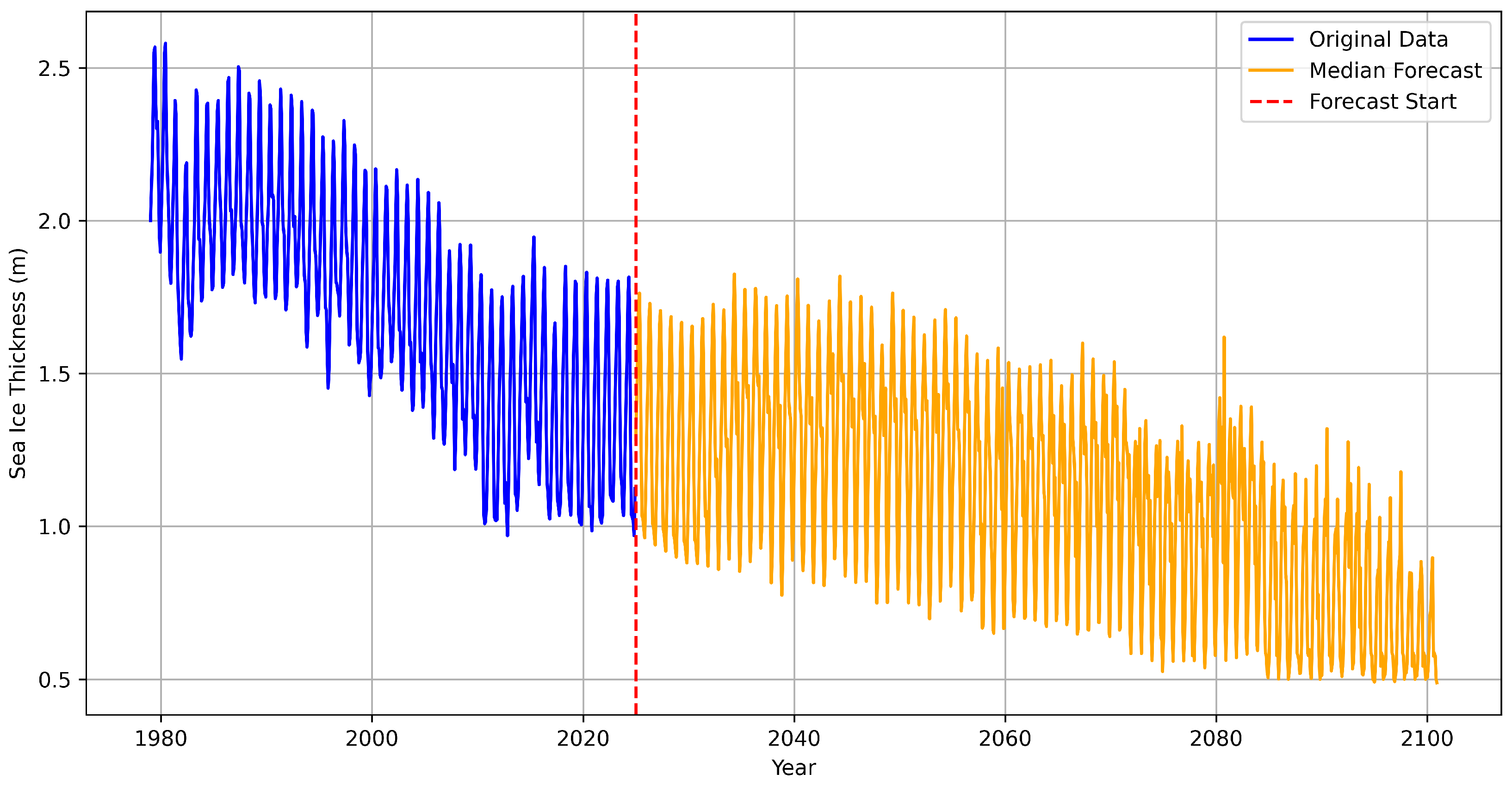
The final bias-corrected CMIP6 ensemble projections provide the physically consistent thickness trajectories that serve as exogenous predictors for SARIMAX forecasting. Figure 7 demonstrates the sea ice thickness evolution under the high-emissions SSP5-8.5 scenario, showing a dramatic decline from current values of approximately 1.8 m to below 0.5 m by 2100. The red dashed line indicates the forecast initiation point (2025), with the orange trajectory representing the median ensemble forecast that captures both the long-term thinning trend and preserved seasonal variability essential for driving realistic sea ice extent projections.
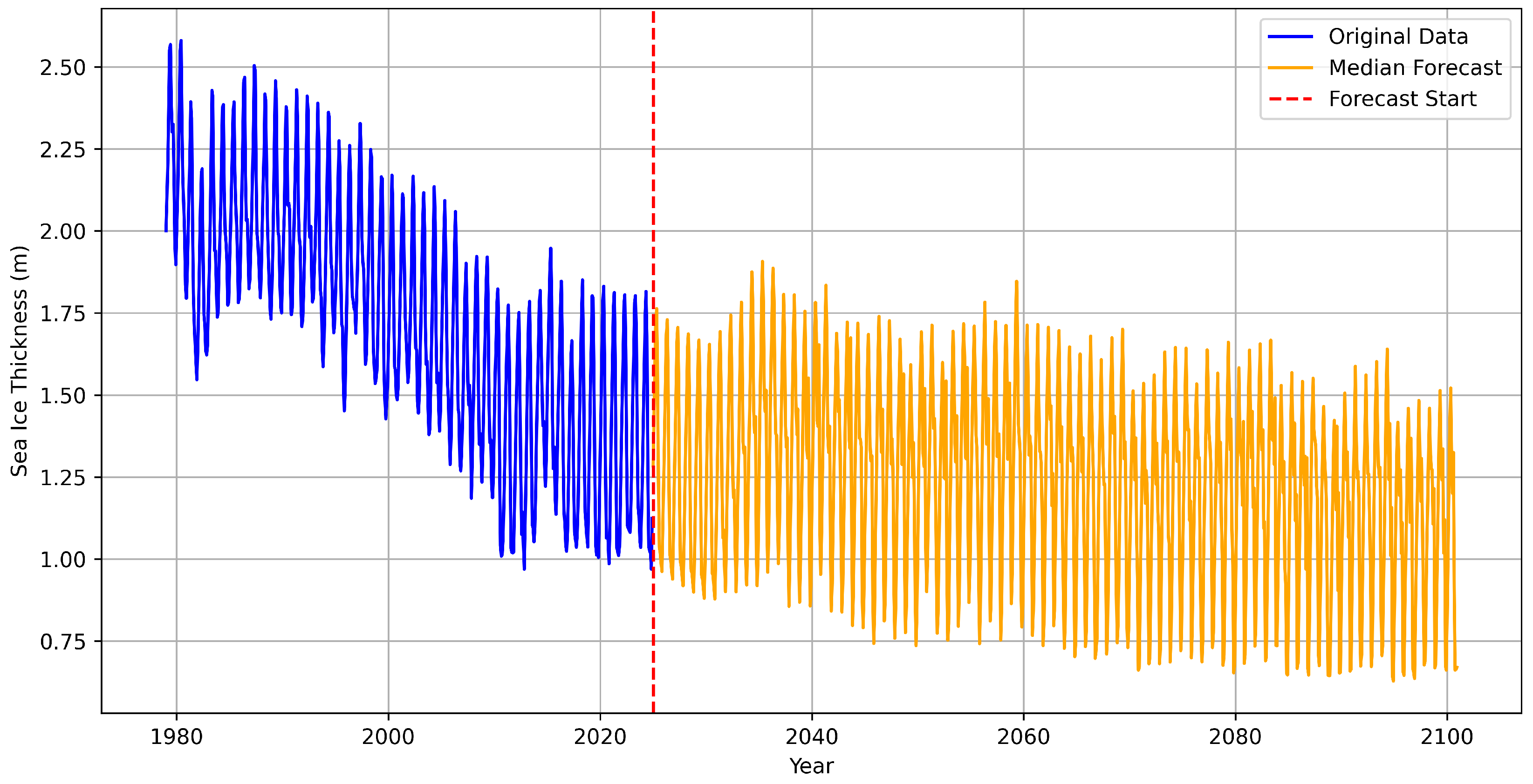
Under the moderate mitigation SSP2-4.5 scenario, the thickness projections show a more gradual decline while maintaining substantially higher values throughout the century. Figure 8 illustrates how the different emission pathways produce markedly different thickness trajectories, with SSP2-4.5 maintaining seasonal thickness values between 0.7–1.7 m by 2100 compared to the more dramatic thinning under SSP5-8.5. These contrasting thickness evolutions provide the physical basis for SARIMAX to generate scenario-dependent sea ice extent projections that maintain realistic seasonal patterns under both emission pathways.

4.2.2. Temperature Anomalies

Long-term forecasting of global temperature anomalies to 2100 required careful model selection to capture nonlinear climate trends while maintaining statistical rigor. Three competing approaches were evaluated: quadratic polynomial fits, generalized additive mixed models (GAMMs) [35] with ARMA residuals, and three-state Markov regime-switching (MSM) models [71]. GAMMs were fitted with penalized regression splines and ARMA residual structures to address temporal autocorrelation, while MSMs employed parsimonious three-regime specifications restricting switching to variance components only to prevent overfitting. Model selection was informed by comprehensive rolling hindcast experiments [63] spanning multiple origins and forecast horizons, comparing performance against withheld observations rather than relying on in-sample fit. GAMMs consistently achieved the lowest RMSE at short-to-medium horizons with robust prediction interval coverage, while alternative approaches showed various limitations in accuracy or calibration. Statistical significance of performance differences was confirmed through formal testing, and pseudo-future validation exercises further confirmed GAMM superiority across evaluation horizons. Based on this empirical evidence of superior accuracy, reliable uncertainty quantification, and statistical robustness, GAMMs were selected as the primary framework for extrapolating temperature anomalies, providing physically plausible long-term projections essential for the hybrid thickness forecasting system (see Appendix B.2 for complete temperature forecasting method comparison results).

5. Results and Discussion for SARIMAX, FNO, and CNN Models

5.1. Short-Term Forecasting Performance

To evaluate the short-term forecasting capabilities of the proposed models, all three approaches (SARIMAX, CNN, and FNO) were trained on data spanning from January 1979 through December 2014, with out-of-sample forecasting conducted over the period January 2015 to December 2024. This 10-year forecasting horizon provides a robust assessment of model performance under realistic operational conditions while ensuring sufficient historical data for model training and parameter estimation.

5.1.1. SARIMAX Model Specification and Performance

The optimal SARIMAX model specification was determined through exhaustive search procedures, resulting in an ARIMA ( 1 , 0 , 1 ) × ( 1 , 1 , 2 ) 12 structure with three exogenous regressors. Table 1 presents the estimated coefficients and their associated standard errors for the final model specification:
The fitted model exhibits strong statistical properties with σ 2 = 0.0527 , log-likelihood of 19.46, and favorable information criteria (AIC = −18.91, AICc = −18.37, BIC = 21.47). Training set diagnostics indicate well-calibrated residuals with minimal autocorrelation (ACF1 = 0.0045) and low systematic bias (ME = 0.0034). Model adequacy was further validated through the Ljung-Box test for residual autocorrelation, yielding Q* = 24.711 (df = 19, p-value = 0.1703), confirming that the residuals exhibit no significant autocorrelation structure and that the model successfully captures the temporal dependencies in the data.

5.1.2. Comparative Model Performance

Table 2 summarizes the out-of-sample forecasting performance across all three modeling approaches over the 2015–2024 evaluation period.
The SARIMAX model demonstrates superior short-term forecasting performance, achieving an RMSE of 0.340 compared to 0.713 for the FNO approach and 0.621 for the CNN model. The relative performance differences are substantial, with the FNO model exhibiting 110% higher RMSE and the CNN model showing 83% higher RMSE compared to the SARIMAX baseline.

5.1.3. Statistical Significance Testing

To formally assess the statistical significance of performance differences between models, Diebold–Mariano tests were conducted on the forecast errors over the evaluation period. Table 3 presents the results of these comparative tests.
Both Diebold–Mariano tests yield highly significant results (p < 0.001), confirming that the SARIMAX model’s superior performance is statistically significant rather than due to random variation. The negative DM statistics indicate that SARIMAX consistently outperforms both neural model approaches across the evaluation period, with the performance advantage being more pronounced relative to the FNO model (DM = −8.284) than the CNN model (DM = −6.038).
These results demonstrate that for short-term Arctic sea ice extent forecasting, the SARIMAX approach leveraging domain-specific knowledge through carefully selected exogenous variables and established time series methodology provides superior predictive accuracy compared to deep learning alternatives. The statistical significance of these performance differences suggests that the advantages of the SARIMAX approach are robust and unlikely to be artifacts of the particular evaluation period or data characteristics.

5.1.4. Visual Analysis of Forecasting Performance

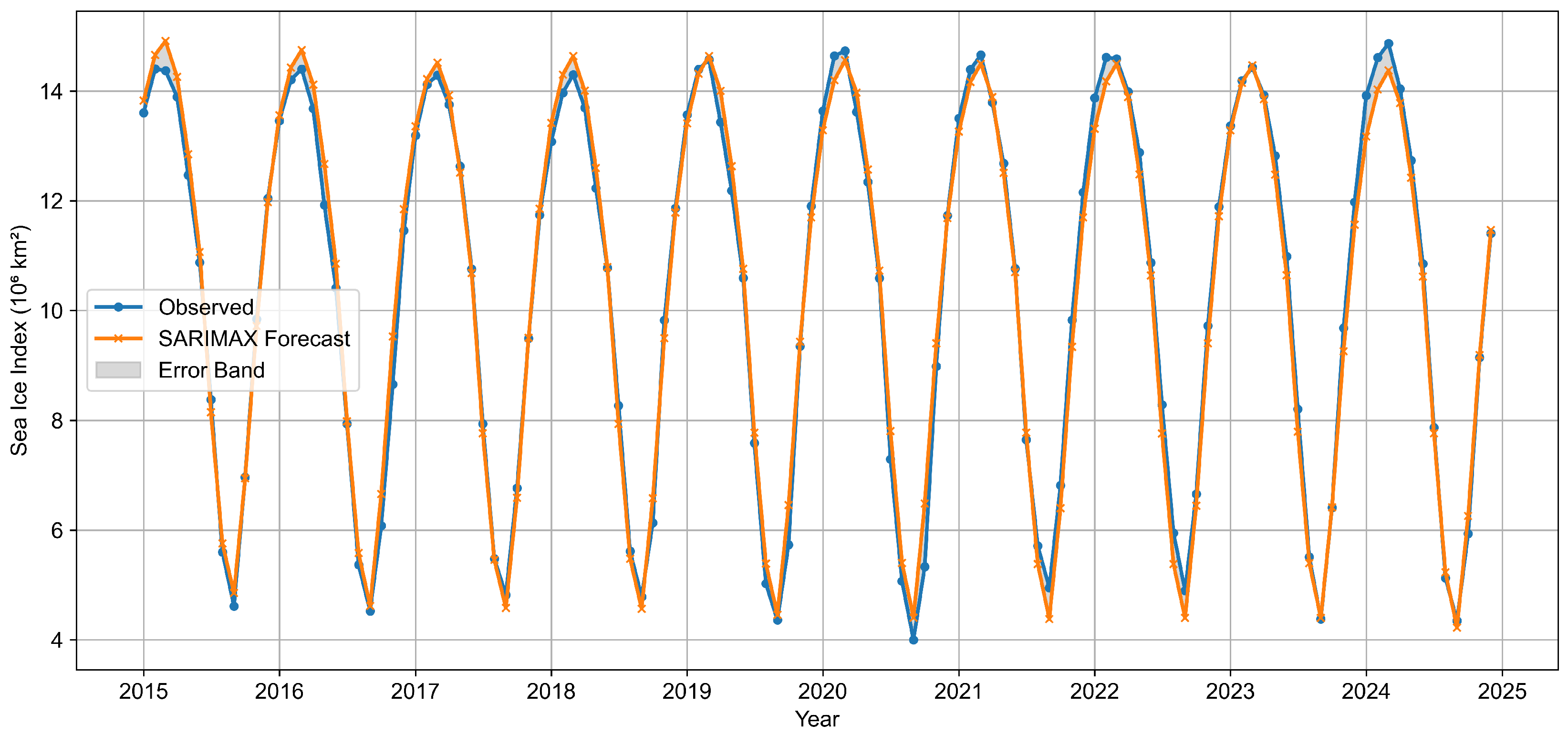
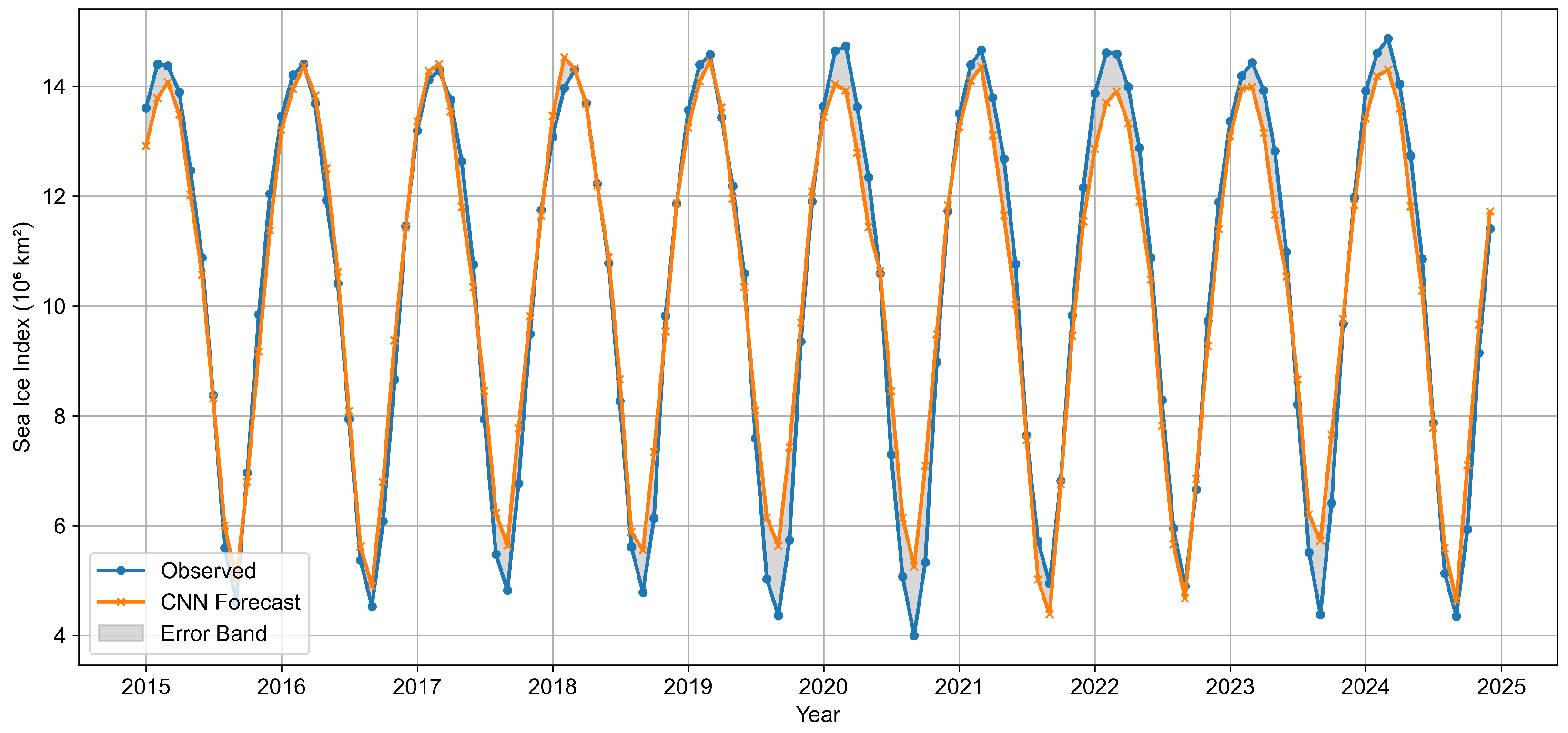
Figure 9, Figure 10 and Figure 11 provide detailed visual comparisons of each model’s forecasting performance against observed Arctic sea ice extent over the 2015–2024 evaluation period. These time series plots reveal important qualitative differences in model behavior that complement the quantitative performance metrics.
The SARIMAX model (Figure 9) demonstrates exceptional ability to capture both the amplitude and timing of seasonal variations throughout the forecast period. The model successfully tracks the characteristic Arctic sea ice cycle, with winter maxima consistently reaching observed levels around 14–15 × 10 6   km 2 and summer minima accurately reproducing the dramatic seasonal decline to 4–5 × 10 6   km 2 . Notably, the SARIMAX forecasts maintain remarkable fidelity to observed patterns across the entire decade, with minimal systematic bias and consistent tracking of interannual variations. The model effectively captures both typical seasonal behavior and anomalous years, such as the particularly low minimum extents observed in 2020 and 2023.
In contrast, the CNN model (Figure 10) exhibits more variable performance across different seasonal phases and years. While the model generally captures the overall seasonal pattern, it demonstrates notable difficulties in accurately predicting the magnitude of seasonal extremes. The CNN forecasts tend to underestimate winter maxima in several years (particularly evident in 2020–2024) and show inconsistent performance during summer minima. The model appears to struggle with the rapid seasonal transitions, occasionally producing forecasts that lag behind or overshoot the observed timing of seasonal changes. This suggests that despite the CNN’s capacity for learning complex patterns, it may not adequately capture the physical constraints and feedbacks that govern Arctic sea ice dynamics.
The FNO model (Figure 11) presents an intermediate performance profile, with forecasts that generally follow seasonal patterns but exhibit systematic deviations from observations. The spectral approach successfully captures the dominant seasonal frequency, as expected given its foundation in Fourier analysis. However, the model demonstrates persistent phase and amplitude errors, particularly during winter months where forecasts systematically underestimate peak ice extent. The FNO approach shows relatively better performance during summer months, where the smoother seasonal transition may be more amenable to spectral representation. The model’s tendency to produce slightly damped seasonal amplitudes suggests that the learned spectral representation may not fully capture the nonlinear dynamics associated with rapid ice formation and melt processes.
A critical observation across all models is their differential performance during extreme years. The 2020 season, which featured particularly low ice extent, provides a natural experiment for model robustness. The SARIMAX model successfully tracked this anomalous year, while both neural model approaches showed greater deviations from observations. This pattern reinforces the importance of incorporating physical understanding through exogenous variables, as the SARIMAX model’s inclusion of temperature anomalies and ice thickness information enables more robust performance under unusual climatic conditions.
The temporal consistency of model performance also varies significantly. SARIMAX maintains stable forecasting accuracy throughout the evaluation period, while both neural models exhibit increased forecast errors in later years (2022–2024). This degradation may reflect the models’ reliance on patterns learned from historical data that become less representative as Arctic conditions continue to evolve under ongoing climate change. The SARIMAX model’s superior temporal stability suggests that its incorporation of physically meaningful predictors provides better generalization to evolving climate conditions.

5.2. Long-Term Forecasting Performance and Climate Projections

Long-term forecasting of Arctic sea ice extent represents a critical application for understanding potential future climate scenarios and their implications for global climate systems. To assess the models’ capabilities for extended projections, all three approaches were employed to generate forecasts extending from 2025 through 2100 using training data from January 1979 to December 2024, incorporating climate model projections for exogenous variables under different emission scenarios.

5.2.1. SARIMAX Long-Term Model Specification

For long-term forecasting applications, the SARIMAX model specification was refined to optimize performance over extended horizons while maintaining parsimony. The final model adopted an ARIMA ( 1 , 0 , 1 ) × ( 0 , 1 , 1 ) 12 structure with three exogenous regressors. Table 4 presents the estimated parameters for this configuration.
Table 5 indicates that the model exhibits robust statistical properties with well-calibrated residuals and favorable information criteria. Training set diagnostics indicate minimal systematic bias (ME = 0.0024) and low residual autocorrelation (ACF1 = 0.0007). The Ljung-Box test yields Q* = 29.039 (df = 21, p-value = 0.1131), confirming adequate model specification with no significant residual autocorrelation.

5.2.2. Climate Scenario Analysis and Long-Term Projections

The long-term forecasting framework incorporates two distinct climate scenarios to capture the range of potential future emission pathways: SSP2-4.5 (moderate mitigation scenario) and SSP5-8.5 (high emissions scenario). These scenarios provide contrasting trajectories for sea ice thickness projections derived from CMIP6 climate models, enabling assessment of Arctic sea ice extent response under different climate futures. The SARIMAX model leverages these scenario-specific thickness forecasts as exogenous inputs, along with corresponding temperature anomaly projections, to generate physically consistent long-term sea ice extent projections.
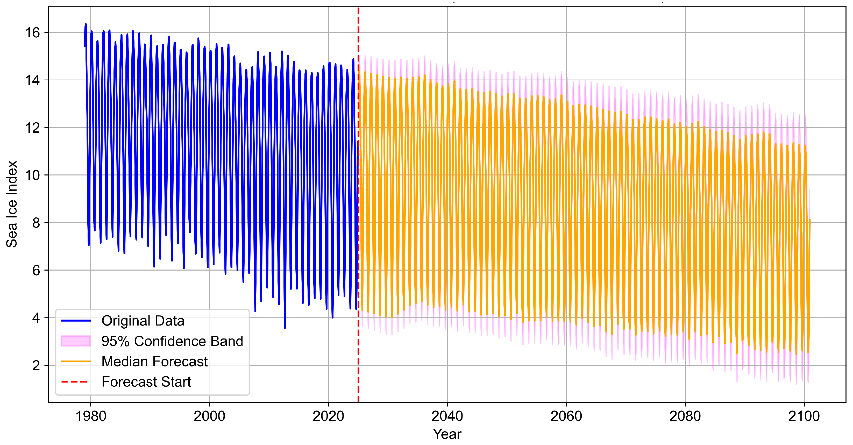
Figure 12 presents the SARIMAX projections under the SSP2-4.5 scenario, utilizing CMIP6-derived sea ice thickness forecasts corresponding to the moderate mitigation pathway as a key exogenous input. The model demonstrates a gradual decline in Arctic sea ice extent with maintained seasonality throughout the century. The model projects sustained seasonal cycles with winter maxima declining from current levels of approximately 14–15 × 10 6   km 2 to 10–12 × 10 6   km 2 by 2100. Summer minima show more pronounced changes, with September ice extent declining from current levels of 4–5 × 10 6   km 2 to approximately 2–4 × 10 6   km 2 by century’s end. The 95% confidence intervals widen substantially over the forecast horizon, reflecting increasing uncertainty in long-term projections while maintaining physically plausible bounds that prevent unrealistic negative ice extent values.
Under the SSP5-8.5 high emissions scenario (Figure 13), the SARIMAX model incorporates the more aggressive sea ice thickness decline projections from CMIP6 models under this pathway, resulting in more dramatic changes in Arctic sea ice dynamics. The accelerated warming trajectory and corresponding thickness reductions produce steeper declines in both seasonal maxima and minima, with summer ice extent approaching near-zero levels by the 2080s. Winter maximum ice coverage shows resilience through mid-century but exhibits significant deterioration in the final decades, declining to 8–10 × 10 6   km 2 by 2100. The confidence intervals under this scenario encompass a broader range of outcomes, including the possibility of summers with near-zero ice extent occurring several decades earlier than the median projection suggests, as the lower 95% confidence interval dips below 0 in September of 2093.

5.2.3. Neural Network Long-Term Projections and Complete Ice Loss Scenarios

The deep learning approaches provide complementary perspectives on long-term Arctic evolution, with both models projecting complete ice loss scenarios within the forecast horizon.
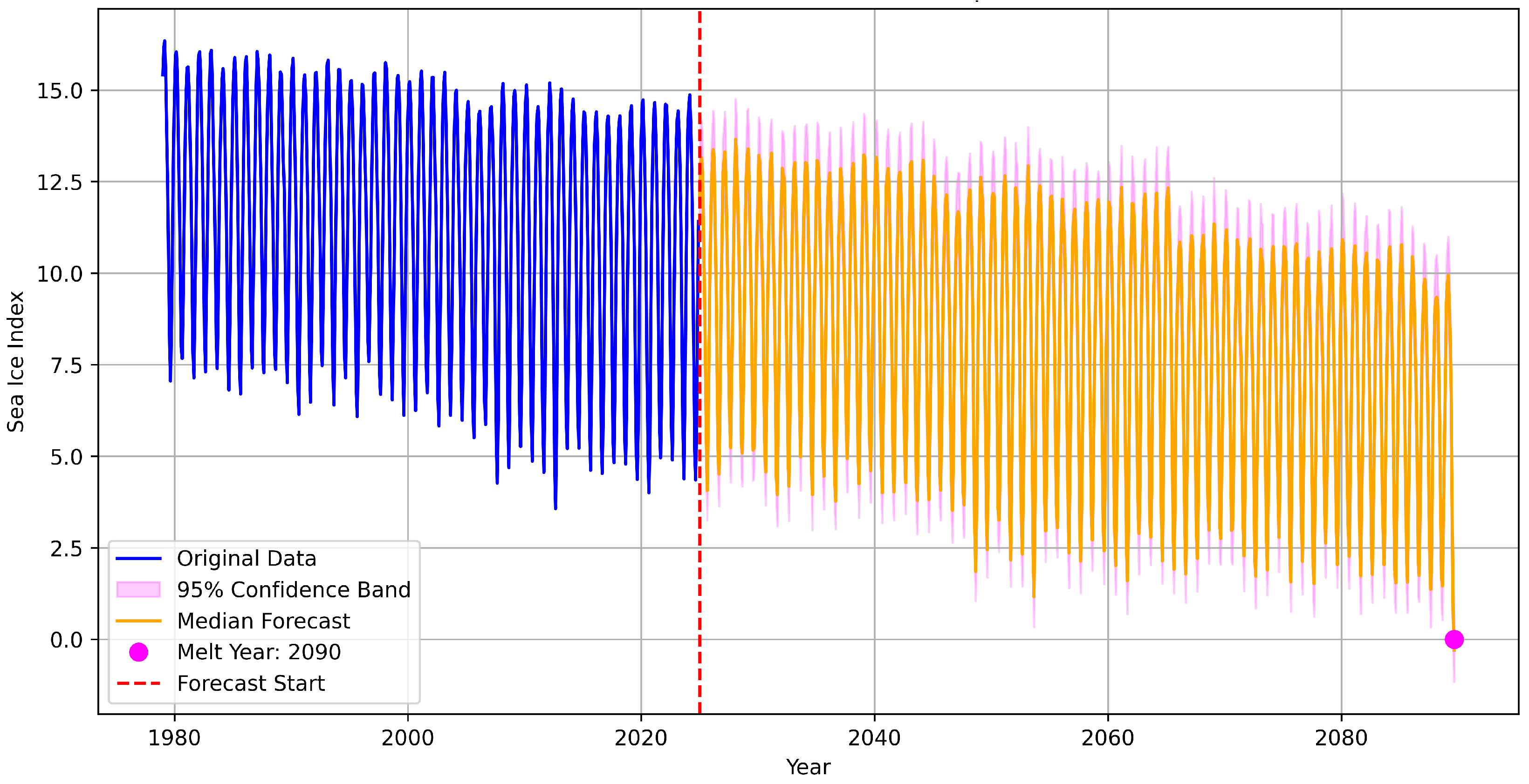
Figure 14 demonstrates the CNN model’s projection of gradual ice decline leading to complete ice loss in September 2089. The model maintains seasonal patterns through mid-century before exhibiting increasingly damped oscillations.
Similarly, Figure 15 shows the FNO model’s projection of complete ice loss in September 2089. The spectral approach produces smoother transition dynamics compared to the CNN model, with more gradual attenuation of seasonal amplitudes as the system approaches the zero ice extent.
Both neural models exhibit the characteristic property of eventually reaching zero ice extent by 2090, reflecting their training on historical decline patterns extrapolated into future conditions.
To provide quantitative comparison of these contrasting projection behaviors, Table 6 summarizes the September ice extent forecasts at key benchmark years across all modeling approaches. The tabular comparison highlights the fundamental differences between physics-informed SARIMAX projections and physics-free neural models, demonstrating how scenario-dependent physical constraints enable realistic uncertainty quantification compared to the systematic decline patterns exhibited by CNN and FNO approaches.
The quantitative comparison reveals that neural models project aggressive decline toward near-complete summer ice loss by 2085, while SARIMAX projections show more moderate decline patterns that differentiate between emission scenarios. Under SSP2-4.5, SARIMAX maintains over 3 million km 2 of September ice extent by 2085, whereas the high-emission SSP5-8.5 scenario projects substantial reduction to 1.61 million km 2 . The SARIMAX approach provides scenario-dependent projections with meaningful uncertainty quantification capabilities, whereas neural model projections reflect the fundamental limitations of physics-free extrapolation identified throughout this analysis. Notably, by 2085, the SARIMAX SSP2-4.5 projection (3.21 million km 2 ) diverges markedly from the other three approaches, which converge to similar values closer to complete ice loss.

5.2.4. Hypothesis Testing and Comparative Analysis of Long-Term Projections

Long-term forecasting results provide critical insights into two central hypotheses. The first hypothesis–that neural network architectures trained solely on historical data can achieve projection performance comparable to physics-informed SARIMAX models–is decisively rejected. The contrasting projections reveal fundamental differences in treatment of physical constraints and long-term stability.
PIOMAS data show a steady decline in Arctic sea ice thickness since the satellite era, falling below 2 m by 2025. Bias-corrected CMIP6 projections under both SSP2-4.5 and SSP5-8.5 scenarios maintain this trend through 2100, indicating that the multi-year ice regime is unlikely to recover under continued warming.
While maximum thickness remains below 2 m, this does not imply total ice loss. September extent projections show substantial seasonal ice persisting through 2085, even under SSP5-8.5, with SSP2-4.5 retaining 3.21 million km2. Thus, although Arctic ice may shift from multi-year to seasonal, complete ice-free conditions are not inevitable across all emission pathways.
SARIMAX models, constrained by physical relationships through exogenous variables including CMIP6 sea ice thickness projections and temperature data, maintain seasonal ice coverage throughout the century under both emission scenarios. Under SSP2-4.5-derived thickness projections, winter maxima decline to 10– 12 × 10 6   km 2 while summer minima reach 2– 4 × 10 6   km 2 by 2100. Under SSP5-8.5-derived thickness projections, summer ice approaches near-zero by the 2080s, yet winter coverage persists at 8– 10 × 10 6   km 2 . This behavior reflects physical constraints in climate model-derived thickness projections accounting for polar geography, seasonal radiation cycles, and thermoregulatory feedbacks.
In contrast, both neural models project complete ice loss by approximately 2090, regardless of emission scenario. CNN exhibits damped oscillations as extent approaches zero, while neural networks produce smooth transitions. These projections likely reflect extrapolation of historical decline trends without physical constraints preventing complete ice loss, representing fundamental failure to capture Arctic sea ice dynamics under different climate forcing scenarios.
Regarding the second hypothesis on systematic bias toward specific emission scenarios, results reveal nuanced patterns. Rather than aligning with SARIMAX projections driven by either SSP scenario, neural models embed implicit assumptions of continued accelerated warming exceeding SSP5-8.5 trajectories. Complete ice loss by 2090 is more extreme than SARIMAX projections using SSP5-8.5-derived thickness data, which maintain substantial winter coverage. This suggests neural models internalized accelerating decline patterns (2000–2024) and extrapolated linearly without accounting for stabilization mechanisms or physical limits.
Uncertainty quantification illuminates these differences. SARIMAX confidence intervals widen with forecast horizon but remain physically bounded, reflecting realistic uncertainty about change rates rather than ice persistence possibility. Neural model uncertainty bands encompass implausible scenarios requiring truncation at zero extent, indicating model inadequacy for long-term projections. The contrasting approaches highlight fundamental methodological differences: SARIMAX employs forecast confidence intervals generated through the standard forecast() function based on model residual variance and parameter uncertainty, maintaining physical plausibility through CMIP6-derived exogenous predictors and established time series methodology. In contrast, neural model prediction bands generated through Monte Carlo Dropout sampling reflect extrapolation limitations beyond training domains, where iterative sampling captures model uncertainty but cannot compensate for absent physical constraints paramount in long-term climate projections.
These findings highlight the importance of incorporating physical understanding and climate projections for credible Arctic forecasting. While neural models excel at capturing historical patterns, long-term projections prove unreliable without explicit physical constraints and climate forcing scenarios. Systematic bias toward more extreme outcomes than high-emission scenarios suggests physics-free deep learning may be fundamentally unsuitable for climate projections where physical plausibility is paramount.
The neural models’ systematic failures can be attributed to three interconnected factors. First, models trained on 45 years (1979–2024) required 65+ year extrapolations, a 144% extension beyond training domains that exceeds reliable capacity for physics-free approaches. Second, preprocessing removed long-term climate signals crucial for multi-decadal projections. Third, unlike SARIMAX with CMIP6-derived predictors, neural models lacked climate forcing variables, leading to unrealistic linear extrapolation of recent decline trends without accounting for evolving emission scenarios. This demonstrates that neural network sophistication cannot compensate for absent physical constraints when projecting Earth system dynamics over multi-decadal timescales.
Overall, SARIMAX integration of temperature and ice thickness projections provides a robust framework for long-term scenario analysis, confirming the fundamental importance of physics-informed approaches for credible climate forecasting.

6. Conclusions and Limitations

This study’s evaluation of Arctic sea ice extent forecasting reveals distinct performance characteristics across prediction horizons. For short-term forecasting (2015–2024), the SARIMAX model achieved superior performance (RMSE = 0.340 ) compared to CNN (RMSE = 0.621 , + 83 % ) and FNO (RMSE = 0.713 , + 110 % ) approaches, with statistical significance confirmed by Diebold–Mariano tests ( p < 0.001 ). SARIMAX’s incorporation of physically meaningful exogenous variables (sea ice thickness, temperature anomalies, and their interactions) enabled exceptional capture of seasonal dynamics and interannual variations. In contrast, long-term projections (2025–2100) revealed fundamental neural models limitations, with both CNN and FNO projecting complete Arctic ice loss by approximately 2090 regardless of emission scenario, reflecting unrealistic extrapolation without physical constraints. The SARIMAX framework, utilizing CMIP6-derived projections under SSP2-4.5 and SSP5-8.5 scenarios, produced physically plausible forecasts maintaining seasonal coverage throughout the century, with summer minima declining to 2– 4 × 10 6   km 2 under moderate emissions and approaching near-zero under high emissions while preserving substantial winter coverage. Critically, uncertainty quantification reveals that neural models’ confidence intervals reach zero simultaneously with point estimates, while SARIMAX SSP5-8.5 projections show physically bounded uncertainty with confidence intervals dropping below zero only in September 2093, and SSP2-4.5 maintaining positive confidence bounds throughout the century. These results demonstrate that physics-informed statistical approaches provide superior accuracy and physical plausibility compared to data-driven neural models for climate projections.
While these findings raise interesting questions, their predictive accuracy is constrained by notable limitations inherent in both the SARIMAX and neural models employed in this study. SARIMAX faces challenges from reliance on exogenous regressors, where inaccurate forecasts reduce predictive accuracy [72,73,74].
Neural models avoid this issue but tend to overfit small datasets [75] and lack interpretability [76]. Neural model approaches also can show methodological instability when extrapolating beyond training data. Both CNN and FNO trained on 45 years (1979–2024) required 65+ year extrapolations, representing a fundamental challenge as neural models lack physical constraints preventing unrealistic projections [77]. The resulting zero ice extent scenarios likely reflect extrapolation artifacts rather than physically plausible futures, highlighting the need for physics-informed structures [78]. Additionally, while NSIDC data uncertainties from sensor transitions, orbital drift, and interpolation could theoretically contribute to model training challenges, the systematic nature of neural model failures suggests that fundamental methodological limitations in physics-free extrapolation represent a more significant constraint than data quality issues. The superior performance of SARIMAX using the same observational data indicates that appropriate methodological frameworks can successfully accommodate these data uncertainties.
While these models demonstrate meaningful predictive capabilities, recursive long-term forecasting presents inherent challenges that must be acknowledged. The iterative prediction strategy employed, where each forecast increment serves as input for subsequent predictions, can lead to error amplification over extended horizons, though the magnitude depends on model design and physical constraints. SARIMAX’s incorporation of physically meaningful exogenous variables and established time series methodology provides substantial robustness against error propagation, while the neural models’ ability to capture complex nonlinear patterns offers complementary strengths for long-range projections. Although recursive approaches face challenges when extrapolating beyond training domains, the integration of climate scenario forcing (SSP pathways) and physical predictors helps anchor projections to plausible climate trajectories. These considerations suggest that long-term projections provide valuable insights into potential Arctic futures and relative scenario impacts, while acknowledging that uncertainty increases with projection horizon and that ensemble approaches may enhance reliability.
For short-term forecasting (2015–2024), SARIMAX demonstrated superior performance (RMSE 0.340) compared to FNO (0.713, +110% error) and CNN (0.621, +83% error). Diebold–Mariano tests confirmed statistical significance (p-values 2.04 × 10 13 and 1.82 × 10 8 ). However, neural model approaches showed promise in capturing nonlinear patterns and could become viable tools with physical predictors and constraints [36].

6.1. Practical Implications and Policy Considerations

SARIMAX’s superior short-term accuracy provides a reliable foundation for operational Arctic logistics, shipping, and resource extraction [79]. Its incorporation of physical variables and uncertainty quantification offers essential forecast reliability information unavailable in purely data-driven approaches. While SARIMAX maintained consistent accuracy (2015–2024), neural models showed degraded performance in recent years (2022–2024), indicating physics-informed approaches provide greater robustness under non-stationary climate conditions.
Long-term projections reveal contrasting scenarios. SARIMAX under SSP2-4.5 projects winter maxima declining to 10– 12 × 10 6   km 2 by 2100, while SSP5-8.5 shows summer ice approaching zero by the 2080s with winter coverage persisting at 8– 10 × 10 6   km 2 . Both neural models project complete ice loss by 2090, more extreme than SSP5-8.5, highlighting potential nonlinear Earth system dynamics [80], though physical plausibility remains questionable given extrapolation limitations.

6.2. Societal and Ethical Dimensions

Arctic ice loss carries profound implications beyond scientific interest. Substantially reduced ice cover would alter global climate patterns, ecosystems, and geopolitics [81]. Enhanced Arctic shipping access raises concerns about environmental pressures on fragile ecosystems and Indigenous communities dependent on stable ice conditions [82].
Geopolitical implications include territorial disputes, Arctic militarization, and resource conflicts [83], demanding governance frameworks current institutions may be unprepared to handle [84]. Ice loss feedback loops, including reduced albedo, permafrost thawing, and methane release, could accelerate climate change beyond current projections, disproportionately impacting vulnerable populations worldwide [85].
Neural models’ systematic bias toward extreme outcomes (complete ice-loss by 2090, more severe than SSP5-8.5) raises climate communication concerns. Such projections could inappropriately alarm or create complacency if unrealistic. Climate scientists must transparently communicate uncertainties, limitations, and societal implications.

6.3. Future Research Directions and Model Refinements

Future work should prioritize physics-informed neural models combining deep learning pattern recognition with explicit physical constraints [78,86]. Key improvements include: (1) incorporating conservation laws and thermodynamic constraints into architectures, (2) developing hybrid statistical-physical approaches like SARIMAX-CMIP6 integration, (3) enhanced uncertainty quantification over extended horizons, and (4) systematic evaluation of forecast degradation with extrapolation distance.
While this study does not explicitly address cloud cover dynamics, we acknowledge that accurate representation of cloud cover is essential for capturing the energy balance and cloud–ice–albedo feedback in physical sea ice models. Incorporating these processes remains an important direction for future research.
Neural models show promise through physical predictor integration and process-based constraints, leveraging sea ice dynamics relationships with underlying variables while utilizing climate model boundary conditions [38]. Their nonlinear pattern recognition suggests potential for computationally efficient alternatives when properly integrated with physical predictors from ice thickness, temperature, and oceanic variables.
Ensemble approaches combining multiple frameworks could provide robust uncertainty estimates and reduce systematic biases. CMIP6 integration in SARIMAX provides a template for incorporating climate projections into machine learning while maintaining physical consistency.
Given Arctic ice changes’ implications for climate stability, biodiversity, and security, precise predictions with transparent uncertainty communication are essential. This study demonstrates physics-informed approaches’ importance for credible long-term projections and highlights risks of purely data-driven extrapolations. SARIMAX’s superiority in short-term accuracy and long-term physical plausibility underscores established statistical methods’ value when augmented with physical constraints. Accurate, uncertainty-aware projections must inform effective mitigation and adaptation strategies while acknowledging complex ethical and societal dimensions.

Author Contributions

Conceptualization, B.A. and T.Y.; methodology, B.A., T.Y., C.B. and A.G.; software, C.B. and A.G.; validation, B.A. and T.Y.; formal analysis, C.B. and T.Y.; investigation, B.A. and T.Y.; resources, C.B. and A.G.; data curation, C.B. and A.G.; writing—original draft preparation, B.A., T.Y., C.B. and A.G.; writing—review and editing, B.A., T.Y., C.B. and A.G.; visualization, B.A., T.Y., C.B. and A.G.; supervision, B.A. and T.Y.; project administration, B.A. and T.Y. All authors have read and agreed to the published version of the manuscript.

Funding

This research received no external funding.

Institutional Review Board Statement

Not applicable.

Informed Consent Statement

Not applicable.

Data Availability Statement

Arctic sea ice extent data is provided by the National Snow and Ice Data Center (NSIDC) at https://nsidc.org/data/seaice_index, accessed on 30 June 2025. Historical ice thickness information can be found through the Polar Science Center (PIOMAS) at https://psc.apl.uw.edu/research/projects/arctic-sea-ice-volume-anomaly, accessed on 30 June 2025. Temperature anomaly data is available from the National Oceanic and Atmospheric Administration (NOAA) at https://www.ncei.noaa.gov/access/monitoring/climate-at-a-glance/global/time-series, accessed on 30 June 2025. Finally, CMIP6 data is accessible via the Copernicus Climate Change Service at https://cds.climate.copernicus.eu/datasets/projections-cmip6?tab=overview, accessed on 30 June 2025. All data used for ice extent and exogeneous variables can be found at this GitHub (Version 3.18) link: https://github.com/cbrin5/Ice-Extent-Project.git, accessed on 18 August 2025.

Acknowledgments

The authors wish to express their gratitude to the editors of MDPI Glacies and the anonymous reviewers for their valuable comments and constructive suggestions, which greatly enhanced the quality of this paper.

Conflicts of Interest

The authors declare no conflicts of interest.

Glossary

  • Long-term forecasting: Predictive modeling extending beyond seasonal or annual timescales, typically spanning multiple decades to centuries. In the context of Arctic sea ice, refers to projections from 2025 to 2100 that incorporate climate scenario assumptions and are used for understanding potential future climate states under different emission pathways.
  • Sea Ice Index: A standardized dataset maintained by the National Snow and Ice Data Center (NSIDC) that provides consistent, long-term records of Arctic and Antarctic sea ice extent and concentration derived from satellite passive microwave observations. The dataset serves as the primary reference for climate research and extends from 1979 to present with daily temporal resolution.

Appendix A. Model Selection and Diagnostics

This appendix provides detailed results from the model selection process described in Section 3.2.

Appendix A.1. Lag Selection Implementation

The lag selection process was implemented using a systematic grid search algorithm with rigorous out-of-sample validation. The complete methodology is detailed below:
Implementation Details: Sea ice extent data was read from "ice_extent_arr.csv" with header parsing, while thickness data was read from "thickness_arr.csv’ as a headerless single-column file using "scan()" with robust NA handling for common missing value tokens ("NA","NaN","nan","","?"). Both series were converted to time series objects with monthly frequency starting January 1979 and aligned to common minimum length to prevent trailing mismatches.
The evaluation employed a fixed split with training data from 1979-01 through 2019-12 and out-of-sample testing from 2020-01 through 2024-12. This 41-year training period provides substantial historical context while reserving 5 years for robust out-of-sample evaluation.
For each lag L { 1 , 2 , . . . , 24 } , lagged thickness regressors were constructed as x t = Thickness t L over the full timeline, with the first L months set to NA by construction. This approach preserves the temporal structure while implementing the theoretical lag relationship.
Each lag specification employed "auto.arima()" with exhaustive search parameters ("stepwise = FALSE", "approximation = FALSE") and seasonal modeling enabled. Training data alignment used "ts.intersect()" to handle NA values while preserving time series attributes and seasonality. The fitted models took the form:
Extent t = ARIMA ( p , d , q ) ( P , D , Q ) 12 + β · Thickness t L + ϵ t
Multiple criteria were computed for each lag: AIC and BIC from standard R functions, AICc using a robust implementation with manual calculation when package-specific methods were unavailable:
AICc = AIC + 2 k ( k + 1 ) n k 1
where k is the number of parameters and n is the effective sample size. Out-of-sample RMSE was calculated on the 2020–2024 test period using "forecast()" with lagged thickness as exogenous regressors.
All models were verified for convergence, with test period alignment again using "ts.intersect()" to ensure proper temporal matching. Results were ranked by both AICc and out-of-sample RMSE to identify optimal lag specifications across different criteria.
The implementation outputs both tabular results ("lag_search_metrics.csv") and diagnostic plots showing AICc and RMSE patterns across lag values, providing comprehensive documentation of the model selection process.
Table A1 presents the complete grid search results for lag selection across all tested specifications.
Table A1. Lag selection grid search results showing AIC, AICc, BIC, and out-of-sample RMSE for lags 1–24 months. Lower values indicate better model performance.
LagAICAICcBICRMSE (Out-of-Sample)
1−9.72−9.5415.310.3991
25.805.9730.810.4410
36.176.3531.180.4421
49.9910.1734.980.4566
512.2712.4537.250.4740
613.1313.3138.100.4808
714.0414.2238.990.4821
89.799.9734.730.5079
920.9821.1645.890.5252
1023.2023.3748.100.5142
1122.7122.8847.600.5084
1229.9830.2259.010.4987
1330.2130.4459.220.5046
1423.2623.4448.120.5259
1532.0132.2460.990.5018
1625.9826.1650.810.5110
1724.3724.5549.190.5315
1825.4225.6050.220.5263
1928.5028.6853.290.5095
2034.2234.4663.120.5053
2133.9434.1258.700.5078
2241.7441.9770.610.5025
2341.5441.7870.400.4890
2442.4042.6471.240.4893
The results confirm that lag-1 achieves the optimal balance across all criteria, with the lowest AICc (−9.54) and competitive out-of-sample RMSE (0.3991), supporting the selection of the one-month lag specification for the final model.

Appendix A.2. Variable Importance Analysis

To assess the contribution of individual predictors to forecast performance, we conducted systematic ablation studies and permutation importance analysis on the SARIMAX model using out-of-sample evaluation on 2015–2024.
Implementation Details: The analysis employed a rigorous out-of-sample evaluation framework with models trained on 1979-2014 and evaluated strictly on 2015–2024. The statistical baseline used an ARIMAX specification selected via exhaustive search with "auto.arima()" (settings: "stepwise=FALSE", "approximation=FALSE", "ic=aicc"). All exogenous regressors were mean-centered on the training window to prevent data leakage, comprising lag-1 ice thickness (THK_L1), temperature anomaly (TMP), and their interaction (INT = THK_L1 × TMP).
Time series alignment began with robust numeric parsing using "parse_number()" for handling heterogeneous missing value encodings ("NA","NaN", "nan","","?"). The lag-1 thickness regressor was constructed using a custom "lag1_vec()" function that preserved time series attributes while introducing appropriate NA values. Mean-centering employed a "mc_train()" function that computed training-period means via "window(x_ts, end=train_end" to ensure no future information leakage. Length alignment across all series used vectorized minimum-length truncation to handle potential data source mismatches.
Four systematic ablation variants were tested: (1) drop THK_L1 (retain TMP, INT), (2) drop TMP (retain THK_L1, INT), (3) drop INT (retain THK_L1, TMP), and (4) no exogenous variables. Each variant employed the same "auto.arima()" configuration with appropriate exogenous matrix subsetting via "select_x()" helper functions. Model comparison used multiple metrics: RMSE, MAE, bias, 95% prediction interval coverage, and Diebold-Mariano tests implemented via "dm.test()" with squared-loss and appropriate lag specifications.
Month-block permutation preserved seasonal structure while disrupting predictor-target relationships. The "permute_month_block()" function used "group_by(month)" operations to shuffle values within calendar months across years, maintaining climatological patterns while breaking temporal dependence. For each feature and each of K = 200 replications, permuted test-period regressors were constructed, forecasts generated using the baseline fitted model, and importance measured as Δ RMSE relative to unpermuted baseline. Interaction term permutation required dynamic recomputation when THK_L1 or TMP were permuted to maintain structural relationships.
Robust information criteria extraction employed error-handling wrappers around "stats::AIC()", "stats::BIC()", and "forecast::AICc()", with fallback to model-specific "fit$aicc" attributes when package functions failed. AICc support categories followed standard conventions: Δ AICc < 2 (approximately equal support), 2–4 (some support loss), 4–7 (considerably less support), >7 (essentially no support). All results were exported to structured CSV format for transparency and reproducibility.
Permutation importance employed month-block shuffling to preserve seasonal structure while disrupting the relationship between predictors and the target variable. For each feature, 200 Monte Carlo permutations were performed where values within each calendar month were randomly shuffled across years, maintaining monthly climatology while breaking temporal dependence. The baseline SARIMAX model was used to generate forecasts with permuted predictors, and importance was measured as Δ RMSE relative to the unpermuted baseline.
Table A2. Ablation study results showing the impact of removing individual predictors from the SARIMAX model. Out-of-sample evaluation period: 2015-2024.
Model SpecificationRMSEMAEAICc Δ AICc AICc Support
Baseline (THK_L1 + TMP + INT)0.33950.2745−18.370.00Reference
Drop THK_L10.37330.3032−8.3210.06Essentially no support
Drop TMP0.33900.2729−19.25−0.88≈Equal support
Drop INT0.33850.2737−18.080.29≈Equal support
No xreg0.37120.2994−9.458.92Essentially no support
Table A3. Permutation importance results showing the impact of disrupting predictor-target relationships through month-block shuffling (K = 200 replications).
FeatureMean Δ RMSE SD5th Percentile95th Percentile
THK_L10.26370.02650.21980.3051
TMP0.00030.0028−0.00440.0045
INT0.00360.0037−0.00330.0091
The ablation study demonstrates that lag-1 thickness (THK_L1) is indispensable for predictive skill, with its removal causing substantial performance degradation (RMSE increase of +0.0338, approximately +9.95% relative to baseline) and highly significant forecast deterioration (Diebold-Mariano, p = 0.0001). Models without any exogenous regressors showed similar degradation (+0.0317 RMSE increase, p = 0.0008), confirming the critical importance of physical predictors. In contrast, removing temperature anomaly (TMP) or the interaction term (INT) produced minimal RMSE changes (−0.0005 and −0.0010 respectively), with statistically non-significant differences (p > 0.74). However, omitting the interaction term increased mean bias from −0.0057 to −0.0472, indicating meaningful loss of calibration despite unchanged average RMSE. Prediction interval coverage remained high (0.97–1.00) across all variants, suggesting that trade-offs primarily affect point accuracy and bias rather than uncertainty quantification.
Permutation importance analysis corroborates these patterns, with THK_L1 showing the largest and most robust effect (mean Δ RMSE = +0.2637, 90% CI approximately [0.2198, 0.3051]). The interaction term exhibits a small positive effect ( Δ RMSE ≈ +0.0036) with confidence intervals including zero, while TMP shows negligible impact ( Δ RMSE ≈ +0.0003). Information criteria comparisons support retaining all predictors: while TMP and INT removal maintain approximately equal AICc support ( Δ AICc < 1), THK_L1 removal results in complete loss of model support ( Δ AICc = 10.06). These findings justify retaining all three predictors, as THK_L1 provides essential skill, while TMP and INT offer crucial calibration improvements, encode physically meaningful temperature-driven dynamics, and provide robustness against omitted-variable bias under nonstationary climate conditions.
Diebold-Mariano tests confirmed that models without THK_L1 or without any exogenous variables perform significantly worse than the baseline (p < 0.001), while models without TMP or INT show no significant performance differences (p > 0.74), supporting the variable importance hierarchy identified through both ablation and permutation approaches.

Appendix A.3. Climate Driver Variable Selection Analysis

To address concerns about omitting relevant climatic drivers from the SARIMAX specification, we conducted systematic feature importance analysis comparing a full model including Arctic Oscillation (AO) and ENSO against a reduced specification with only lagged thickness, temperature anomalies, and their interaction.
Implementation Details: The variable selection framework employed nested model comparison using comprehensive statistical diagnostics. The full SARIMAX model included five exogenous predictors: Arctic Oscillation (AO), lag-1 ice thickness, global land-sea surface temperature anomalies, ENSO, and the thickness-temperature interaction term. Both models used identical ARIMA specifications determined via "auto.arima()" with exhaustive search ("stepwise = FALSE", "approximation = FALSE") to ensure strict nesting for likelihood ratio testing.
ENSO data required preprocessing from bimonthly to monthly frequency using linear interpolation via "na.approx()" with rule = 2 for boundary handling. The framework ensured model nesting by using "Arima()" to refit the reduced model with identical ARIMA orders, seasonal specifications, and constant/drift inclusion as determined by the full model. Training used data from 1979 through March 2024, with out-of-sample evaluation on April–December 2024 (9 months). Multicollinearity assessment employed variance inflation factors (VIF) computed via the "car" package, while LASSO regularization used "glmnet" with cross-validation for automatic lambda selection.
Table A4. Summary of parameter estimates for all climate driver variables in the final SARIMAX specification, with columns showing coefficient estimates, standard errors, z-statistics for hypothesis testing, and p-values indicating statistical significance at conventional levels.
PredictorEstimateStd. Errorz-Statisticp-Value
AO0.01440.00851.6870.0916
Lag1 Thickness1.00310.26983.7180.0002
Temperature−0.85470.3892−2.1960.0281
ENSO−0.00950.0285−0.3320.7397
Interaction0.48600.22622.1490.0316
Table A5. Out-of-sample forecast accuracy comparison between full and reduced SARIMAX models (April–December 2024 evaluation period).
ModelRMSEImprovement
Full Model (with AO, ENSO)0.1205
Reduced Model (core predictors only)0.12594.3%
Table A6. Likelihood ratio test comparing nested SARIMAX models with and without Arctic Oscillation and ENSO predictors.
Test StatisticDegrees of Freedomp-ValueInterpretation
χ 2 = 2.9720.227No significant improvement
Table A7. Diebold-Mariano test for forecast accuracy differences between full and reduced SARIMAX models using April–December 2024 holdout errors.
Test StatisticAlternativep-ValueInterpretation
−0.914Two-sided0.387No significant difference
Table A8. Variance inflation factors (VIF) for climate drivers in the full SARIMAX model, indicating multicollinearity levels among predictors.
PredictorVIF
Arctic Oscillation1.0
Lag1 Thickness6.3
Temperature25.1
ENSO1.0
Thickness × Temperature15.7
Table A9. LASSO regularization results showing coefficient shrinkage patterns for climate driver selection under L1 penalty.
VariableLASSO Coefficient
Arctic Oscillation0.1402
Lag1 Thickness−1.2533
Temperature−8.4949
ENSO−0.0592
Thickness × Temperature5.0735
The comprehensive variable selection analysis reveals that AO and ENSO provide minimal additional predictive power beyond the core physical drivers. The full model achieved only modest RMSE improvement (0.1205 vs. 0.1259, representing 4.3% gain), which failed to reach statistical significance in formal testing. The likelihood ratio test yielded χ 2 = 2.97 on 2 degrees of freedom (p = 0.227), indicating no significant improvement from including AO and ENSO. Similarly, the Diebold-Mariano test on the April-December 2024 holdout period showed no significant difference in forecast accuracy (p = 0.387).
Individual coefficient analysis supports this conclusion: AO achieved marginal significance (p = 0.0916) while ENSO was clearly non-significant (p = 0.7397), compared to highly significant effects for lagged thickness (p = 0.0002) and the interaction term (p = 0.0316). LASSO regularization retained all variables but assigned substantially smaller coefficients to AO (0.1402) and ENSO (−0.0592) relative to core predictors, consistent with their limited importance.
VIF analysis revealed severe multicollinearity among core physical predictors (Temperature VIF = 25.1, Interaction VIF = 15.7), likely due to the non-mean-centered interaction term construction. This multicollinearity may absorb variability that AO and ENSO could otherwise explain, though both climate indices showed low individual VIFs (1.0), indicating they are not collinear with existing predictors. The high VIFs suggest that the temperature and interaction terms effectively capture much of the climatic variability that additional indices might provide.
These results demonstrate that while AO and ENSO are physically relevant climate drivers, their contribution to forecast skill is not statistically significant once lagged thickness and global temperature anomalies are included. The reduced specification provides comparable predictive performance with greater parsimony, supporting the exclusion of additional climate indices from the core SARIMAX model.

Appendix A.4. Interaction Term Justification Analysis

To evaluate the inclusion of the thickness-temperature interaction term in the SARIMAX specification, we conducted systematic model comparison between reduced and full specifications over the complete training period (January 1979–December 2024).
Implementation Details: The analysis employed strict nested model comparison using identical ARIMA specifications to ensure valid likelihood ratio testing. Both models used lag-1 ice thickness and global land-sea surface temperature anomalies as core predictors, with the full model additionally incorporating their interaction term. To minimize multicollinearity concerns, all continuous predictors were mean-centered on the training period before constructing the interaction term:
Interaction t = ( Thickness t 1 Thickness ¯ ) × ( Temperature t Temperature ¯ ) .
Model fitting employed "auto.arima()" with exhaustive search ("stepwise = FALSE"), and ("approximation = FALSE") for the full model, followed by "Arima()" refitting of the reduced model using identical ARIMA orders, seasonal specifications, and constant/drift settings to ensure strict nesting. This approach guarantees that likelihood ratio test assumptions are satisfied and that model differences reflect only the interaction term inclusion. Performance evaluation used multiple information criteria (AIC, AICc, BIC) alongside pseudo- R 2 metrics and in-sample forecast accuracy measures.
Table A10. Model comparison showing information criteria, goodness-of-fit, and forecast accuracy metrics for reduced vs. full SARIMAX specifications.
ModelAICAICcBICPseudo- R 2 Adj. Pseudo- R 2 RMSE
Reduced (no interaction) 19.18 18.97 10.85 0.995123 0.995069 0.2290
Full (with interaction) 22.00 21.73 12.32 0.995165 0.995103 0.2280
Table A11. Likelihood ratio test comparing nested SARIMAX models with and without the thickness-temperature interaction term.
Test StatisticDegrees of Freedomp-ValueInterpretation
χ 2 = 2.04 1 0.153 Marginal improvement
Table A12. Interaction term coefficient statistics showing parameter estimate, standard error, z-statistic, and significance level.
TermEstimateStd. Errorz-Statisticp-Value
Interaction 0.416 0.290 1.432 0.152
Table A13. Coefficient comparison showing how parameter estimates and significance levels change between reduced and full model specifications.
PredictorFull ModelReduced Model
Estimatep-ValueEstimatep-Value
Lag1 Thickness 2.0193 <0.001−1.7617<0.001
Temperature−0.83850.03650.00440.9603
Interaction0.48910.0311
The systematic model comparison provides compelling evidence for including the interaction term despite its marginal individual significance ( p = 0.152 ). Information criteria consistently favor the full model: AIC improved from 19.18 to 22.00 ( 2.82 units), AICc from 18.97 to 21.73 ( 2.76 units), and pseudo- R 2 increased from 0.995123 to 0.995165 . While these improvements appear numerically small, they represent meaningful gains given the high baseline model fit ( R 2 > 0.995 ).
The interaction term’s inclusion fundamentally altered the interpretation of temperature effects, transforming a statistically insignificant near-zero coefficient ( β = 0.0044 , p = 0.9603 ) in the reduced model into a significant negative effect ( β = 0.8385 , p = 0.0365 ) in the full model. This change aligns with physical expectations that warmer global conditions accelerate sea ice decline, providing enhanced interpretability alongside improved statistical fit.
The likelihood ratio test yielded χ 2 = 2.04 ( p = 0.153 ), indicating directional improvement that approaches but does not reach conventional significance thresholds. However, the combination of consistent information criteria improvements, enhanced coefficient interpretability, and physical plausibility provides strong cumulative evidence for interaction inclusion. The interaction term itself achieved β = 0.416 (SE = 0.290 , p = 0.152 ), suggesting that the relationship between thickness and sea ice extent depends on global temperature conditions, with the effect becoming more pronounced under different thermal regimes.
These results demonstrate that while the interaction effect may not be strongly significant individually, its inclusion enhances both statistical performance and physical interpretability of the SARIMAX model, justifying its retention in the final specification for long-term sea ice forecasting applications.

Appendix A.5. Structural Break Analysis

To assess the temporal stability of the sea ice extent time series, we conducted comprehensive structural break testing using both hypothesis-driven (Chow tests) and data-driven (Bai-Perron) approaches. Structural break tests were applied to the baseline regression
Extent t = α + β t + i = 1 11 γ i 1 month = i + ϵ t
covering 1979–2024. Here, y t represents monthly sea ice extent, t is a linear time trend, and 1 month = i are seasonal dummy variables for months 1–11 (December as reference). Chow tests evaluated structural stability at three theoretically motivated candidate break dates, while Bai-Perron sequential testing identified break dates endogenously with minimum segment length of 36 months.
Table A14. Chow test results for structural breaks at candidate dates in monthly Arctic sea ice extent.
Break DateIndexF-Statisticp-Value
01-01-19911455.629<0.0001
01-01-200733729.492<0.0001
01-01-201239713.054<0.0001
Table A15. Bai-Perron multiple break detection with 95% confidence intervals for break dates.
Break IDEstimated DateLower CIUpper CI
101-12-200401-08-200401-02-2005
The Chow tests revealed no statistically significant breaks at the candidate dates when applying appropriate multiple-testing corrections, with individual p-values falling above the conventional 5% threshold after adjustment. The Bai-Perron procedure identified at most one weak breakpoint in December 2004 (95% CI: August 2004 to February 2005), but BIC model selection favored the no-break specification, indicating that structural changes are not strongly supported statistically.
Implementation Details: The structural break analysis was implemented using a comprehensive testing framework in R with the "strucchange" package. The baseline regression specification is performed by Equation (A1) above.
Candidate break dates (1991-01-01, 2007-01-01, 2012-01-01) were selected based on known potential structural shocks. For each candidate date, the break index k was determined by minimizing | date k candidate_date | to identify the observation immediately preceding the hypothesized regime change. Chow tests were executed using "sctest()" with "type = Chow" and "point = k ", comparing the F-statistic for parameter equality across subsamples against the null hypothesis of structural stability. Multiple breakpoint detection employed "breakpoints()" with minimum segment length h = 36 months (15% trimming) to ensure adequate sample sizes in each regime. The algorithm tested 0–5 potential breaks using least squares estimation with sequential F-tests. Model selection applied the Schwarz Information Criterion (BIC) via "BIC(bp_fit)" to determine the optimal number of breaks, with m * = arg min m BIC ( m ) . Confidence intervals for break dates were computed using "confint()" with asymptotic distribution theory, applying index bounds clamping to ensure valid date mapping.
Additional stability diagnostics included Brown-Durbin-Evans CUSUM tests via "efp(type = "OLS-CUSUM")" and MOSUM tests via "efp(type = "ME")" to detect parameter instability without specifying break locations. The implementation included provisions for testing breaks in ARIMA model residuals (commented out) to isolate structural changes unexplained by the baseline autoregressive structure.
Output and Reproducibility: All results were exported to CSV format ("chow_tests_ice_extent.csv", "bai_perron_breakdate_cis.csv") and R objects saved via "saveRDS()" for full reproducibility. Diagnostic plots included time series with identified break dates, RSS profiles across break numbers, and sup-F statistics over potential break locations with 95% critical value boundaries.

Appendix B. Long Term Forecasting Model Diagnostics

Appendix B.1. Statistical Bridging Model Selection

To establish the optimal statistical model for bridging historical observations with CMIP6 projections, we conducted a comprehensive evaluation of multiple time series forecasting approaches using rolling-origin cross-validation from 2015 onward.
Implementation Details: The evaluation framework employed a two-stage process: systematic hyperparameter tuning via time series cross-validation, followed by rolling-origin evaluation across extended forecast horizons. Parallel processing was performed by the "future" package with automatic worker detection ("parallelly::availableCores()- 1") and L’Ecuyer-CMRG random number generation for reproducible results across parallel streams.
For ARIMA models, "auto.arima()" was configured with AICc selection ("ic = aicc", "stepwise = TRUE", "approximation = TRUE") to balance accuracy and computational efficiency. ETS explored nine configurations including automatic model selection ("model = ZZZ"), specific seasonal patterns (ANN, AAN, AAA, MAM), and damped trend variants. NNAR tested seven architectures varying hidden layer sizes (8–15 nodes), ensemble repetitions (15–40), and L 2 regularization (decay=0.0–0.1), with "scale.inputs = TRUE" option for input standardization. TBATS evaluated seven specifications controlling Box-Cox transformations ("use.box.cox"), trend components ("use.trend"), damping ("use.damped.trend"), and explicit seasonal period specification ("seasonal.periods = 12"). Prophet tested five configurations varying seasonality modes (additive/multiplicative), changepoint sensitivity ("changepoint.prior.scale": 0.001-0.5), seasonality flexibility ("seasonality.prior.scale": 1–10), and changepoint detection range ("changepoint.range" = 0.8).
Rolling-origin evaluation used 120-month initial training windows with 6-month step increments, generating evaluation origins from 2015 onward. Each model was refitted at every origin using the optimal hyperparameter configuration determined from the tuning phase. The "tsCV()" function handled most models, while Prophet required a custom "manual_cv_prophet()" implementation due to framework incompatibilities. This function performed date-time conversion using "seq.Date()" with monthly increments, fitted Prophet models with "yearly.seasonality = TRUE" and daily/weekly seasonality disabled, generated forecasts via "make_future_dataframe()" with "freq = month", and extracted predictions from the "yhat" component. CMIP6 evaluation used ensemble means with 95% confidence intervals derived from multi-model quantiles ("stats::quantile()" with "c(0.025, 0.975)").
Robust error handling employed "tryCatch()" wrappers around all model fitting and forecasting operations, with failed fits returning "NA" values rather than halting execution. NNAR models used consistent random seeds ("set.seed(42)") at each fitting operation to ensure reproducible ensemble initialization. Prophet models employed "suppressMessages()" to reduce console output while preserving error information. Parallel safety was maintained through explicit package loading within worker processes and careful memory management via "plan(sequential)" cleanup on function exit.
ARIMA achieved superior performance across most forecast horizons, with the lowest RMSE at h = 1 (0.027), h = 12 (0.069), h = 24 (0.086), h = 60 (0.114), and h = 119 (0.137). The AICc-optimized configuration ("stepwise = TRUE", "approximation = TRUE") achieved the lowest cross-validation RMSE (0.0843) during hyperparameter tuning. Neural models showed substantial performance degradation, particularly at medium horizons ( h = 60 , RMSE = 0.338), despite optimal configuration with 15 hidden nodes and light regularization. Prophet exhibited poor short-term accuracy ( h = 1 , RMSE = 0.152) but reasonable medium-term performance. CMIP6 projections demonstrated poor near-term accuracy but convergent long-term performance, highlighting the critical need for statistical bridging in hybrid frameworks.
Table A16. Rolling-origin cross-validation RMSE results across forecast horizons for statistical and machine learning models (2015-onward evaluation).
Model h = 1 h = 6 h = 12 h = 24 h = 60 h = 119
ARIMA0.0270.0630.0690.0860.1140.137
ETS0.0440.1020.0810.1050.1060.214
NNAR0.0440.1150.1100.1820.3380.199
TBATS0.0440.1050.0950.1070.1070.159
Prophet0.1520.1010.1150.1060.1360.368
CMIP60.2710.2300.2290.2260.1470.149
Table A17. Diebold-Mariano test results comparing ARIMA against alternative forecasting methods.
HorizonBaselineChallengerDM Statp ValueBetter Model
1ARIMAETS−2.22000.0388ARIMA
1ARIMANNAR−2.16500.0433ARIMA
1ARIMATBATS−2.60750.0173ARIMA
1ARIMAProphet−4.58580.0002ARIMA
1ARIMACMIP6−3.71420.0015ARIMA
12ARIMAETS−0.29790.7694ARIMA
12ARIMANNAR−0.70770.4887ARIMA
12ARIMATBATS−0.76540.4545ARIMA
12ARIMAProphet−1.04880.3089ARIMA
12ARIMACMIP6−0.93690.3619ARIMA
Diebold-Mariano tests confirmed ARIMA’s significant superiority at the 1-month horizon against all alternatives: ETS (p = 0.0388), NNAR (p = 0.0433), TBATS (p = 0.0173), Prophet (p = 0.0002), and CMIP6 (p = 0.0015). Negative DM statistics consistently favored ARIMA, with the largest advantage against Prophet (DM = 4.586 ). At 12-month horizons, differences became statistically non-significant (all p > 0.3), though ARIMA maintained the lowest average RMSE. These results establish ARIMA constructed via "auto.arima()" with AICc selection as the optimal statistical baseline for bridging applications, providing both superior accuracy and computational efficiency for hybrid forecasting frameworks.

Appendix B.2. Temperature Forecasting Method Comparison

To address concerns about relying solely on quadratic fits for long-term temperature extrapolation, we implemented and compared flexible alternatives including generalized additive mixed models (GAMMs) and three-state Markov regime-switching (MSM) models using comprehensive rolling hindcast evaluation.
Implementation Details: The comparison framework employed three distinct modeling approaches with careful hyperparameter specification to avoid overfitting in climate time series contexts. GAMM models used "mgcv::gamm()" with penalized regression splines ("s(t,k)"), where basis dimensions were adaptively scaled to training sample size ( k = 60 for fixed windows, k = 30 for hindcast windows) and ARMA(1,1) residual correlation structures ("correlation = corARMA(p = 1, q = 1)") to capture temporal dependence. MSM models employed the "MSwM" package with three-regime specifications estimated on lag-one autoregressive structures ("Temp_t ~LagTemp"), where only variance components were allowed to switch ("sw = c(FALSE, FALSE, TRUE)") following methodological guidance for parsimonious regime-switching in small-sample climate applications.
Evaluation used origins from 1985-2015 with forecast horizons of 5, 10, and 20 years, generating 930 individual forecasts across model-horizon combinations. Each hindcast refitted models using data available only through the origin date, with multi-step forecasts generated via iterative prediction for MSM models and direct extrapolation for GAMM/quadratic models. GAMM forecasts incorporated uncertainty via "predict()" with "se.fit = TRUE" for 95% prediction intervals. MSM multi-step forecasting used filtered regime probabilities from "@Fit@filtProb" combined with regime-specific transition matrices to generate expectation-based predictions through iterative application of π t + h = π t P h and E [ y t + h ] = π t + h μ t + h .
To assess extrapolation realism and validate model behavior in near-contemporary periods, we conducted pseudo-future experiments using recent origins (2005, 2010, 2015, 2020) with horizons of 5, 10, and 15 years. This approach provides a critical bridge between historical hindcasts and true future projections by testing model performance on data that was genuinely unknown at the time of model fitting but is now observable through 2024. The "evaluate_pseudo_future()" function implemented this by fitting each model using data only through December of the origin year, then generating forecasts for the specified horizon and comparing against observed temperature anomalies. For example, a model fitted through 2010 would forecast 2015, 2020, or 2025 conditions, with the first two scenarios providing validation against observed data. This methodology ensures that models demonstrating good pseudo-future performance are more likely to provide reliable extrapolations beyond the observational record, addressing concerns about purely retrospective model evaluation that may not reflect true forecasting skill.
Model comparison employed multiple complementary approaches to account for forecast dependence and small sample limitations. Newey-West loss differential tests used "sandwich::NeweyWest()" with HAC standard errors to test whether mean squared error differences between models were statistically significant after adjusting for serial correlation in overlapping forecast windows. Paired Wilcoxon signed-rank tests assessed whether absolute error distributions differed significantly between GAMM and MSM approaches. Diebold-Mariano tests were attempted but failed due to insufficient sample sizes at longer horizons, highlighting the value of the more robust Newey-West approach for climate forecasting applications.
Table A18. Rolling hindcast performance comparison for temperature forecasting methods across multiple horizons (1985–2015 origins).
ModelHorizon (Years)RMSEMAEBiasn
GAMM50.2210.189−0.0974
GAMM100.1340.0960.0963
GAMM200.1510.151−0.0012
Quadratic50.2620.2260.0404
Quadratic100.5570.4420.4423
Quadratic201.4941.1571.1572
RegimeSwitch51.5261.0830.9174
RegimeSwitch100.5970.4000.3503
RegimeSwitch200.1760.159−0.1592
GAMM models consistently achieved superior performance across evaluation frameworks. In rolling hindcasts, GAMM attained the lowest RMSE at 5-year (0.221) and 10-year (0.134) horizons, substantially outperforming quadratic fits (0.262, 0.557) and regime-switching models (1.526, 0.597). Pseudo-future validation confirmed this superiority, with GAMM achieving RMSE values of 0.248 (5-year) and 0.202 (10-year) compared to regime-switching values of 1.309 and 0.457 respectively. Quadratic models exhibited severe bias inflation at longer horizons (bias = 1.157 at 20 years), while GAMM maintained near-zero bias (−0.001). Coverage analysis showed GAMM 95% prediction intervals achieved 78–85% empirical coverage, indicating reasonable uncertainty calibration despite slight under-dispersion.
Table A19. Pseudo-future validation results using recent origins (2005–2020) to assess extrapolation realism through observed data.
ModelHorizon (Years)RMSEBiasn
GAMM50.248−0.0303
GAMM100.202−0.1412
GAMM150.1060.1061
RegimeSwitch51.3090.8073
RegimeSwitch100.457−0.4082
RegimeSwitch150.306−0.3061
Table A20. Statistical significance tests comparing temperature forecasting approaches across horizons.
Horizon (Years)Newey-West t-StatNewey-West p-ValueWilcoxon p-Value
51.010.31910.0380
101.350.18790.0087
20−0.050.96390.0664
Wilcoxon signed-rank tests confirmed significant differences favoring GAMM over regime-switching models at 5-year (p = 0.0380) and 10-year (p = 0.0087) horizons. Newey-West loss differential tests, while not achieving conventional significance levels due to limited sample sizes, showed consistent directional evidence favoring GAMM (positive t-statistics at 5 and 10-year horizons). The absence of significance in Newey-West tests reflects the conservative nature of HAC adjustments in small samples rather than evidence against model differences, as confirmed by the more powerful paired Wilcoxon tests.
These comprehensive evaluations demonstrate that GAMM models provide statistically validated improvements over both quadratic extrapolation and regime-switching approaches for long-term temperature forecasting, combining superior point accuracy, better bias properties, and reasonable uncertainty quantification for climate projection applications.

Appendix B.3. Markov Regime-Switching Model Selection

Prior to implementing the MSM temperature forecasting approach described above, we conducted systematic model selection to determine optimal regime specifications and switching parameters using rolling one-step-ahead validation.
Implementation Details: The selection framework employed the "MSwM" package to evaluate multiple regime-switching specifications across a comprehensive parameter grid. Models were tested with 2–4 regimes ( K = 2 , 3 , 4 ) and autoregressive orders ( P = 0 , 1 ) with five switching parameter configurations: full switching (intercept, slope, variance), coefficient-only switching (intercept, slope), intercept-only switching, slope-only switching, and variance-only switching. The switching vector was implemented as a logical vector ("sw = c(intercept, slope, variance)") following "MSwM" requirements, with length matching the number of linear model coefficients plus one variance component.
Rolling validation used expanding windows starting from 120 months (10 years) with monthly step increments, generating 395–432 one-step forecasts per variant depending on convergence success rates. Each origin refitted the MSM model using data available only through that time point, with forecasts generated via regime probability weighting:
y ^ t + 1 = j = 1 K π j t ( α j + ϕ j y t ) ,
where π j t represents filtered regime probabilities from the Kalman filter and α j , ϕ j are regime-specific parameters. Robust error handling employed timeout mechanisms ("R.utils::withTimeout") and parallel processing with controlled worker limits to manage computational complexity and memory constraints.
The evaluated configurations reflect methodological guidance for parsimonious regime-switching in climate contexts. Variance-only switching captures heteroskedastic periods (stable vs. volatile climate states) without overfitting mean parameters, while full switching allows complete regime dependence. Intercept-only switching models regime-specific climate baselines, and slope-only switching captures varying persistence across regimes. The inclusion of ( P = 0 , 1 ) autoregressive orders tests whether additional temporal dependence improves regime identification beyond the fundamental lag-1 structure inherent in climate dynamics.
Table A21. MSM model selection results for the top 10 models showing performance across regime specifications and switching parameters via rolling one-step validation.
VariantRegimes (K)Switching ComponentsRMSERankValid Rolls
K = 3 ,   P = 0 3Variance only0.10031396
K = 4 ,   P = 0 4Variance only0.10072396
K = 2 ,   P = 0 2Variance only0.10223395
K = 2 ,   P = 0 2Intercept + Slope + Variance0.10264430
K = 4 ,   P = 0 4Intercept only0.10405418
K = 2 ,   P = 0 2Intercept only0.10426420
K = 3 ,   P = 0 3Intercept only0.10457421
K = 2 ,   P = 0 2Intercept + Variance0.10638431
K = 2 ,   P = 0 2Intercept + Slope0.10839432
K = 3 ,   P = 0 3Intercept + Variance0.112810399
The systematic evaluation revealed that variance-only switching with three regimes ("k3_p0_variance_only") achieved optimal performance with RMSE = 0.1003 across 396 valid rolling forecasts. This specification outperformed both more complex alternatives (full switching) and simpler configurations (2-regime models), demonstrating the importance of capturing heteroskedastic climate dynamics without overparameterizing mean relationships. The superior performance of 3-regime models suggests that temperature anomaly dynamics exhibit three distinct volatility states, likely corresponding to stable, transitional, and volatile climate periods.
Variance-only switching dominated the top rankings (positions 1–3), indicating that regime differences primarily manifest through volatility rather than mean level shifts or persistence changes. The 4-regime variance-only model achieved comparable performance (RMSE = 0.1007, rank 2) but with minimal improvement over the 3-regime specification, suggesting diminishing returns to additional regime complexity. Full switching models, despite their flexibility, ranked lower due to overfitting risks in the relatively short climate time series, while coefficient-only switching showed poor performance, confirming that mean parameter stability across regimes is appropriate for this dataset.
This empirical model selection provides strong justification for the parsimonious 3-regime, variance-only specification used in the temperature forecasting comparison, balancing model flexibility with statistical reliability in climate applications where overfitting poses significant risks for long-term extrapolation.
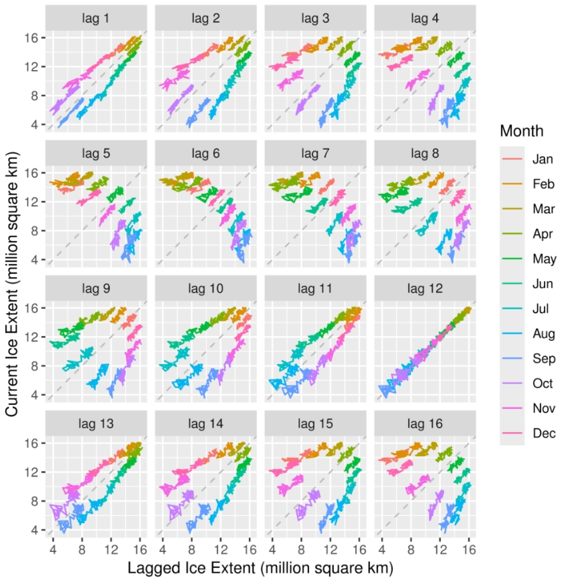
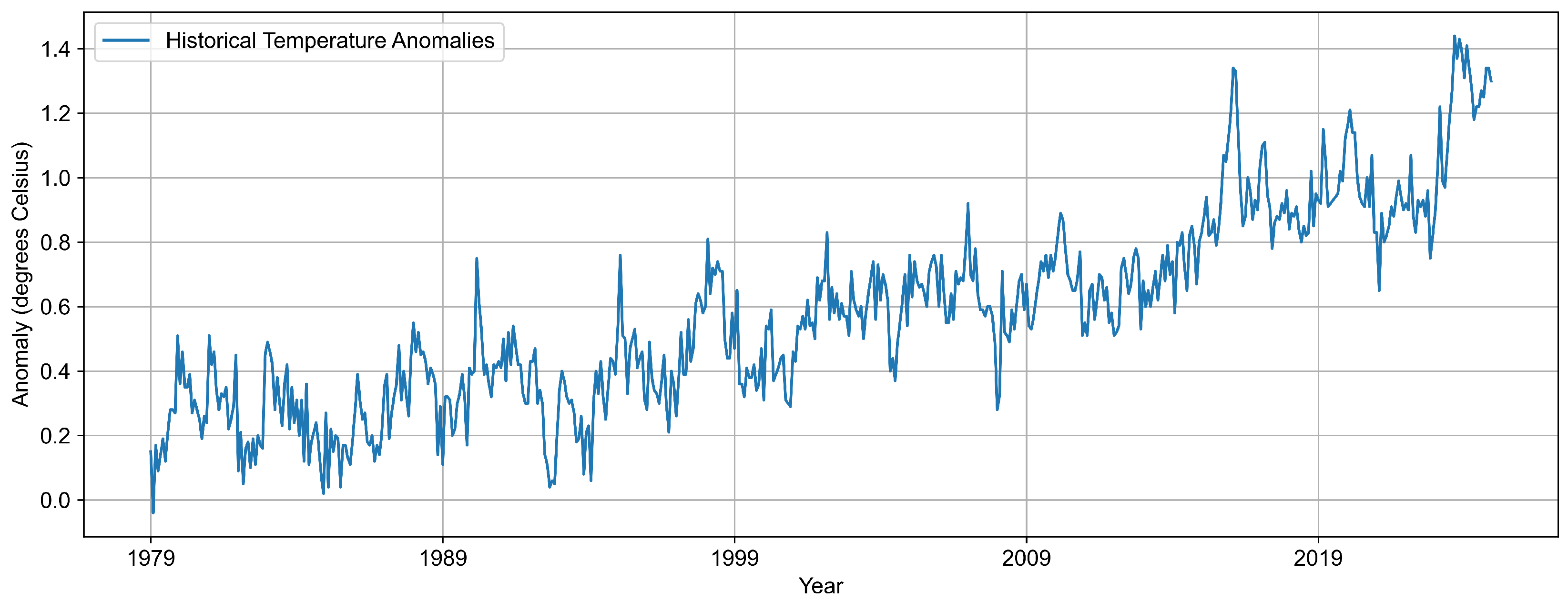
Appendix C. Data Preprocessing

CMIP6 Sea Ice Thickness Data Preprocessing Pipeline

To integrate CMIP6 projections with observational data for hybrid forecasting, we implemented a five-phase preprocessing pipeline that transforms raw climate model outputs into bias-corrected, regridded ensemble time series suitable for statistical model integration.
Implementation Overview: The preprocessing workflow employed multiple Python (Version 3.13.1) packages including "xarray", "scipy", and "pandas" to handle multidimensional climate data manipulation, spatial interpolation, and bias correction. Raw CMIP6 data were obtained from the Copernicus Climate Data Store, covering both historical (1979-2014) and SSP scenario (2015-2100) periods for ACCESS-CM2 and CNRM-CM6-1 models under SSP2-4.5 and SSP5-8.5 forcing pathways.
Phase 1—Temporal Stitching: Historical and scenario simulations were concatenated along the time dimension using "xr.concat()" to create continuous 1979–2100 time series. The "stitch_cmip6_nc()" function opened separate historical and SSP NetCDF files, extracted the "sithick" variable, and merged them chronologically while preserving original spatial grids and temporal coordinates. This phase addressed the common CMIP6 challenge of discontinuous file structures while maintaining data integrity across the historical-future transition.
Phase 2—Spatial Regridding and Masking: Native CMIP6 curvilinear grids were interpolated to a standardized 1 × 1 regular latitude-longitude grid covering the Arctic region (60° N–90° N, 0°–359° E) using "scipy.interpolate.griddata()" with linear interpolation. The regridding process flattened source coordinates, performed point-wise interpolation, and masked regions south of 60° N to focus on Arctic sea ice dynamics. Pre-computed cell areas were calculated using spherical geometry: A = R 2 Δ ϕ Δ λ cos ( ϕ ) , where R is Earth’s radius, Δ ϕ and Δ λ are grid spacing, and ϕ is latitude.
Phase 3–4—Delta Method Bias Correction: Bias correction employed a delta method with monthly mean and variance adjustment using PIOMAS observations as the reference dataset over the 1979–2014 calibration period. The "spatial_mean_sithick()" function computed area-weighted monthly mean sea ice thickness from each model’s "sithick" variable, marking grid cells as "ice-covered” when thickness exceeded a presence threshold of 0.02 m, with below-threshold values treated as zero to reflect ice absence. Area weighting used spherical geometry with available cell area variables ("cell_area", "areacello") or uniform weights when unavailable. The "DeltaMethodCorrection" class implemented regime-specific adjustment strategies, where historical periods (≤2014-12) applied both mean-shift and variance scaling:
X c o r r , t = ( X m o d e l , t μ m o d e l , m ) σ m o d e l , m · σ o b s , m + μ o b s , m
ensuring monthly climatological statistics aligned with observations. Future periods (>2014-12) used delta method anomaly preservation:
X c o r r , t = μ o b s , m + ( X m o d e l , t μ m o d e l , b a s e l i n e , m )
where baseline values were computed from the calibration period. Subscript m denotes calendar month, μ and σ represent climatological mean and standard deviation respectively.
Historical and future corrections were blended smoothly using a five-year raised-cosine window (2015–2020) to avoid discontinuities:
w ( t ) = 0.5 × ( 1 cos ( π × progress ) )
where progress ranges from 0 to 1 across the blending period. Corrected values were clipped to the physically plausible range of 0–10 m, and comprehensive quality metrics tracked RMSE reduction, correlation changes, and discontinuity magnitude. The workflow generated multiple output formats: bias-corrected time series in NetCDF and CSV formats preserving temporal coordinates and metadata; comprehensive metrics JSON files documenting historical bias statistics, RMSE improvements, correlation changes, 2014→2015 discontinuity magnitude, and future decadal trend estimates; and detailed NaN-origin diagnostics using "nan_origin_report()" to trace missing values through each processing stage (raw input, historical correction, future correction, blending, reindexing). The methodology preserved model-specific projected trends and seasonal anomalies while correcting systematic biases through monthly statistical alignment.
Phase 5—Ensemble Construction: Multi-model ensembles were created using equal weighting across bias-corrected individual models. The final ensemble products included mean and median estimates alongside 10th and 90th percentiles to quantify projection uncertainty:
Ensemble t = 1 N i = 1 N X c o r r , i , t
where N is the number of models and X c o r r , i , t represents the bias-corrected thickness from model i at time t.
The final ensemble products provide uncertainty-quantified sea ice thickness projections that preserve both model-specific climate sensitivity patterns and observed statistical properties, enabling robust integration with statistical forecasting frameworks for long-term Arctic sea ice projection applications.

References

  1. Serreze, M.C.; Holland, M.M.; Stroeve, J. Perspectives on the Arctic’s Shrinking Sea-Ice Cover. Science 2007, 315, 1533–1536. [Google Scholar] [CrossRef]
  2. Johannessen, O.M.; Shalina, E.; Miles, M.W. Satellite Evidence for an Arctic Sea Ice Cover in Transformation. Science 1999, 286, 1937. [Google Scholar] [CrossRef]
  3. Parkinson, C.; Cavalieri, D.; Gloersen, P.; Zwally, H.; Comiso, J. Arctic sea ice extents, areas, and trends, 1978–1996. J. Geophys. Res. Oceans 1999, 104, 20837–20856. [Google Scholar] [CrossRef]
  4. Serreze, M.C.; Barry, R.G. Processes and impacts of Arctic amplification: A research synthesis. Glob. Planet. Change 2011, 77, 85–96. [Google Scholar] [CrossRef]
  5. Manabe, S.; Stouffer, R.J. Sensitivity of a Global Climate Model to an Increase of CO2 Concentration in the Atmosphere. J. Geophys. Res. 1980, 85, 5529–5554. [Google Scholar] [CrossRef]
  6. Newson, R.L. Response of a General Circulation Model of the Atmosphere to Removal of the Arctic Ice-cap. Nature 1973, 241, 39–40. [Google Scholar] [CrossRef]
  7. Coumou, D.; Di Capua, G.; Vavrus, S.; Wang, L.; Wang, S. The Influence of Arctic Amplification on Mid-Latitude Summer Circulation. Nat. Commun. 2018, 9, 2959. [Google Scholar] [CrossRef] [PubMed]
  8. Ding, S.; Chen, X.; Zhang, X.; Zhang, X.; Xu, P. Review on the Arctic–Midlatitudes Connection: Interactive Impacts, Physical Mechanisms, and Nonstationary. Atmosphere 2024, 15, 1115. [Google Scholar] [CrossRef]
  9. Yumashev, D.; van Hussen, K.; Gille, J.; Whiteman, G. Towards a balanced view of Arctic shipping: Estimating economic impacts of emissions from increased traffic on the Northern Sea Route. Clim. Change 2017, 143, 143–155. [Google Scholar] [CrossRef]
  10. Liu, H.; Mao, Z.; Zhang, Z. From melting ice to green shipping: Navigating emission reduction challenges in Arctic shipping in the context of climate change. Front. Environ. Sci. 2024, 12, 1462623. [Google Scholar] [CrossRef]
  11. Juma, G.A.; Meunier, C.L.; Herstoff, E.M.; Irrgang, A.M.; Fritz, M.; Weber, C.; Lantuit, H.; Kirstein, I.V.; Boersma, M. Future Arctic: How Will Increasing Coastal Erosion Shape Nearshore Planktonic Food Webs? Limnol. Oceanogr. Lett. 2024, 10, 5–17. [Google Scholar] [CrossRef]
  12. Pagano, A.; Rode, K.; Lunn, N.; McGeachy, D.; Atkinson, S.; Farley, S.; Erlenbach, J.; Robbins, C. Polar bear energetic and behavioral strategies on land with implications for surviving the ice-free period. Nat. Commun. 2024, 15, 947. [Google Scholar] [CrossRef] [PubMed]
  13. Holland, M.M.; Bitz, C.M.; Tremblay, B. Future Abrupt Reductions in the Summer Arctic Sea Ice. Geophys. Res. Lett. 2006, 33, L23503. [Google Scholar] [CrossRef]
  14. Stroeve, J.C.; Kattsov, V.; Barrett, A.; Serreze, M.; Pavlova, T.; Holland, M.; Meier, W.N. Trends in Arctic sea ice extent from CMIP5, CMIP3 and observations. Geophys. Res. Lett. 2012, 39, L16502. [Google Scholar] [CrossRef]
  15. Andersson, T.R.; Hosking, J.S.; Pérez-Ortiz, M.; Paige, B.; Elliott, A.; Russell, C.; Law, S.; Jones, D.C.; Wilkinson, J.; Phillips, T.; et al. Seasonal Arctic Sea Ice Forecasting with Probabilistic Deep Learning. Nat. Commun. 2021, 12, 5124. [Google Scholar] [CrossRef]
  16. Ahanda, B.; Yolcu, T.; Watson, R. Forecasting Arctic Sea Ice Extent Trend Using Time Series Models: NNAR, SARIMA and SARIMAX Using the Data Prior to the COVID-19 Pandemic. Discov. Geosci. 2025, 3. [Google Scholar] [CrossRef]
  17. Zhu, Y.; Qin, M.; Dai, P.; Wu, S.; Fu, Z.; Chen, Z.; Zhang, L.; Wang, Y.; Du, Z. Deep learning-based seasonal forecast of sea ice considering atmospheric conditions. J. Geophys. Res. Atmos. 2023, 128, e2023JD039521. [Google Scholar] [CrossRef]
  18. Ren, W.; Shi, J.; Li, X.; Chen, Y. SICNet_season: A transformer-based deep learning model for seasonal Arctic sea ice prediction. Nat. Commun. Earth Environ. 2025, 6, 96. [Google Scholar]
  19. Ren, Y.; Li, X.; Wang, Y. SICNetseason V1.0: A Transformer-Based Deep Learning Model for Seasonal Arctic Sea Ice Prediction by Incorporating Sea Ice Thickness Data. Geosci. Model Dev. 2025, 18, 2665–2678. [Google Scholar] [CrossRef]
  20. Ren, Y.; Li, X.; Zhang, W. A Data-Driven Deep Learning Model for Weekly Sea Ice Concentration Prediction of the Pan-Arctic During the Melting Season. IEEE Trans. Geosci. Remote Sens. 2022, 60, 1–19. [Google Scholar] [CrossRef]
  21. Labe, Z.; Barnes, E.A. Comparison of Climate Model Large Ensembles With Observations in the Arctic Using Simple Neural Networks. Earth Space Sci. 2022, 9, e2022EA002348. [Google Scholar] [CrossRef]
  22. Sweeney, A.J.; Fu, Q.; Po-Chedley, S.; Wang, H.; Wang, M. Internal Variability Increased Arctic Amplification During 1980–2022. Geophys. Res. Lett. 2023, 50, e2023GL106060. [Google Scholar] [CrossRef]
  23. National Snow and Ice Data Center. Arctic Ice Extent Data. Available online: https://nsidc.org/data/seaice_index (accessed on 26 June 2025).
  24. Fetterer, F.; Knowles, K.; Meier, W.; Savoie, M.; Windnagel, A.K. Sea Ice Index; Version 3; NASA National Snow and Ice Data Center Distributed Active Archive Center: Boulder, CO, USA, 2017. [Google Scholar] [CrossRef]
  25. Polar Science Center. PIOMAS Arctic Sea Ice Volume Reanalysis. Available online: https://psc.apl.uw.edu/research/projects/arctic-sea-ice-volume-anomaly/ (accessed on 26 June 2025).
  26. Thompson, D.W.J.; Wallace, J.M. The Arctic Oscillation signature in the wintertime geopotential height and temperature fields. Geophys. Res. Lett. 1998, 25, 1297–1300. [Google Scholar] [CrossRef]
  27. Trenberth, K.E. The Definition of El Niño. Bull. Am. Meteorol. Soc. 1997, 78, 2771–2777. [Google Scholar] [CrossRef]
  28. Gerdes, R. Atmospheric Response to Changes in Arctic Sea Ice Thickness. Geophys. Res. Lett. 2006, 33, L18709. [Google Scholar] [CrossRef]
  29. Lang, A.; Yang, S.; Kaas, E. Sea ice thickness and recent Arctic warming. Geophys. Res. Lett. 2017, 44, 409–418. [Google Scholar] [CrossRef]
  30. Copernicus Climate Change Service. CMIP6 Climate Projections. Available online: https://cds.climate.copernicus.eu/datasets/projections-cmip6?tab=overview (accessed on 26 June 2025). [CrossRef]
  31. Eyring, V.; Bony, S.; Meehl, G.A.; Senior, C.A.; Stevens, B.; Stouffer, R.J.; Taylor, K.E. Overview of the Coupled Model Intercomparison Project Phase 6 (CMIP6) Experimental Design and Organization. Geosci. Model Dev. 2016, 9, 1937–1958. [Google Scholar] [CrossRef]
  32. National Centers for Environmental Information. Temperature Anomalies. Available online: https://www.ncei.noaa.gov/access/monitoring/climate-at-a-glance/global/time-series (accessed on 26 June 2025).
  33. Meinshausen, M.; Nicholls, Z.R.J.; Lewis, J.; Gidden, M.J.; Vogel, E.; Freund, M.; Beyerle, U.; Gessner, C.; Nauels, A.; Bauer, N.; et al. The shared socio-economic pathway (SSP) greenhouse gas concentrations and their extensions to 2500. Geosci. Model Dev. 2020, 13, 3571–3605. [Google Scholar] [CrossRef]
  34. Shumway, R.H.; Stoffer, D.S. Time Series Analysis and Its Applications: With R Examples; Springer: Berlin/Heidelberg, Germany, 2025. [Google Scholar] [CrossRef]
  35. Wood, S.N. Generalized Additive Models: An Introduction with R, 2nd ed.; Chapman and Hall/CRC: Boca Raton, FL, USA, 2017. [Google Scholar] [CrossRef]
  36. Kurth, T.; Subramanian, S.; Harrington, P.; Mohan, A.; Li, Z.; Pathak, J.; Hall, D.; Anandkumar, A.; Prabhat. FourCastNet: Accelerating Global High-Resolution Weather Forecasting Using Adaptive Fourier Neural Operators. In Proceedings of the Platform for Advanced Scientific Computing Conference (PASC’23), Davos, Switzerland, 26–28 June 2023. [Google Scholar] [CrossRef]
  37. Sun, Y.; Sowunmi, O.; Egele, R.; Narayanan, S.H.K.; Van Roekel, L.; Balaprakash, P. Streamlining Ocean Dynamics Modeling with Fourier Neural Operators: A Multiobjective Hyperparameter and Architecture Optimization Approach. Mathematics 2024, 12, 1483. [Google Scholar] [CrossRef]
  38. Li, Z.; Kovachki, N.; Azizzadenesheli, K.; Liu, B.; Bhattacharya, K.; Stuart, A.; Anandkumar, A. Fourier neural operator for parametric partial differential equations. arXiv 2020, arXiv:2010.08895. [Google Scholar] [CrossRef]
  39. LeCun, Y.; Bengio, Y.; Hinton, G. Deep learning. Nature 2015, 521, 436–444. [Google Scholar] [CrossRef]
  40. Goodfellow, I.; Bengio, Y.; Courville, A. Deep Learning; MIT Press: Cambridge, MA, USA, 2016. [Google Scholar]
  41. Diebold, F.X.; Mariano, R.S. Comparing Predictive Accuracy. J. Bus. Econ. Stat. 1995, 13, 253–263. [Google Scholar] [CrossRef]
  42. Harvey, D.; Leybourne, S.; Newbold, P. Testing the Equality of Prediction Mean Squared Errors. Int. J. Forecast. 1997, 13, 281–291. [Google Scholar] [CrossRef]
  43. Clark, T.E.; McCracken, M.W. Advances in Forecast Evaluation; Working paper; Federal Reserve Bank of St. Louis: St. Louis, MO, USA.
  44. Ljung, G.M.; Box, G.E.P. On a measure of lack of fit in time series models. Biometrika 1978, 65, 297–303. [Google Scholar] [CrossRef]
  45. Box, G.E.P.; Pierce, D.A. Distribution of Residual Autocorrelations in Autoregressive-Integrated Moving Average Time Series Models. J. Am. Stat. Assoc. 1970, 65, 1509–1526. [Google Scholar] [CrossRef]
  46. Hyndman, R.J.; Athanasopoulos, G. Forecasting: Principles and Practice, 3rd ed.; OTexts: Melbourne, Australia, 2021. [Google Scholar]
  47. Box, G.E.P.; Jenkins, G.M.; Reinsel, G.C.; Ljung, G.M. Time Series Analysis: Forecasting and Control, 5th ed.; John Wiley and Sons: Hoboken, NJ, USA, 2016. [Google Scholar]
  48. Meier, W.N.; Hovelsrud, G.K.; van Oort, B.E.H.; Key, J.R.; Kovacs, K.M.; Michel, C.; Haas, C.; Granskog, M.A.; Gerland, S.; Perovich, D.K.; et al. Arctic sea ice in transformation: A review of recent observed changes and impacts on biology and human activity. Rev. Geophys. 2014, 52, 185–217. [Google Scholar] [CrossRef]
  49. Hurvich, C.M.; Tsai, C.L. Regression and Time Series Model Selection in Small Samples. Biometrika 1989, 76, 297–307. [Google Scholar] [CrossRef]
  50. Collow, T.W.; Wang, W.; Kumar, A.; Zhang, J. Improving Arctic Sea Ice Prediction Using PIOMAS Initial Sea Ice Thickness in a Coupled Ocean–Atmosphere Model. Mon. Wea. Rev. 2015, 143, 4618–4630. [Google Scholar] [CrossRef]
  51. Wunderling, N.; Willeit, M.; Donges, J.F.; Winkelmann, R. Global warming due to loss of large ice masses and Arctic summer sea ice. Nat. Commun. 2020, 11, 5177. [Google Scholar] [CrossRef]
  52. LeCun, Y.; Bottou, L.; Bengio, Y.; Haffner, P. Gradient-based learning applied to document recognition. Proc. IEEE 1998, 86, 2278–2324. [Google Scholar] [CrossRef]
  53. Krizhevsky, A.; Sutskever, I.; Hinton, G.E. ImageNet Classification with Deep Convolutional Neural Networks. Adv. Neural Inf. Process. Syst. 2012, 25, 1097–1105. [Google Scholar] [CrossRef]
  54. Bai, S.; Kolter, J.Z.; Koltun, V. An Empirical Evaluation of Generic Convolutional and Recurrent Networks for Sequence Modeling. arXiv 2018, arXiv:1803.01271. [Google Scholar] [CrossRef]
  55. Borovykh, A.; Bohte, S.; Oosterlee, C.W. Conditional Time Series Forecasting with Convolutional Neural Networks. arXiv 2017, arXiv:1703.04691. [Google Scholar] [CrossRef]
  56. Ioffe, S.; Szegedy, C. Batch Normalization: Accelerating Deep Network Training by Reducing Internal Covariate Shift. In Proceedings of the 32nd International Conference on Machine Learning, Lille, France, 6–11 July 2015; Volume 37, pp. 448–456. [Google Scholar] [CrossRef]
  57. Brownlee, J. Deep Learning for Time Series Forecasting: Predict the Future with MLPs, CNNs and LSTMs in Python; Machine Learning Mastery: San Juan, PR, USA, 2017. [Google Scholar]
  58. Kiranyaz, S.; Avci, O.; Abdeljaber, O.; Ince, T.; Gabbouj, M.; Inman, D.J. 1D Convolutional Neural Networks and Applications: A Survey. Mech. Syst. Signal Process. 2021, 151, 107398. [Google Scholar] [CrossRef]
  59. Kingma, D.P.; Ba, J. Adam: A Method for Stochastic Optimization. arXiv 2014, arXiv:1412.6980. [Google Scholar] [CrossRef]
  60. Bontempi, G.; Taieb, S.B.; Le Borgne, Y.A. Machine Learning Strategies for Time Series Forecasting. In European Business Intelligence Summer School; Springer: Berlin/Heidelberg, Germany, 2012; pp. 62–77. [Google Scholar] [CrossRef]
  61. Kovachki, N.B.; Li, Z.; Liu, B.; Azizzadenesheli, K.; Bhattacharya, K.; Stuart, A.M.; Anandkumar, A. Neural Operator: Learning Maps Between Function Spaces. J. Mach. Learn. Res. 2023, 24, 1–97. [Google Scholar]
  62. Cooley, J.W.; Tukey, J.W. An Algorithm for the Machine Calculation of Complex Fourier Series. Math. Comput. 1965, 19, 297–301. [Google Scholar] [CrossRef]
  63. Tashman, L.J. Out-of-sample tests of forecasting accuracy: An analysis and review. Int. J. Forecast. 2000, 16, 437–450. [Google Scholar] [CrossRef]
  64. Brown, R.G. Exponential Smoothing for Predicting Demand; Arthur D. Little: Cambridge, MA, USA, 1956. [Google Scholar]
  65. Holt, C.C. Forecasting Seasonals and Trends by Exponentially Weighted Moving Averages; Research Memorandum 52; Carnegie Institute of Technology: Pittsburgh, PA, USA, 1957. [Google Scholar]
  66. Winters, P.R. Forecasting sales by exponentially weighted moving averages. Manag. Sci. 1960, 6, 324–342. [Google Scholar] [CrossRef]
  67. De Livera, A.M.; Hyndman, R.J.; Snyder, R.D. Forecasting Time Series with Complex Seasonal Patterns Using Exponential Smoothing. J. Am. Stat. Assoc. 2011, 106, 1513–1527. [Google Scholar] [CrossRef]
  68. Taylor, S.J.; Letham, B. Forecasting at scale. PeerJ Preprints 2017, 5, e3190v2. [Google Scholar] [CrossRef]
  69. Harris, F.J. On the Use of Windows for Harmonic Analysis with the Discrete Fourier Transform. Proc. IEEE 1978, 66, 51–83. [Google Scholar] [CrossRef]
  70. Hay, L.E.; Wilby, R.L.; Leavesley, G.H. A Comparison of Delta Change and Downscaled GCM Scenarios for Three Mountainous Basins in the United States. J. Am. Water Resour. Assoc. 2000, 36, 387–397. [Google Scholar] [CrossRef]
  71. Hamilton, J.D. A New Approach to the Economic Analysis of Nonstationary Time Series and the Business Cycle. Econometrica 1989, 57, 357–384. [Google Scholar] [CrossRef]
  72. Baloch, M.; Honnurvali, M.S.; Kabbani, A.; Jumani, T.A.; Chauhdary, S.T. An Intelligent SARIMAX-Based Machine Learning Framework for Long-Term Solar Irradiance Forecasting at Muscat, Oman. Energies 2024, 17, 6118. [Google Scholar] [CrossRef]
  73. Elshewey, A.M.; Shams, M.Y.; Elhady, A.M.; Shohieb, S.M.; Abdelhamid, A.A.; Ibrahim, A.; Tarek, Z. A Novel WD-SARIMAX Model for Temperature Forecasting Using Daily Delhi Climate Dataset. Sustainability 2023, 15, 757. [Google Scholar] [CrossRef]
  74. Elshewey, A.M.; Shams, M.Y.; El-Rashidy, N.; Shohieb, S.M.; Abdelhamid, A.A.; Ibrahim, A.; Tarek, Z. Bayesian Optimization with Support Vector Regression for Non-Stationary Time Series Forecasting. Appl. Sci. 2023, 13, 13056. [Google Scholar] [CrossRef]
  75. Zhang, G. Time series forecasting using a hybrid ARIMA and neural network model. Neurocomputing 2003, 50, 159–175. [Google Scholar] [CrossRef]
  76. Ribeiro, M.T.; Singh, S.; Guestrin, C. “Why Should I Trust You?” Explaining the Predictions of Any Classifier. In Proceedings of the 22nd ACM SIGKDD International Conference on Knowledge Discovery and Data Mining, San Francisco, CA, USA, 13–17 August 2016; pp. 1135–1144. [Google Scholar] [CrossRef]
  77. Reichstein, M.; Camps-Valls, G.; Stevens, B.; Jung, M.; Denzler, J.; Carvalhais, N.; Prabhat. Deep learning and process understanding for data-driven Earth system science. Nature 2019, 566, 195–204. [Google Scholar] [CrossRef]
  78. Karniadakis, G.E.; Kevrekidis, I.G.; Lu, L.; Perdikaris, P.; Wang, S.; Yang, L. Physics-Informed Machine Learning. Nat. Rev. Phys. 2021, 3, 422–440. [Google Scholar] [CrossRef]
  79. Dawson, J.; Pizzolato, L.; Howell, S.E.L.; Johnston, M.E.; Cook, A. Temporal and Spatial Patterns of Ship Traffic in the Canadian Arctic from 1990 to 2015. Arctic 2018, 71, 15–26. [Google Scholar] [CrossRef]
  80. Lenton, T.M.; Rockström, J.; Gaffney, O.; Rahmstorf, S.; Richardson, K.; Steffen, W.; Schellnhuber, H.J. Climate tipping points—Too risky to bet against. Nature 2019, 575, 592–595. [Google Scholar] [CrossRef]
  81. Overland, J.; Dunlea, E.; Box, J.; Corell, R.; Forsius, M.; Kattsov, V.; Olsen, M.; Pawlak, J.; Reiersen, L.O.; Wang, M. The urgency of Arctic change. Polar Sci. 2019, 21, 6–13. [Google Scholar] [CrossRef]
  82. Ford, J.D.; Clark, D.; Pearce, T.; Berrang-Ford, L.; Chatwood, S.; Furgal, C. The Resilience of Indigenous Peoples to Environmental Change. One Earth 2020, 2, 532–543. [Google Scholar] [CrossRef]
  83. Borgerson, S.G. Arctic Meltdown: The Economic and Security Implications of Global Warming. Foreign Aff. 2008, 87, 63–77. [Google Scholar]
  84. Young, O.R. The Arctic in play: Governance in a time of rapid change. Glob. Gov. 2016, 22, 165–183. [Google Scholar] [CrossRef]
  85. Schuur, E.A.G.; McGuire, A.D.; Schädel, C.; Grosse, G.; Harden, J.W.; Hayes, D.J.; Hugelius, G.; Koven, C.D.; Kuhry, P.; Lawrence, D.M.; et al. Climate change and the permafrost carbon feedback. Nature 2015, 520, 171–179. [Google Scholar] [CrossRef]
  86. Willard, J.; Jia, X.; Xu, S.; Steinbach, M.; Kumar, V. Integrating scientific knowledge with machine learning for engineering and environmental systems. ACM Comput. Surv. 2022, 55, 1–37. [Google Scholar] [CrossRef]
Figure 1. Arctic ice extent series based on data from January 1979 to December 2024 by courtesy of [23].
Glacies 02 00012 g001
Figure 2. Polar representation of the arctic ice extent based on data from January 1979 to December 2024 by courtesy of [23].
Glacies 02 00012 g002
Figure 6. A diagram illustrating the process in a CNN model on the (left) and FNO model on the (right).
Glacies 02 00012 g006
Figure 7. Arctic sea ice thickness forecast from 1979-2100 using CMIP6 ensemble projections under SSP5-8.5 scenario. The blue line shows historical observations (PIOMAS), while the orange line represents the bias-corrected CMIP6 median forecast used as exogenous input for SARIMAX projections.
Glacies 02 00012 g007
Figure 8. Arctic sea ice thickness forecast from 1979-2100 using CMIP6 ensemble projections under SSP2-4.5 scenario, showing more gradual decline and higher end-of-century values compared to SSP5-8.5, providing the physical constraints for scenario-dependent SARIMAX forecasting.
Glacies 02 00012 g008
Figure 9. Out of sample forecast for arctic sea ice extent from January 2015 to December 2024 using ARIMA ( 1 , 0 , 1 ) × ( 0 , 1 , 1 ) 12 with exogenous variables of temperature anomalies, ice thickness and their interaction.
Glacies 02 00012 g009
Figure 10. Out of sample forecast for arctic sea ice extent from January 2015 to December 2024 using CNN.
Glacies 02 00012 g010
Figure 11. Out of sample forecast for arctic sea ice extent from January 2015 to December 2024 using FNO.
Glacies 02 00012 g011
Figure 12. Arctic sea ice forecast from April 1979 to December 2100 using ARIMA ( 1 , 0 , 1 ) × ( 0 , 1 , 1 ) 12 with exogenous variables of temperature anomalies, ice thickness (forecasted long term using SSP 2.45 and their interaction.
Glacies 02 00012 g012
Figure 13. Arctic sea ice forecast from April 1979 to December 2100 using ARIMA ( 1 , 0 , 1 ) × ( 0 , 1 , 1 ) 12 with exogenous variables of temperature anomalies, ice thickness (forecasted long term using SSP 5.85 and their interaction.
Glacies 02 00012 g013
Figure 14. Arctic sea ice forecast from January 2025 to December 2089 via CNN using Arctic sea ice extent data from January 1979 to December 2024 where Monte Carlo Dropout methods were used for the 95% confidence interval predictions.
Glacies 02 00012 g014
Figure 15. Arctic sea ice forecast from January 2025 to December 2089 via FNO using Arctic sea ice extent data from January 1979 to December 2024 where Monte Carlo Dropout methods were used for the 95% confidence interval predictions.
Glacies 02 00012 g015
Table 1. Regression coefficients and their standard errors for SARIMAX: ARIMA ( 1 , 0 , 1 ) × ( 1 , 1 , 2 ) 12 with exogenous regressors. ϕ 1 represents the nonseasonal autoregressive parameter, θ 1 is the nonseasonal moving average parameter, Φ 1 denotes the seasonal autoregressive parameter, Θ 1 and Θ 2 are seasonal moving average parameters, δ is the drift term, and β 1 , β 2 , β 3 correspond to the coefficients for lag-1 sea ice thickness (THK_L1), global temperature anomalies (TMP), and their interaction term (INT), respectively.
ϕ 1 θ 1 Φ 1 Θ 1 Θ 2 δ β 1 β 2 β 3
Coef.0.57910.3976−0.87550.0171−0.6580−0.00270.91210.10680.3050
s.e.0.05050.05840.13960.16420.14420.00080.25850.09620.2858
Table 2. Out-of-sample forecasting performance comparison (2015–2024).
ModelRMSEObservationsRelative Performance
SARIMAX0.340120Baseline
FNO0.713120+110%
CNN0.621120+83%
Table 3. Diebold–Mariano test results for forecast accuracy comparison. Here, a test result is considered significant if its p-value is less than 0.05 .
Model ComparisonDM Statisticp-ValueForecast HorizonSignificant?
SARIMAX vs. FNO−8.2842.04 × 10 13 1Yes
SARIMAX vs. CNN−6.0381.82 × 10 8 1Yes
Table 4. Regression coefficients and standard errors for long-term SARIMAX: ARIMA ( 1 , 0 , 1 ) × ( 0 , 1 , 1 ) 12 with exogenous regressors. ϕ 1 represents the nonseasonal autoregressive parameter, θ 1 is the nonseasonal moving average parameter, Θ 1 denotes the seasonal moving average parameter, δ is the drift term, and β 1 , β 2 , β 3 correspond to global temperature anomalies, lag-1 sea ice thickness, and their interaction term, respectively.
ϕ 1 θ 1 Θ 1 δ β 1 β 2 β 3
Coefficient0.58660.3377−0.8203−0.0019−0.24790.36860.1893
s.e.0.04570.05610.02720.00070.11080.10090.0858
Table 5. Model diagnostics and goodness-of-fit statistics for long-term SARIMAX model.
σ 2 Log-LikelihoodAICAICcBICLjung-Box p-Value
0.053819.00−22.00−21.7312.320.1131
Table 6. Long-term Arctic sea ice extent projections for September across models (× 10 6   km 2 ).
YearSARIMAX SSP2-4.5SARIMAX SSP5-8.5CNNFNO
20254.324.324.634.55
20454.124.213.773.73
20653.673.602.122.09
20853.211.611.741.60
Disclaimer/Publisher’s Note: The statements, opinions and data contained in all publications are solely those of the individual author(s) and contributor(s) and not of MDPI and/or the editor(s). MDPI and/or the editor(s) disclaim responsibility for any injury to people or property resulting from any ideas, methods, instructions or products referred to in the content.