Freshwater Thin Ice Sheet Monitoring and Imaging with Fiber Optic Distributed Acoustic Sensing

Abstract

Fiber optic distributed acoustic sensing (DAS) technology can monitor vibrational strain of vast areas with fine spatial resolution at high sampling rates. The fiber optic cable portion of DAS may directly monitor, measure, and map potentially unsafe areas such as thin ice sheets. Once the fiber optic cable is emplaced, DAS can provide “rapid-response” information along the cable’s length through remote sampling. A field campaign was performed to test the sensitivity of DAS to spatial variations within thin ice sheets. A pilot field study was conducted in the northeastern United States in which fiber-optic cable was deployed on the surface of a freshwater pond. Phase velocity transformations were used to analyze the DAS response to strike testing on the thin ice sheet. The study results indicated that the ice sheet was about 5 cm thick generally, tapering to about 3.5 cm within 2 m of the pond’s edge and then disappearing at the margins. After validation of the pilot study’s methodology, a follow-up experiment using DAS to collect on a rapidly deployed, surface-laid cable atop a larger freshwater pond was conducted. Using phase velocity transformations, the ice thickness along the fiber optic cable was estimated to be between 25.5 and 28 cm and confirmed via ice auger measurements along the fiber optic cable. This field campaign demonstrates the feasibility of employing DAS systems to remotely assess spatially variable properties on thin freshwater ice sheets.

1. Introduction

Monitoring, measuring, and mapping ice is of interest to the U.S. Army Corps of Engineers’ Engineer Research and Development Center’s Cold Regions Research and Engineering Laboratory (CRREL). Ongoing CRREL research using fiber optic distributed acoustic sensing (DAS) has shown DAS to be a powerful technology for characterizing surface and subsurface properties in the cryosphere [1,2]. A fiber optic cable becomes a sensing member when connected to a DAS interrogator unit (IU). The DAS IU transforms the cable into a multi-channel sensor by pulsing light into the core material and measuring backscattered light along the fiber, which is converted into measurements of strain rate [3,4]. The DAS IU is capable of sampling at very high spatial resolution (e.g., 2 m) and temporal resolution (e.g., 15+ kHz) along the fiber optic cable. The DAS IU is typically positioned in a climate-controlled environment with power from which it can monitor vibrational strain activity along tens of kilometers of fiber optic cable without additional power or resource requirements along the array, rendering DAS particularly suited to monitoring cold and remote regions [5].

DAS-based studies of the cryosphere are proliferating. Researchers have used DAS to study microseismic activity in alpine glaciers [6], for vertical seismic profiling in Greenlandic outlet glaciers [7,8], and to monitor Antarctic ice sheets [9]. DAS has also been used to monitor seismic activity of ice formations on the surface of water bodies, including measuring vibrations within lake ice induced by underwater bubbles [10] and characterizing arctic sea ice extent from seafloor-deployed arrays and satellite remote sensing data [11]. To estimate ice properties, phase velocity transformation methods may be used for recovering surface wave phase velocities from an active source and recorded by a linear array [12]. Such methods have been used successfully on DAS data with comparable accuracy to more traditional geophone arrays, for seismic imaging [13,14,15,16]. Nziengui-Ba et al. [17] demonstrated the potential of DAS records to estimate ice thickness on a frozen alpine lake. The field campaign presented in this paper builds on these [17] results by employing a surface-laid fiber to estimate and map variable ice properties over a thin ice sheet via rapid DAS deployments to inform safety assessments.

The US Army Corps of Engineers (USACE) manages hundreds of freshwater recreation sites throughout the country. At present, the USACE recommends a minimum ice thickness of at least 3 cm to safely support an individual person, and 18 cm to support a single 2-ton vehicle [18]. Traditional DAS applications fix the fiber optic cable to a hard surface or bury the cable in soil to improve coupling and the signal-to-noise ratio (SNR). However, for active surveys, such methods may be costly, labor-intensive, or not suitable for assessing hazardous regions. As part of a “rapidly-deployable” DAS system, kilometers of fiber optic cable can be deployed in hours, where surface-laid cable may be the only feasible option due to safety concerns, time constraints, or cost. Once the cable is deployed, a DAS IU may be used to rapidly assess, map, and monitor vibrational strain along the length of the cable. The accuracy and resolution of results from surface-deployed systems are an area of great interest. This paper presents results from a field campaign in freshwater ponds in Hanover, New Hampshire, USA, where DAS was used to estimate ice thickness. First, a December 2023 pilot field study focused on a freshwater pond on the CRREL campus. Analysis of DAS measurements estimated the ice to be about 5 cm thick in the center of the pond. The ice thickness tapered to about 3.5 cm within 2 m of the pond edge and then reduced to zero at the pond margins, in close agreement with in situ measurements. With initial success, a follow-up experiment was conducted on a larger local freshwater body, Storrs Pond in January 2025. During the weeks preceding this test, local temperatures were considerably and consistently below freezing. Analysis of the January 2025 DAS data estimated the ice to be between 25.5 cm and 28 cm thick, which was in close agreement with in situ measurements. This study demonstrates the feasibility of using DAS to monitor spatially variable ice properties in areas that may be unsafe.

2. Materials and Methods

The field campaign using DAS to monitor freshwater thin ice sheets was conducted in two phases. Figure 1 shows the location of the two freshwater bodies discussed herein: (a) the CRREL pond and (b) Storrs Pond.

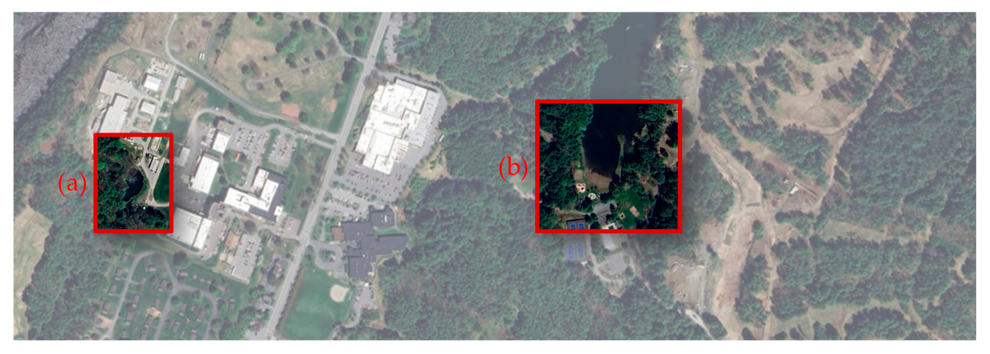
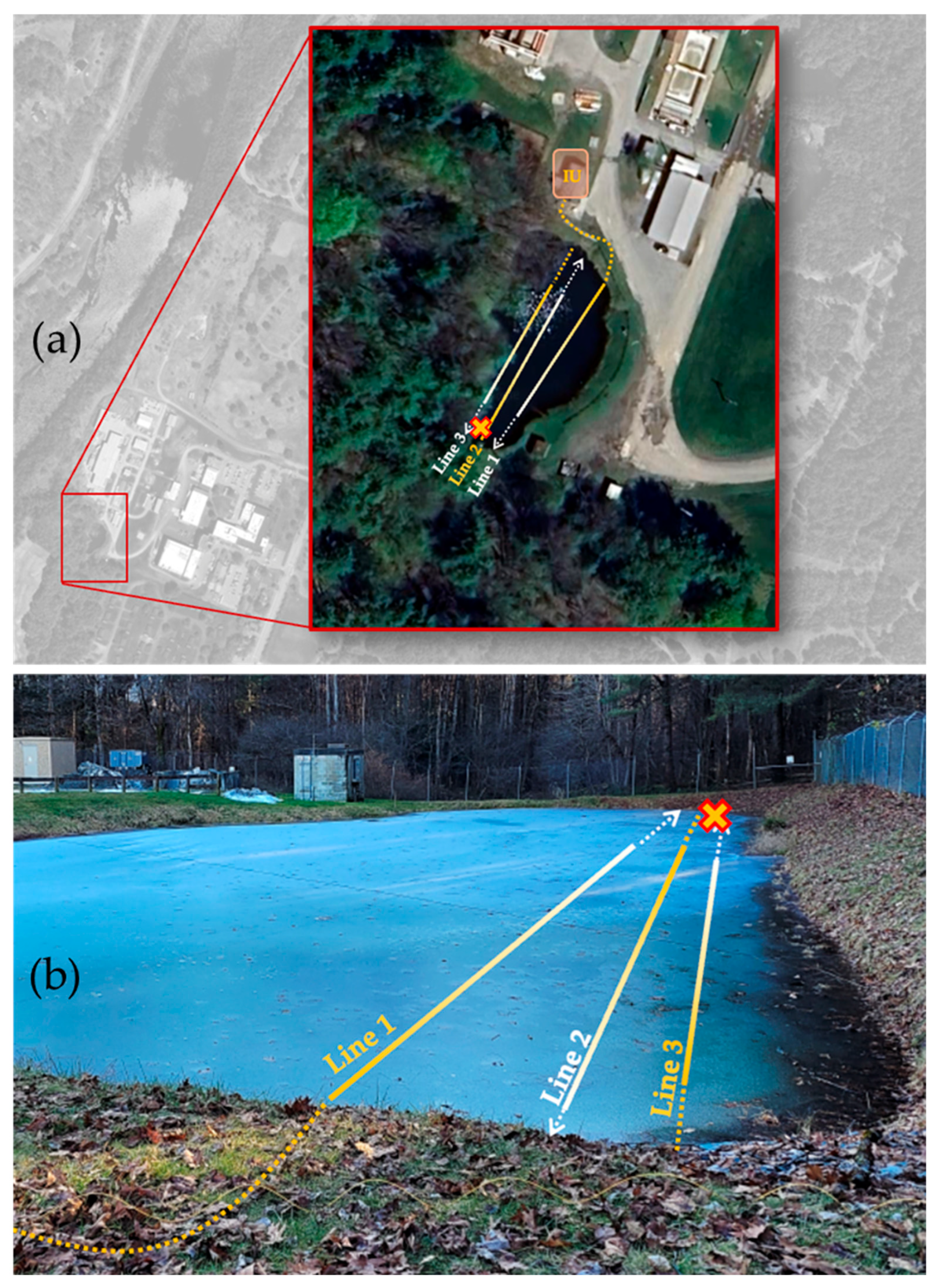
2.1. Phase 1: CRREL Pond

The first phase, a pilot study, occurred on the CRREL campus in December 2023. After a week of −11 °C to 10 °C temperatures, a thin ice sheet developed on the freshwater pond (approximately 55 m by 30 m by about 1 m deep). The day prior to DAS data collection, a lightweight, urethane-jacketed simplex single-mode fiber optic cable was deployed on the thin ice sheet without trespassing on the ice sheet. To accomplish this, our team unspooled the fiber on the bank of the pond and carried the fiber line to the desired position. The IU was connected to the fiber in a small facility with power on the north end of the pond. Figure 2 shows the cable layout. Temperatures ranged from −5 °C to 5 °C on the day of cable deployment. The cable froze into the thin ice overnight, and data collection proceeded the following day with temperatures ranging from −3 °C to 4 °C. Freeze-in depth was not measured in situ, but the entirety of the fiber (0.2 cm diameter) was encased in the ice. The ice sheet was thin, extending to the pond perimeter overnight and melting around the edges during the day under the sun.

A Sintela Onyx phase-sensitive DAS interrogator recorded with a gauge length of 3.2 m, channel spacing of 1.6 m, and sampling frequency of 2500 Hz. The length of the fiber optic cable was measured to be 2500 m, with about 520 m installed near and on the ice. The data was 32 BIT raw. A GPS time sync module connected to the IU kept accurate time. Due to the thinness of the ice, strikes were performed from shore using a 5 cm diameter, 150 cm long metal pipe. Figure 2 shows the location of the strikes analyzed herein, indicated by the “X” marker.

The research team analyzed the DAS data using the phase velocity transform described by Park et al. [12] to obtain a characteristic dispersion curve of the thin ice sheet in the phase velocity–frequency domain. Nziengui-Ba et al. [17] indicated that the seismic wavefield of a vibration source exciting a sheet of floating ice can be described by three fundamental acoustic modes: a non-dispersive, longitudinal wave; a non-dispersive, horizontal shear wave; and a Quasi-Scholte, ice flexural wave. The non-dispersive, longitudinal wave (similar to a compression wave) and the non-dispersive, horizontal shear wave may provide information about the ice properties, but do not correlate to ice thickness measurements. However, Quasi-Scholte flexural waves, with particle motion similar to a Rayleigh wave on land, are dispersive and provide useful information for ice thickness estimations. Phase velocity data was interpreted along Lines 1 and 2 in this study. Line 3 initiated several meters away from the strike location. Interpretation of data along Line 3 with an inaccurate estimate of the angle of propagation could bias wave speed estimates low along this line.

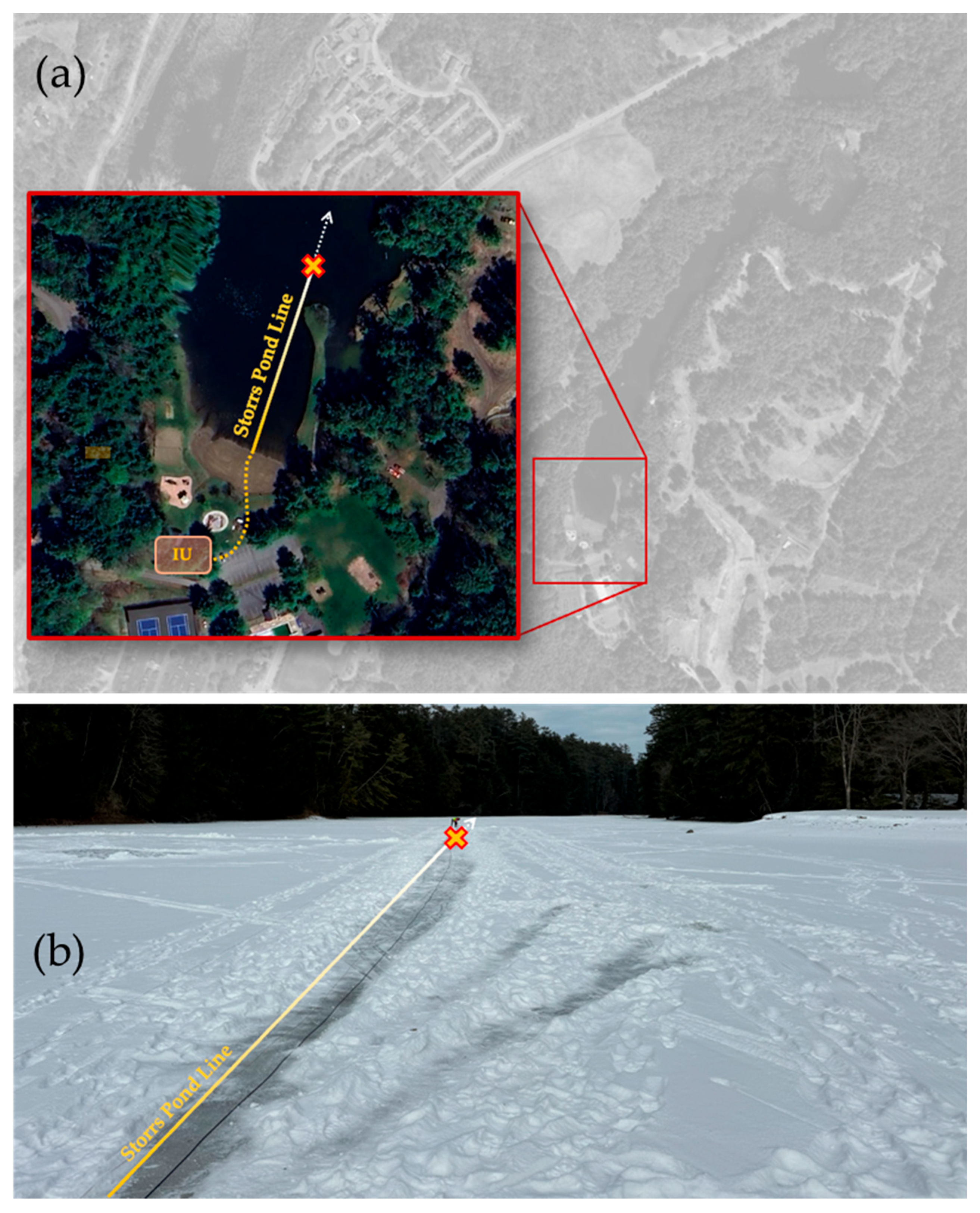
2.2. Phase 2: Storrs Pond

With pilot test validation, a follow up field study was performed at Storrs Pond in January 2025 to further explore the potential of surface-deployed DAS to measure dispersive waves on a larger ice sheet. In the week leading up to the experiment, the mean temperature was −9 °C in the Storrs Pond area. On the day of testing, temperatures ranged from −3 °C to 13 °C. Approximately 10 cm of snow was shoveled from the ice surface in a 100 m straight line from the shore towards the center of the pond. The cable, a Silixa tactical fiber optic cable with 2 m Constellation optical fiber, rated for −55 °C with an outer diameter of 5.5 mm, was rapidly deployed and laid directly atop the ice. The ice thickness along the cable deployment measured to be between 25.5 and 28 cm per hand augering.

A Silixa iDAS Carina IU recorded with a gauge length of 2 m, channel spacing of 0.25 m, and sampling frequency of 5000 Hz. Of the 500 m long cable, about 100 m was installed on the ice. The data was saved in TDMS format. A GPS time sync module kept accurate time. A calibrated drop hammer (a proctor hammer) striking a metal plate was used as a seismic source in this test. Figure 3 shows the location of the impacts (indicated by the “X” marker) analyzed herein.

3. Results

3.1. CRREL Pond

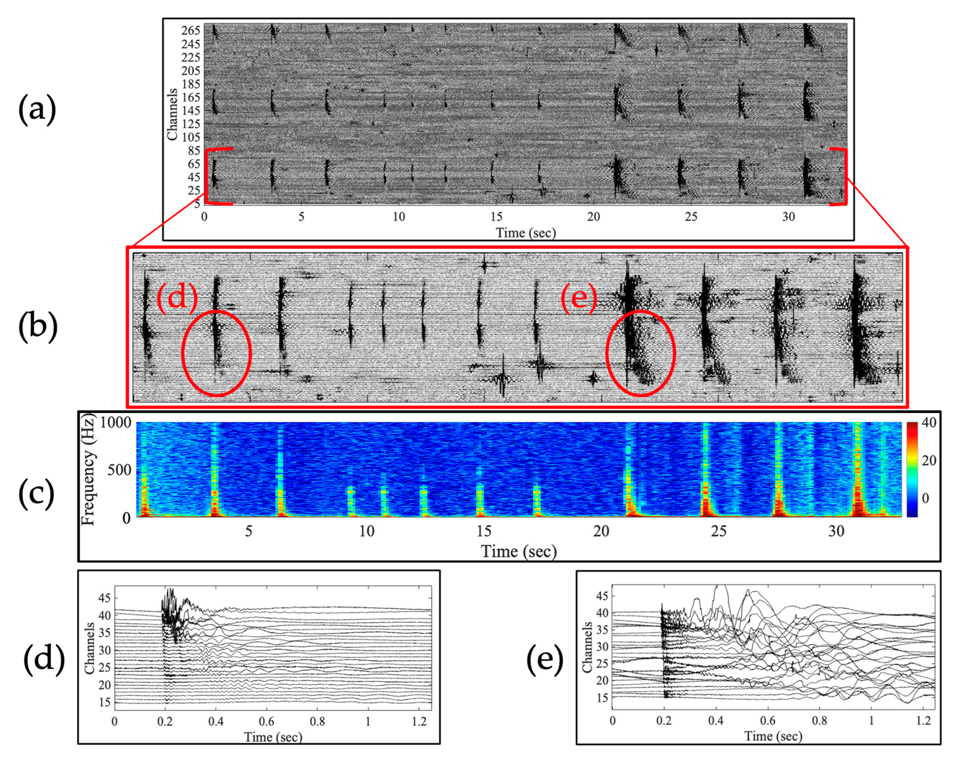
3.1.1. Initial Waveform Analysis

An example of the response of the Sintela DAS to impact strikes is shown in Figure 4. In this example, 12 strikes are observed along three sub-parallel portions of the fiber optic cable. The responses show the impact of variable (uncalibrated) impact strength, with the last four strikes (seconds 20–34) resulting in ice failure. The amplitude of the spectrogram, along with the highest frequencies excited, correspond with the strength of the impact strikes.

3.1.2. Dispersion Modeling

To model flexural wave speeds, the methodology of Nziengui-Ba et al. [17], Romeyn et al. [19], and Stein et al. [20] was followed, whereby the longitudinal wavenumber (k_QS0) and the flexural wavenumber (k_QS) are given as:

$$k_{QS0}=\omega \sqrt{{\displaystyle \frac{\rho \left(1-{\mathsf{\nu }}^2\right)}{E}}}$$

(1)

$$D\left(h\right){\displaystyle \frac{k_{QS}^5}{{\rho }_w}}+g{k}_{QS}={\mathsf{\omega }}^2\left[k_{QS}h{\displaystyle \frac{{\rho }_w}{\rho }}+\cot \mathrm{h}\left(k_{QS}H\right)\right]$$

(2)

$$D\left(h\right)={\displaystyle \frac{E{h}^3}{12\left(1-{\mathsf{\nu }}^2\right)}}$$

(3)

In these equations, ω is angular frequency, ρ is ice density, ν is Poisson’s ratio of the ice, E is Young’s modulus of the ice, D(h) is ice bending rigidity, g is gravitational acceleration, h is ice thickness, ρ_w is water density, and H is the depth of the water column below the floating ice. Through these coupled equations, properties of interest (here, ice thickness and density) were recovered through measurements of non-dispersive longitudinal wave speeds and dispersive flexural wave speeds.

Modeling of flexural wave dispersion over a thin ice sheet suggests that phase velocities should increase with increasing frequency. A baseline model was developed in which ice thickness (h) was assumed to be 5 cm, pond depth (H) was assumed to be 1.0 m based on knowledge of the site, Poisson’s ratio (ν) was assumed to be 0.30, the density of ice (ρ_ice) was assumed to be 0.915 g/cc, and the density of water (ρ_w) was assumed to be 1.000 g/cc. A sensitivity analysis was performed to quantify the relative sensitivities of the flexural wave phase velocities due to incremental changes in mechanical properties. The results indicate that 5% increases in density, compressional velocity, and thickness yielded increases of 7%, 15%, and 22%, respectively, across the frequencies of interest here (Figure 5; 10–52 Hz was modeled, and only computations for 40–52 Hz are shown). To support missions ensuring safety on public waterways with thin ice sheets, the research focused on assessing significant variations in ice thickness. Therefore, throughout this analysis, simplified assumptions were made about other variables to focus on constraining the thickness of the ice across the pond. No variation in ice thickness (or other properties) was assumed along the DAS line, nor for the fixed pond depth, Poisson’s ratio, the density of ice, and the density of water in our model calculations. Quantification of ice properties along cable changes would be a valuable extension of this work.

3.1.3. Longitudinal and Flexural Wave Analysis

Wave speed analysis was performed on Lines 1 and 2 of the array. Along Line 1, the velocity of the longitudinal wave was measured to be 3248 ± 10 m/s, which is somewhat below the published compressional velocity of pure ice values of 3400–3800 m/s [21]. Lower compressional velocities than those of pure ice, as observed here, are consistent with impurities in the ice, which were observed but not quantified in situ during our study.

The phase velocities of the flexural waves were measured using a phase velocity transformation. Within this methodology, the phase velocity which gives the highest-power beamformed output is selected as a function of frequency; refer to Park et al. [12] for more details. An example of the calculations along Line 1 is shown in Figure 6. While coherent noise appears present at many frequencies, a clear amplitude peak showing increasing phase velocity with increasing frequency can be observed. This trend is typical of flexural waves, though an inverse trend is typical of Rayleigh waves in the solid Earth with increasing seismic velocities with depth [22].

3.1.4. Ice Thickness Estimation

While generating models for phase velocity as a function of frequency for different ice thickness values, measurements for longitudinal wave velocity were used to constrain the Young’s modulus. As demonstrated during the sensitivity analysis, the phase velocities are sensitive to all these parameters, but the interest of this research is in determining ice thickness, which varies by orders of magnitude more than the other parameters.

The flexural wave phase velocities along Lines 1 and 2 are shown in Figure 7. To produce each curve, the phase velocities along each line following strikes 1, 2, and 3 were estimated. The values presented in Figure 7 represent the mean and standard deviation of the measurements as a function of frequency. Lower velocities were measured along the edge of the pond, suggesting that ice thins near the edge; modeling (also shown in Figure 7) suggests that the ice thickness thins from 5 cm to 3.5 cm between Lines 1 and 2. The near-shore thickness was confirmed in situ. At the perimeter of the pond, the ice thickness reduced to nothing.

3.2. Storrs Pond

3.2.1. Longitudinal and Flexural Wave Analysis

An example of the response of the Silixa IU to proctor hammer strikes is shown in Figure 8. In this example, five strikes are observed along the array, originating from the furthest portion of the array (~Channel 640) and propagating along the ice sheet. The strikes are consistent in amplitude and frequency content, which pairs well with the use of the calibrated proctor hammer source. The amplitude of the spectrogram, along with the highest frequencies excited, correspond with the strength of the impact strikes.

Analysis of wave speeds was performed along the single deployed length of the array. The velocity of the longitudinal wave was measured to be approximately 3220 m/s. Phase velocities of the flexural waves were measured using the Frequency Domain Beamformer transformation [23] considering the second, third, and fourth strikes in the proctor hammer strike sequence. Three strikes were selected for wave speed analysis to maintain consistency with the methodology of the first field effort.

3.2.2. Ice Thickness Estimation

Direct measurements of ice thickness and water depth helped constrain and reduce error in the theoretical modeling. Model parameters were kept constant from the CRREL pond calculations, with the only deviation being that water depth was instead fixed at H = 2.0 m. The flexural wave phase velocities along the Storrs Pond line are shown in Figure 9, where the values represent the mean and standard deviation of the three measurements as a function of frequency. Direct measurements of the ice thickness, via auger holes and a tape measure, indicated that ice along the array varied between 25.5 and 28 cm. In validation, the flexural wave dispersion measurements fit a curve situated between the theoretical curves for these values.

4. Discussion

Historically, lake ice formation characterization has been spatially limited by surveys using a discrete number of in situ point measurements [24]. In recent years, remote sensing techniques have expanded lake ice dynamics spatial measurement capabilities [24]; however, ground truthing and model validation typically still use limited point measurements [24,25]. This study demonstrates that DAS can be effectively used for the estimation of spatially variable ice thickness of a thin ice sheet on a freshwater pond, laying the groundwork to monitor larger thin ice sheets on freshwater bodies. Large-scale, stand-off monitoring of thin ice sheets with high spatial resolution will provide additional insight into ice formation, ice evolution through time, and the transport of freshwater resources through cold watersheds.

Researchers are studying driving factors and trends of freshwater ice thickness variation in North America [26]. In a separate study, researchers assessed the ice quality (which has implications on strength and thickness) of lake ice during a warm winter and found an increase in white ice [27], which can have safety implications. Mapping, monitoring, and measuring ice thickness and ice properties using DAS would allow for stand-off risk assessments of ice sheets and contribute to our understanding of thin ice sheets on freshwater bodies. From a protected, sheltered location, operational assessment of ice thickness could be performed to spatially evaluate and monitor ice thickness safety concerns. Providing near-real-time ice thickness estimates would in turn allow for the determination of safe loading locations with potential for rapid-response monitoring and action. Similarly, the dynamic capabilities of DAS monitoring systems would allow for the detection and localization of bending, fracture, and cracking activity in ice as well as the assessment of other dynamic properties.

The analysis presented here leverages the relative homogeneity of the test ponds, with a near-constant water depth (approximately 1 m in the CRREL pond and 2 m in Storrs Pond) to simplify the analyses and modeling. In many real-world applications, the variable depth of the water beneath the fiber optic cable for ice monitoring purpose will need to be known a priori (or solved for) to provide accurate estimates. Simplifying assumptions about ice density, water density, Poisson’s ratio, and other parameters (i.e., the assumption that wave speed is invariant) may not be valid for other environments. Future work will evaluate the ability of DAS testing to estimate changes in ice thickness across the length of the fiber optic cable. With sufficiently high spatial resolution and sampling rate, along-fiber variations in wave speeds’ (and therefore ice properties’) spatial difference could be interrogated and mapped.

For these studies, the fiber optic cables were rapidly deployed on the surface in approximately one hour. It is also possible to install the fiber optic cable in ice [1,5] or to potentially grow the cable into ice. Having a cable or cable layers within an ice sheet would provide a unique look at the inner mechanics of ice spatially in three dimensions with the ability to monitor both static and dynamic conditions. Studying ice growth and ice cycles with DAS complements existing efforts at microscopic and macroscopic scales.

5. Conclusions

This study demonstrates the feasibility of using DAS to monitor spatially variable ice properties, such as thickness, in areas that may be unsafe for human traffic or direct sampling. This research is an initial step towards advancing and expanding the use of DAS to spatially measure and monitor large-scale freshwater bodies at high spatial resolution. As this application of DAS matures, it will provide important safety information for risk assessments along with high-resolution, continuous monitoring and a deeper understanding of ice static and dynamic mechanics.

References

1. Quinn, M.C.L.; Wagner, A.M.; Engel, C.S.; Winters, K.E.; Coclin, C.G.; Picucci, J.R. Distributed Fiber Optic Sensing in Cold Regions. In Proceedings of the Geo-Congress 2024, Vancouver, BC, Canada, 25–28 February 2024; pp. 536–544. [Google Scholar]
2. Glaser, D.R.; Costley, R.D.; Hathaway, K.; Boitnott, G.; Weale, J. Snow Coupled Distributed Acoustic Sensing for Intrusion Detection of Polar Bears in Arctic Camps. In Proceedings of the Symposium on the Application of Geophysics to Engineering and Environmental Problems 2021, Online Conference, 11 June 2021; p. 262. [Google Scholar]
3. Lindsey, N.J.; Rademacher, H.; Ajo-Franklin, J.B. On the Broadband Instrument Response of Fiber-Optic DAS Arrays. JGR Solid Earth 2020, 125, e2019JB018145. [Google Scholar] [CrossRef]
4. Soga, K.; Luo, L. Distributed Fiber Optics Sensors for Civil Engineering Infrastructure Sensing. J. Struct. Integr. Maint. 2018, 3, 1–21. [Google Scholar] [CrossRef]
5. Quinn, M.C.L.; Flynn, D.; Engel, C.; Potty, G.R.; Coclin, C.G.; Baxter, C.D.P. Distributed Acoustic Sensing (DAS) in Ice. In Proceedings of the Underwater Acoustics Conference and Exhibit, Kalamata, Greece, 25–30 June 2023. [Google Scholar]
6. Walter, F.; Gräff, D.; Lindner, F.; Paitz, P.; Köpfli, M.; Chmiel, M.; Fichtner, A. Distributed Acoustic Sensing of Microseismic Sources and Wave Propagation in Glaciated Terrain. Nat. Commun. 2020, 11, 2436. [Google Scholar] [CrossRef] [PubMed]
7. Booth, A.D.; Christoffersen, P.; Schoonman, C.; Clarke, A.; Hubbard, B.; Law, R.; Doyle, S.H.; Chudley, T.R.; Chalari, A. Distributed Acoustic Sensing of Seismic Properties in a Borehole Drilled on a Fast-Flowing Greenlandic Outlet Glacier. Geophys. Res. Lett. 2020, 47, e2020GL088148. [Google Scholar] [CrossRef]
8. Fichtner, A.; Hofstede, C.; Gebraad, L.; Zunino, A.; Zigone, D.; Eisen, O. Borehole Fibre-Optic Seismology inside the Northeast Greenland Ice Stream. Geophys. J. Int. 2023, 235, 2430–2441. [Google Scholar] [CrossRef]
9. Hudson, T.S.; Baird, A.F.; Kendall, J.M.; Kufner, S.K.; Brisbourne, A.M.; Smith, A.M.; Butcher, A.; Chalari, A.; Clarke, A. Distributed Acoustic Sensing (DAS) for Natural Microseismicity Studies: A Case Study from Antarctica. JGR Solid Earth 2021, 126, e2020JB021493. [Google Scholar] [CrossRef]
10. Xie, J.; Zeng, X.; Liang, C.; Ni, S.; Chu, R.; Bao, F.; Lin, R.; Chi, B.; Lv, H. Ice Plate Deformation and Cracking Revealed by an in Situ-Distributed Acoustic Sensing Array. Cryosphere 2024, 18, 837–847. [Google Scholar] [CrossRef]
11. Peña Castro, A.F.; Schmandt, B.; Baker, M.G.; Abbott, R.E. Tracking Local Sea Ice Extent in the Beaufort Sea Using Distributed Acoustic Sensing and Machine Learning. Seism. Rec. 2023, 3, 200–209. [Google Scholar] [CrossRef]
12. Park, C.B.; Miller, R.D.; Xia, J. Imaging dispersion curves of surface waves on multi-channel record. SEG Tech. Program Expand. Abstr. 1998, 1377–1380. [Google Scholar] [CrossRef]
13. Mateeva, A.; Lopez, J.; Potters, H.; Mestayer, J.; Cox, B.; Kiyashchenko, D.; Wills, P.; Grandi, S.; Hornman, K.; Kuvshinov, B.; et al. Distributed Acoustic Sensing for Reservoir Monitoring with Vertical Seismic Profiling. Geophys. Prospect. 2014, 62, 679–692. [Google Scholar] [CrossRef]
14. Dean, T.; Cuny, T.; Hartog, A.H. The Effect of Gauge Length on Axially Incident P-waves Measured Using Fibre Optic Distributed Vibration Sensing. Geophys. Prospect. 2017, 65, 184–193. [Google Scholar] [CrossRef]
15. Daley, T.M.; Miller, D.E.; Dodds, K.; Cook, P.; Freifeld, B.M. Field Testing of Modular Borehole Monitoring with Simultaneous Distributed Acoustic Sensing and Geophone Vertical Seismic Profiles at Citronelle, Alabama. Geophys. Prospect. 2016, 64, 1318–1334. [Google Scholar] [CrossRef]
16. Harmon, N.; Rychert, C.A.; Davis, J.; Brambilla, G.; Buffet, W.; Chichester, B.; Dai, Y.; Bogiatzis, P.; Snook, J.; Van Putten, L.; et al. Surface Deployment of DAS Systems: Coupling Strategies and Comparisons to Geophone Data. Near Surf. Geophys. 2022, 20, 465–477. [Google Scholar] [CrossRef]
17. Nziengui-Bâ, D.; Coutant, O.; Moreau, L.; Boué, P. Measuring the Thickness and Young’s Modulus of the Ice Pack with DAS, a Test Case on a Frozen Mountain Lake. Geophys. J. Int. 2023, 233, 1166–1177. [Google Scholar] [CrossRef]
18. Department of the Army. Engineering and Design: Ice Engineering. In US Army Corps of Engineers, Engineer Manual 1110-2-1612; USACE: Washington, DC, USA, 2022; p. 475. [Google Scholar]
19. Romeyn, R.; Hanssen, A.; Ruud, B.O.; Johansen, T.A. Sea Ice Thickness from Air-Coupled Flexural Waves. Cryosphere 2021, 15, 2939–2955. [Google Scholar] [CrossRef]
20. Stein, P.J.; Euerle, S.E.; Parinella, J.C. Inversion of Pack Ice Elastic Wave Data to Obtain Ice Physical Properties. J. Geophys. Res. 1998, 103, 21783–21793. [Google Scholar] [CrossRef]
21. Jin, B.; Lianhui, J.; Chunxia, M.; Fengrui, B. Test and Analysis of Compression Wave Sound Velocity Measurement in Ice by Direct Method. In Proceedings of the 2021 OES China Ocean Acoustics (COA), Harbin, China, 14–17 July 2021; pp. 1095–1099. [Google Scholar]
22. Aki, G.C.; Richards, P.G. Quantitative Seismology, Theory and Methods. Geol. Mag. 1981, 118, 208. [Google Scholar] [CrossRef]
23. Zywicki, D.J.; Rix, G.J. Mitigation of Near-Field Effects for Seismic Surface Wave Velocity Estimation with Cylindrical Beamformers. J. Geotech. Geoenviron. Eng. 2005, 131, 970–977. [Google Scholar] [CrossRef]
24. Murfitt, J.; Duguay, C.R. 50 Years of Lake Ice Research from Active Microwave Remote Sensing: Progress and Prospects. Remote Sens. Environ. 2021, 264, 112616. [Google Scholar] [CrossRef]
25. Brown, L.C.; Duguay, C.R. A Comparison of Simulated and Measured Lake Ice Thickness Using a Shallow Water Ice Profiler. Hydrol. Process. 2011, 25, 2932–2941. [Google Scholar] [CrossRef]
26. Imrit, M.A.; Yousaf, Z.; Sharma, S. Quantifying the Trends and Drivers of Ice Thickness in Lakes and Rivers across North America. Water 2022, 14, 1841. [Google Scholar] [CrossRef]
27. Weyhenmeyer, G.A.; Obertegger, U.; Rudebeck, H.; Jakobsson, E.; Jansen, J.; Zdorovennova, G.; Bansal, S.; Block, B.D.; Carey, C.C.; Doubek, J.P.; et al. Towards Critical White Ice Conditions in Lakes under Global Warming. Nat. Commun. 2022, 13, 4974. [Google Scholar] [CrossRef] [PubMed]
Figure 1. Location and size of the two freshwater bodies discussed in this paper, where (a) is the CRREL pond and (b) is Storrs Pond. (Airbus Imagery from the date: 5 July 2024).
Glacies 02 00007 g001
Figure 2. (a) Aerial view of the CRREL pond indicating cable layout. Airbus Imagery from the date: 5 July 2024. (b) Photo of the study site (CRREL campus, Hanover, NH, USA) with approximate locations of the fiber optic cable lengths considered in this analysis. The “X” marker represents the location of the ice strikes at the south end of the pond. For scale, the pond is 55 m north to south and 30 m east to west.
Glacies 02 00007 g002
Figure 3. (a) Aerial view of Storrs Pond showing cable layout. Airbus Imagery from the date: 5 July 2024. (b) Photo of the study site (Storrs Pond, Hanover, NH, USA) with approximate location of the fiber optic cable length considered in this analysis. The “X” marker represents the location of the impacts.
Glacies 02 00007 g003
Figure 4. Waveform data recorded by the Sintela IU following a set of 12 strikes on the ice. Data were high-pass-filtered with a cutoff frequency of 2 Hz. (a) A 34 s record of the DAS measurements showing time on the horizontal axis and channel number on the vertical axis. Note that the taps appear in three distinct locations, corresponding to Lines 1–3. (b) A zoom-in on the strikes along Line 1. (c) A spectrogram of the strikes recorded at Channel 28 (Line 1) The amplitude is shown as dB re: counts. (d) A further zoom-in on strike 2. (e) A further zoom-in on strike 9.
Glacies 02 00007 g004
Figure 5. Sensitivity of the flexural wave phase velocities as given by our forward model. The “baseline” model corresponds to our 5 cm ice thickness model described in the text. For each perturbation, the parameter was varied by 5%.
Glacies 02 00007 g005
Figure 6. Normalized amplitude (varying between 0 and 1) as a function of phase velocity and frequency following strike 2 along Line 1. Estimates of the flexural wave phase velocities are shown by the red dots.
Glacies 02 00007 g006
Figure 7. Phase velocity as a function of frequency for Line 1 (blue) and Line 2 (green). Modeled phase velocities corresponding to 2.5 cm, 5 cm, and 7.5 cm of ice are shown in the dashed lines.
Glacies 02 00007 g007
Figure 8. Waveform data recorded by the Silixa IU following a set of 5 proctor hammer strikes on the ice at Storrs Pond. Data were high-pass-filtered with a cutoff frequency of 2 Hz. (a) A 17 s record of the DAS measurements showing time on the horizontal axis and channel number on the vertical axis. (b) A spectrogram of the strikes recorded at Channel 510. The amplitude is shown as dB re: counts. (c) A further zoom-in on the second strike in the sequence.
Glacies 02 00007 g008
Figure 9. Phase velocity as a function of frequency for the Storrs Pond line (red). Modeled phase velocities corresponding to 25 cm and 28 cm of ice are shown in the dashed lines.
Glacies 02 00007 g009
Disclaimer/Publisher’s Note: The statements, opinions and data contained in all publications are solely those of the individual author(s) and contributor(s) and not of MDPI and/or the editor(s). MDPI and/or the editor(s) disclaim responsibility for any injury to people or property resulting from any ideas, methods, instructions or products referred to in the content.