Article

Surface Water Extent Extraction in Prairie Environments Using Sentinel-1 Image-Pair Coherence

Department of Geography and Environmental Management, University of Waterloo, Waterloo, ON N2L 3G1, Canada
*
Author to whom correspondence should be addressed.
Submission received: 18 December 2024 / Revised: 27 March 2025 / Accepted: 1 April 2025 / Published: 19 May 2025

Abstract

:
Knowledge of surface water extent is critical for ecological and disaster monitoring. However, surface water extraction from optical satellite imagery is challenging due to the impact of weather. Synthetic Aperture Radar (SAR) can penetrate cloud cover and has significant advantages for surface water mapping, but the classification accuracy might be limited by SAR’s inherent properties and land cover, which have similar backscatter to surface water. This study finds that the accuracy of surface water extraction at the Prairie Pothole Region (PPR) can be improved by combining interferometric coherence and backscatter for machine learning classification. This study performs time-series analysis on surface water and land to investigate their discrimination at different seasonal periods. The accuracy improvement of this method on Sentinel-1 images reached 10% during the seasons of fall and winter, where the combination of backscatter and coherence was proven to be efficient for separating water and land. Hence, our approaches of combining backscatter and coherence provide new insights for surface water extraction from SAR images in future studies.

1. Introduction

Surface water, including lakes and rivers, is inherently dynamic, undergoing fluctuations in size, shape, and course over time due to a variety of natural, seasonal, and human-influenced factors [1,2]. The current shift in climate patterns is introducing significant alterations to surface water dynamics, including changes in water levels and extents, shifts in lake distributions, and the complete disappearance of lakes in some cases [3]. Therefore, it is imperative to precisely monitor these dynamic changes to effectively conserve and manage surface water resources. Surface water constitutes a crucial component of terrestrial water storage (TWS), with its fluctuations playing a pivotal role in the TWS climatology of terrestrial ecosystems [4,5]. The accurate estimation of surface water is vital as it impacts the retrieval of groundwater using TWS data from satellite observations such as the Gravity Recovery and Climate Experiment (GRACE). Furthermore, surface water coverage directly regulates evaporative water loss from inland water bodies within terrestrial ecosystems, influencing the ecosystem’s water budget [6,7,8]. It also plays a crucial role in the land surface energy budget due to its low albedo [9]. Given these considerations, the continuous monitoring of surface water is paramount for advancing water resource management and climate research.
Satellite imagery plays a crucial role in detecting and monitoring surface water in remote regions of Canada [10]. Currently, optical instruments such as the Moderate-Resolution Imaging Spectroradiometer (MODIS), Landsat missions, and Sentinel-2 missions have been extensively studied for surface water monitoring [11,12,13,14]. The multispectral properties of optical sensors offer significant advantages in surface water extraction. For instance, several studies have utilized multispectral information to compute water indices like the Normalized Difference Water Index (NDWI), the enhanced water index (EWI), and the Modified Normalized Difference Water Index (MNDWI) for surface water extraction [10,13,14,15,16,17]. However, the efficacy of optical remote sensing may be hampered by factors such as clouds, atmospheric effects, and other environmental conditions, which could hinder the continuous monitoring of surface water.
Alternatively, active microwave sensors such as Synthetic Aperture Radar (SAR) can penetrate clouds and detect earth surfaces without solar radiation, making it an all-weather sensor [18]. Several surface water extraction studies have used SAR imagery because smooth and open water causes the specular reflection of the incoming signal, resulting in lower backscatter coefficients relative to land [12,18,19,20]. However, the surface roughness of water is dependent on whether or not wind is present; Bragg scattering results in higher backscatter signals caused by winds and waves, which lowers the separability of backscatter between water and land [12,20,21]. Previous studies have concluded that co-polarization data (HH and VV) are more affected by water surface roughness [19,22] compared to cross-polarized (VH and HV) imagery [12,22]. Different levels of incidence angle can also result in changes in the contrast of backscatter signals between water and land, which influences the accuracy of surface water extraction [12,20,23]. During cold seasons, the surface water can be frozen, and the lake ice formation, cracks, and deformation may result in an increase in backscatter, which might result in similar backscatter properties between frozen surface water and land [24]; the increase in backscatter might also come from increased roughness at the lake ice–water interface [25]. However, the backscatter is decreased if the surface water is frozen to the lake bed where the radar signal penetrates through the ice cover and interacts with the ground surface [25]. In addition, sandy surfaces, dry land, and wet snow cover might lead to a decrease in backscatter that can be confused with surface water [26,27,28]. For the agricultural land cover, the backscatter of crops during the growing season is distinguishable from surface water, but it decreases after the harvest period, which might lead to similar backscatter properties to surface water [29]. Short grass has lower backscatter during dry seasons as vegetated canopies do not exist in these areas [30]. Hence, limitations exist for surface water extraction using SAR backscatter as an image classification feature where the backscatter characteristic of surface water and land might be similar in some scenarios.
Phase information using the SAR system may be useful for surface water monitoring and discriminating surface water from other land cover types. The technique using change in the observed phase of the target is known as Interferometric SAR (InSAR) and is widely applied in change detection for agricultural growth monitoring, flooding detection, surface deformation, and wetland mapping [9,29,31,32]. The coherence information can be derived by using the InSAR technique by accessing two SAR images with different spatial or temporal baselines [33]. The coherence parameter represents the consistency of surface properties’ interaction with radar waves at the same location between two acquisitions [34,35,36]. Coherence information from InSAR may provide valuable information for surface water mapping since the scattering properties of surface water are more likely to change over a short period with waves caused by the wind, which leads to a decrease in coherence [32,37,38]. When surface water is frozen, the growth of the ice surface towards the bottom of the waterbody will continually change the ice–water interface and therefore still maintain low coherence [39]. However, if the overlying ice cover is of sufficient thickness to freeze to the lakebed, the coherence might be increased due to the thickness not changing significantly [39]. Hence, the InSAR coherence of surface water can be considered to be consistently low at most temporal periods, which should be explored to improve the accuracy of surface water mapping [37].
For agricultural croplands, the coherence value has been shown to be correlated to the stage of crop growth. Generally, the coherence is lower during the crop growing period and increases after the harvest season when the underlying soil is a consistent target [29,40], which might provide additional information to help separate agricultural land and surface water. Coherence for agricultural land may also be consistently high before plowing and after sowing until crop emergence [29]. Additionally, short grassland areas can maintain higher coherence because canopy structures do not exist in short grass, where the grass structure is less affected by wind [41,42,43]. When the land surface is covered by snow, the coherence of land is inversely related to changes in snow depth [44]. In summary, the use of InSAR coherence shows potential to improve the accuracy of surface water extraction without incorporating multiple datasets and wavelengths.
Supervised machine learning algorithms from earth observation data have been widely used in surface water detection and monitoring [23,27,45,46,47,48,49]. Machine learning classification methods can combine backscatter features from SAR imagery for surface water classification, which can improve classification accuracy [23,46,50]. Additionally, backscatter features can be combined with coherence information to optimize the classification result [51,52,53,54,55]. However, supervised classification requires a prepared training set as classification accuracy is also affected by the training set; the preparation process of the training set is expensive and time-consuming. Recently, multiple studies adopted the process of automatically selecting training samples from historical surface water datasets [11,14,23,27,49]. Available surface water datasets included a Landsat-based global surface water (GSW) dataset with 30 m spatial resolution, generated by the Joint Research Center (JRC) and retrieved from Landsat observations [1]. The dataset was further improved to develop a more accurate surface water base map (SWB), including permanent surface water, permanent land, and water occurrences, in Canada for the period of 1991 to 2020 [2].
Although multiple studies identify InSAR coherence as a source of improvement for water extraction, there is a lack of studies incorporating it in surface water mapping products [27,32,37]. This study will investigate how the coherence information for multiple temporal baselines can be exploited to improve surface water extent retrievals in the Prairie Pothole Region of Saskatchewan, Canada. Specifically, the objectives of this research are to (1) derive coherence information from 2019 to 2023 every month using a 12-day temporal baseline and every winter period between November and February using a 24-day temporal baseline; (2) use the derived coherence to perform time-series analysis with ground truth data to investigate the seasonal change in coherence value between surface water and land; and (3) use coherence and backscatter information as the input to a machine learning algorithm to quantify the accuracy improvement using coherence information at different seasonal periods.

2. Materials and Methods
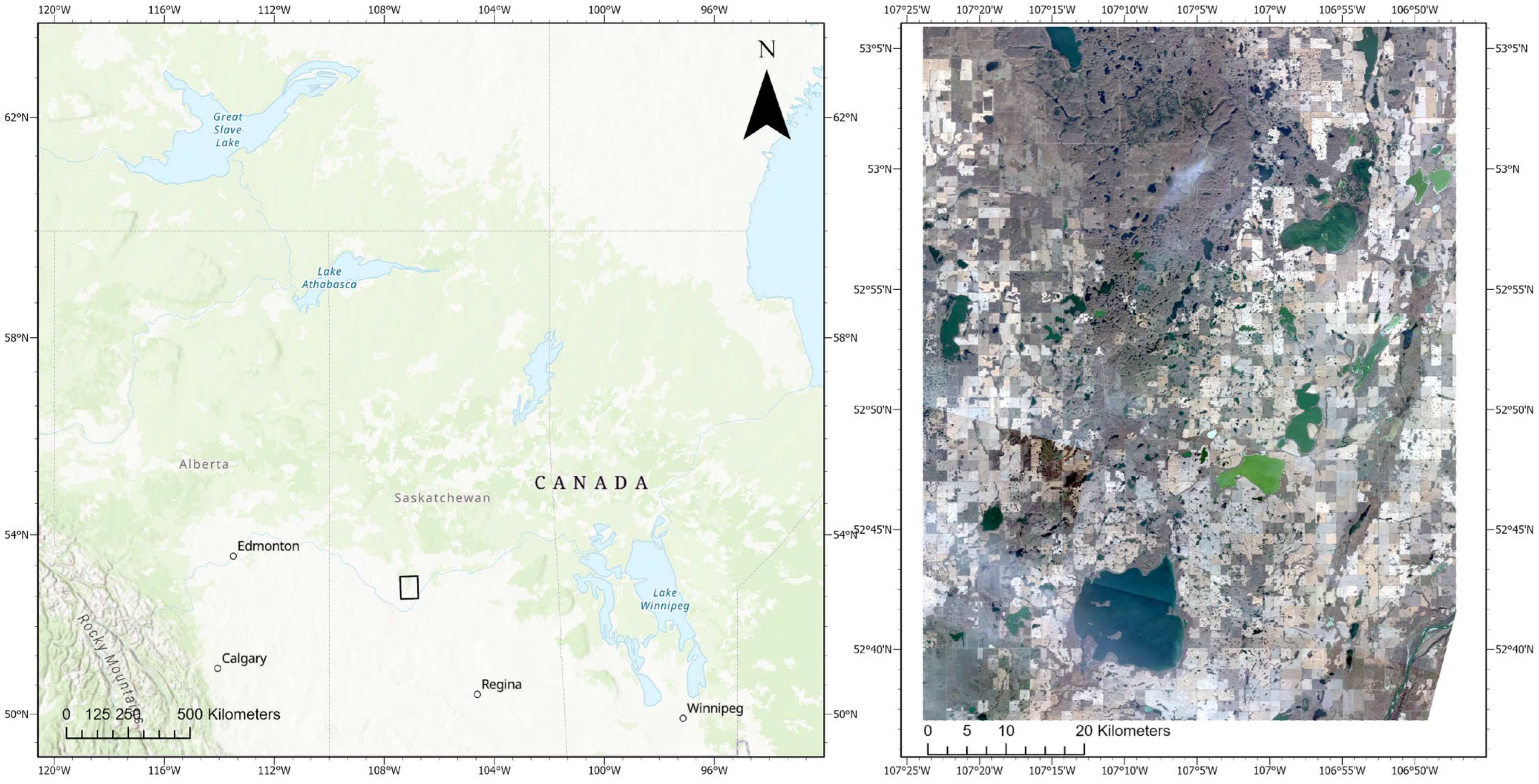
2.1. Study Area

The Prairie Pothole Region (PPR) encompasses the southern reaches of the Canadian provinces of Alberta, Saskatchewan, and Manitoba, alongside various states stretching from Iowa to the Dakotas in the United States, including a vast expanse totaling approximately 777,000 km2 [56]. These distinctive potholed landscapes owe their existence to the retreating glaciers at the culmination of the last glacial epoch, a pivotal event in the region’s geological history [57], integral to its hydrological dynamics [58]. For the agricultural land cover, the backscatter of crops during the growing season is distinguishable from surface water, but it decreases after the harvest period, which might lead to similar backscatter properties as surface water [29]. The surface water dynamics within the PPR exhibit a profound sensitivity to both climatic fluctuations and seasonal variability [3,30,59].
The focus of this study encompasses Redburry lake, situated northwest of Saskatoon and within the Prairie Pothole Region (PPR) (Figure 1). This region is selected as the study site due to its diverse landcover, containing lakes, potholes, rivers, wetlands, cropland, natural grassland, and vegetation of varying heights. The Redburry lake is a saline lake different from other pothole waterbodies, but it is feasible to adopt surface water change analysis for freshwater lakes and saline lakes [60]. Characterized by a continental climate, the region experiences pronounced seasonal fluctuations in temperature and precipitation. From May to August, a warm, humid climate prevails, while the remaining months are marked by a cold, dry environment [61]. The onset of freezing conditions typically occurs from November through March, aligning with subzero average temperatures during this period [61]. The average daily high temperature during the warm season, which spans 4.1 months from 14 May to 17 September, is above 18 °C. July is the warmest month of the year in Saskatoon, with an average high temperature of 25 °C and low temperature of 12 °C. The average daily high temperature during the 3.5-month cold season, which runs from 22 November to 5 March, is below −3 °C. With an average low temperature of −19 °C and high temperature of −10 °C, January is the coldest month of the year in Saskatoon. On average, this region is designated as a prairie environment with cold winters with low snowfall, where the maximum snowfall seen from 2014 to 2025 was 42 cm [62]. At Sonningdale weather station (52 km away from study site), the period in which we used Sentinel-1 data for coherence analysis, the snow precipitation total for the 2020–2021 winter season was observed to be 75 cm.

2.2. Datasets

2.2.1. Sentinel-1 SAR Imagery

Radar backscatter and coherence data were derived from dual-polarized (VV/VH) Sentinel-1 C-band SAR products with a high spatial resolution (10 m) in the acquisition mode of Interferometric Wide Swath (IW), using a 12-day temporal resolution, and with the ability to penetrate cloud cover [63,64]. The Sentinel-1 mission comprises two satellites, Sentinel-1A and Sentinel-1B, strategically deployed to ensure minimal perpendicular baselines during acquisitions, thus mitigating interferometric noise resulting from topographic effects [65]. Ground Range Detected (GRD) products were sourced from Google Earth Engine (GEE) to access backscatter data, while Single Look Complex (SLC) products were procured from the ESA Copernicus Hub to generate coherence products. Radar image products were retrieved from November 2019 to October 2023 to perform a time-series analysis of coherence information in the study area. All Sentinel-1 products used in this study are listed in Appendix A.

2.2.2. Surface Water Basemap Water Frequency Dataset

The surface water base map (SWB) for Canada for 1991–2020 is used in this study. The SWB was derived from the monthly history product, one of the GSW data products, which shows the spatial and temporal distribution of the global surface water area at a monthly scale. The GSW dataset applies an expert system for water extraction and detection at 30 m resolution from over 4,000,000 Landsat scenes using 40,124 control points [1]. Errors of omission overall were less than 5%, and commission errors were less than 1%. However, the dataset was largely affected by cloud, snow, or missing observations (e.g., Landsat-7 Scan Line Corrector-off) [66]. Therefore, it is difficult to have actual surface water areas from the GSW dataset for applications. To generate actual monthly surface water areas [2], a comprehensive scheme was developed to generate an accurate surface water base map (including permanent water, permanent land, and inundation water occurrences) using 30 years of GSW data, from 1991 to 2020.

2.2.3. High-Resolution Optical Imagery

High-resolution optical satellite imagery products from Planetscope are used as ground truth data to assess the accuracy of this study at a spatial resolution of 3 meters and 4 spectral bands (red, green, blue, and near-infrared) [67]. Three Planetscope images were chosen in November 2019, May 2020, and October 2020, and the atmospheric correction was applied to derive the surface reflectance of these images.

2.3. Methods

The procedure of surface water extraction and coherence analysis is illustrated in the workflow presented in Figure 2. The workflow can be summarized into four parts: (1) SAR image back scatter preprocessing; (2) InSAR coherence estimation and time-series analysis; (3) SAR image classification; and (4) accuracy assessment.

2.3.1. SAR Image Backscatter Preprocessing

The image Sentinel-1 GRD products are available on the GEE cloud computing platform and several preprocessing steps are already performed, including the application of orbit files, removing border noise and additive thermal noise for the SAR acquisitions, calibration to backscatter intensity in decibels (dB), and terrain correction to georectify the acquisitions.
It is important to note that the procedure of border noise removal in Sentinel-1 image products after January 12th, 2018, is not performed automatically by GEE (Earth Engine Code Editor). Hence, the border noise of SAR backscatter images must be further processed.
Border noise removal is completed using the procedure outlined in [68]. In addition, image pixels with incidence angles greater than 45° or less than 31° are also considered image edges and are masked to remove remnant border noise. Backscatter values are converted to intensity values in power format to perform further analysis on SAR imagery. The 7 × 7 Lee Filter was applied to the SAR imagery for speckle removal [69,70]. Radiometric terrain flattening was conducted to remove topographical effects in large-scale analysis, in which the Advanced Land Observing Satellite (ALOS) DEM (30 m resolution) is used for terrain flattening [68,71]. All SAR images in the same month in the study areas are aggregated by calculating the average pixel values to obtain a monthly composite SAR image. All the steps of SAR acquisition preprocessing were completed by GEE automatically [68].

2.3.2. InSAR Coherence Estimation

The procedure of InSAR coherence estimation is processed using The Sentinel Application Platform (SNAP) developed by the European Space Agency (ESA). The process can be categorized into five major steps: image co-registration, coherence estimation, deburst, speckle filtering, and terrain correction.
Since Sentinel-1 SLC data in IW acquisition have used Terrain Observation and Progressive Scans (TOPS), the radar image consists of three IW swaths, and each swath includes nine burst images [72]. Hence, the quality of image co-registration is essential for InSAR coherence estimation. In this study, the IW1 sub-swath was chosen for each image pair that covered the area of this study, and then, the orbit file was applied to the image to improve the precision of coregistration. Then, back-geocoding was applied to two images using the Shuttle Radar Topography Mission (SRTM) 1 arc-second HGT as DEM data to create a co-registered image stack by using bilinear interpolation resampling. To reduce geometric error for image-coregistration, enhanced spectral diversity (ESD) was applied to the image stack, which corrected errors from the azimuth [73].
Coherence information was generated for each image stack. Then, SRTM 1 arc-second HGT was used as DEM data to remove the external contribution from the flat-earth and topographic phase. After the estimation of coherence, all burst images were mosaicked using the TOPS Deburst operator. Speckle filtering was then applied to SAR images in order to reduce the noise that is naturally present in radar imagery. Then, the image was terrain-corrected using the SRTM 1 arc-second HGT DEM and was resampled to a pixel size of 10 m. In total, 114 coherence products with a 12-day temporal baseline and 27 coherence products with a 24-day baseline were generated.

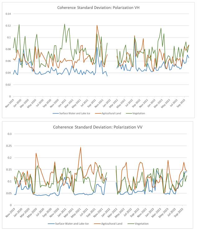
2.3.3. InSAR Coherence Time-Series Analysis

Different land cover types have unique physical properties and therefore may also have different coherence characteristics. However, the physical properties of each land cover are also temporally dynamic, such as lake ice phenology, crop harvest cycle, and vegetation growth. Hence, samples of three different earth land cover types were collected by adopting visual interpretation from Planetscope satellite images. The coherence values of three land cover types, representing surface water, agricultural land, and vegetation, are investigated at different times of year. Then, time-series analysis is performed by taking the mean and standard deviation of three cover types across different seasonal periods.
After the time-series analysis of coherence in the PPR region, three configurations of radar acquisitions are produced: the 2-band (backscatter values only for VV and VH), 4-band (backscatter, coherence for both VV and VH), and 6-band (backscatter, 12-day coherence, and 24-day coherence for VV and VH), shown in Table 1. These band configurations were used in this study for quantifying the accuracy improvement of using SAR coherence.

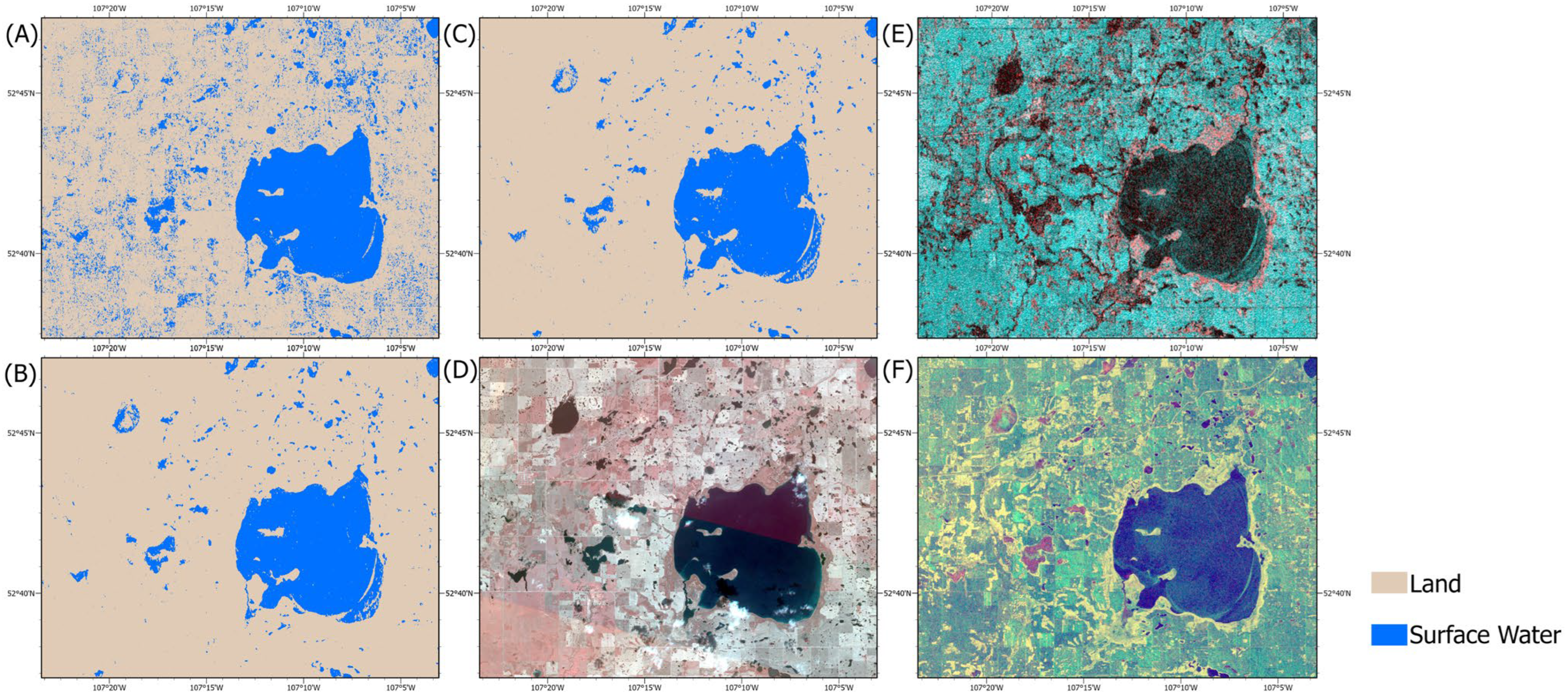
2.3.4. Image Classification and Post-Processing

Training and validation samples are randomly selected from permanent water pixels and permanent land pixels from the SWB product and are fitted into the random forest model for supervised learning. We extracted 80% of samples for training and 20% of samples for validation. The model is based on a set of independent decision trees, which uses ensemble learning and bootstrapping algorithms to reduce overfit in classification [74]. The performance of the random forest algorithm is dependent on three user-defined parameters: the number of decision trees in the model (number of trees), the number of features selected during each split (variables per split), and the minimum samples for each leaf node (min leaf population) [75]. Determining three hyperparameters can optimize the random forest model’s accuracy and efficiency by reducing its overfitting; 10-fold cross-validation will be applied to the parameter variables per split and min leaf population to determine a combination of two parameters with minimized generalization error [76]. Considering the time cost of tuning the parameters and the possible local minimum training loss, the Bayesian Hyperparameter Optimization was used for hyperparameter tuning [77]. The parameter number of trees is optimized under converged accuracy.
The post-processing of the morphological operators of opening and closing are applied to the classified image. Opening operators can be applied to remove micro-scaled water pixels on land, which are mainly sourced from speckle noise residuals. Closing operators can be applied to remove pixels classified as land in water bodies influenced by the increased surface roughness on water and the speckle effects of coherence on the surface water area. The final output is a 10 m resolution binary image product, representing the spatial distribution of surface water and land.

2.3.5. Accuracy Assessment

High-resolution optical imagery from the PlanetScope satellite is used to generate datasets for validation samples. Sample pixels are randomly collected from the optical image, and visual interpretation is conducted to label each sample. Collected samples are used to validate classified SAR images at different band configurations by constructing confusion matrices. Land pixels are considered negative, and water pixels are considered positive.

3. Results

The average coherence values for 12-day baseline coherence across three distinct land cover classes are provided in Figure 3 and Appendix B, as delineated by polarizations VH and VV. It is important to acknowledge a notable temporal data gap in Sentinel-1 observations over the study area from January 2022 to February 2022, precipitated by the cessation of Sentinel-1B mission operations due to equipment failure. In the context of surface water, coherence remains consistently low, hovering around 0.2 to 0.3 for polarization VV when snow and ice are not present. However, coherence exhibits a marked increase during the winter months spanning from December to April, with an average coherence surpassing 0.3 and peaking at 0.45 between January 2023 and March 2023. Conversely, the coherence levels for surface water using polarization VH linger around 0.2 to 0.25, with a less pronounced increase during winter months. Table 2 further underscores the pattern, revealing a general uptick in coherence across all land cover types during the winter period of December, January, and February compared to the summer months from June to August during the years 2020 and 2021.
In terms of the coherence averages across agricultural land and vegetation, a notable resemblance is observed in the seasonal coherence patterns of both land covers under polarization VV. Agricultural land consistently exhibits relatively higher coherence compared to vegetation. Both land cover types exhibit an increase in the pattern of coherence starting from October, peaking during the winter months around November and February, with agricultural land achieving an average coherence of 0.7, while vegetation hovers around 0.5 to 0.6. Throughout spring and summer, the coherence levels dip as vegetation and crops undergo growth phases. Interestingly, under polarization VV, coherence for both agricultural land and vegetation experiences significant drops in late October, early November, March, and April during the onset of freeze and melt when snowfall/snowmelt occurs. Conversely, polarization VH reveals a different trend, with vegetation showcasing higher coherence compared to agricultural land. Coherence peaks during the winter months, reaching values of 0.35, before declining to 0.25 in spring and being maintained around 0.3 during summer until the subsequent winter period (Table 2). In contrast, VH coherence on agricultural land follows a similar seasonal fluctuation pattern as vegetation, yet the coherence increase during winter is less pronounced. Additionally, the average coherence values for both agricultural land and vegetation remain relatively high during late spring compared to summer, following a notable decrease in coherence during March and April.
Temporal periods that exhibit high standard deviation might not be suitable for surface water extraction, since it has been demonstrated that different surface types may introduce uncertainty into the classification. Hence, the metric of standard deviation for three land cover types is essential for time-series analysis to investigate the separability of surface water and other land features, which is presented in Appendix C. The standard deviation of VV coherence for surface water is higher between December and March compared to other months, where the coherence standard deviation exceeds 0.1 in January 2020 and 2021, as well as in the winter period of 2022 and 2023. For agricultural land and vegetation, the highest standard deviation of coherence occurs mainly in May and October, varying from 0.15 to 0.2. For VH, the highest standard deviation of coherence is observed in vegetation during the winter and March of 2023, where the standard deviation reaches 0.12. Also, there is an increase in the standard deviation for all land cover types during September 2021 and July 2022.
The coherence of surface water using a 24-day temporal baseline at VH polarization is similar to coherence using a 12-day temporal baseline, with values approximating between 0.2 and 0.25. The mean VH coherence of vegetation and agricultural land is similar in that it ranges between 0.25 and 0.3. For VV, the increase in surface water coherence during winter is less prominent compared to the 12-day temporal baseline, with coherence being maintained around 0.3. Comparing the average VV coherence of the two temporal baselines, coherence for agricultural land and vegetation decreases more during late December and early January in the 24-day baseline than the 12-day. Appendix B illustrate the coherence average using 24-day temporal baselines.
For VH, the standard deviation of coherence using a 24-day temporal baseline is presented in Appendix B. There is no observed difference when compared to the 12-day temporal baseline in agricultural land and surface water except for vegetation, where the standard deviation of vegetation using a 24-day temporal baseline is less than the 12-day. For VV, the standard deviation of surface water for the 24-day baseline is lower than the 12-day baseline (Appendix C). Overall, there is no observable difference in the standard deviation of coherence for agricultural land when selecting different temporal baselines. For vegetation, the standard deviation of VV coherence decreases when choosing a 24-day baseline instead of a 12-day temporal baseline.
Figure 4, Figure 5 and Figure 6 present the contribution of InSAR coherence for surface water extraction for different seasonal periods. On 3 November 2019, the use of InSAR coherence improved the accuracy of surface water mapping, where most land cover types have higher coherence compared to surface water (Figure 4E). Figure 4 shows that at the Southwest of Redberry lake, large areas of Prairie grassland are classified as water, which demonstrates a higher amount of false positive errors. Also, some agricultural areas have been misclassified as surface water in the Southeast and North of Redberry lake. In addition, the backscatter imagery also indicates that the intensity of surface water and grassland is similar (Figure 4F). The overestimation of surface water can be reduced by using InSAR coherence for image features, which is demonstrated in four-band and six-band configuration (Figure 4B,C). By comparing the surface water extraction of using four-band configuration and six-band configuration, using the six-band configuration further reduces the overestimation of surface water due to the misclassification of Prairie grassland, but it also increases the omission error where more misclassification was observed due to image speckles in surface water (Figure 4B,C).
On 13 December 2019, the majority of waterbodies were frozen, which led to the increase in backscatter for surface water. In addition, the backscatter on land decreased during the winter period since the agricultural area was barren. As a result, Figure 5A shows that a large amount of misclassification from land to surface water occurred while using the intensity information only. The use of InSAR coherence effectively reduces the overestimation of surface water, but some omissions of surface water extraction were produced in the Redberry lake (Figure 4 and Figure 5). Pixels in these omission errors have higher coherence, whereas some pixels also have higher backscatter.
By observing intensity imagery at two seasonal periods within Redburry lake, the backscatter at some regions is higher, which leads to the variation in backscatter values in surface water (Figure 4F and Figure 5F). On the other hand, the coherence value at two seasonal periods illustrates that the coherence value in Redburry lake is spatially consistent (Figure 4E and Figure 5E). The increase in backscatter on waterbodies may be caused by local winds causing waves on water surface, producing Bragg scatter.
For the summer season of 29 August 2020, the contribution using InSAR coherence for surface water extraction is less significant compared to 3 November 2019. Although there is still some overestimation of surface water at Prairie grassland for two-band configuration, there is no difference in classification accuracy for band configuration using backscatter information only or band configuration that adds InSAR coherence as image features. The image composite of InSAR coherence illustrates that during the summer season, the coherence value of most agricultural and vegetation covers is decreased but that the backscatter is increased in these areas (Figure 6E,F).
Before applying the random forest classification to SAR imagery, five-fold cross-validation was used to optimize the model’s hyperparameters. This study focuses on optimizing the parameters “Variables per split” and “Min leaf population”, where optimized parameters and accuracies are presented in Table 3. It is worth mentioning that current training and testing accuracy is only used to determine the optimal parameters for random forest training, which will not be used for accuracy assessment.
To quantify the improvement in classification accuracy when using InSAR coherence, 750 validation samples from classified high-resolution optical satellite images were collected randomly at different seasonal periods from 2019 to 2020. Each validation sample was labeled using visual interpretation. Confusion matrices were generated based on validation samples for accuracy assessments. This study used confusion matrices of accuracy, F1-score, and Cohen’s Kappa score for accuracy assessments (Table 4).
During the summer and early autumn period, on 6 June 2020, 29 August 2020, and 4 October 2020, the extraction of surface water using only backscatter could achieve sufficient high accuracy, at 91.4%, 90.6%, and 84%, without using the post-processing algorithm, as well as achieving 94.5%, 93.9%, and 94.1% after using the post-processing algorithm. In this case, the contribution of InSAR coherence is not significant for surface water mapping and it might even decrease the accuracy. It has been shown that after using both 12-day and 24-day coherence instead of backscatter, the accuracy of surface water mapping after post-processing significantly decreased from 94.5% to 84.5% on 6 June 2020.
During the late autumn and winter period, on 3 November 2019, 13 December 2019, and 7 February 2020, the contribution of InSAR coherence to the accuracy of surface water extraction improved the classification results. The surface water mapping accuracy on 3 November 2019 using only backscatter was 83.7% without post-processing and 84% after post-classification, but it increased to 90.8% before post-processing and 92.9% with post-processing for four-band configuration. For the six-band configuration using both 12-day and 24-day coherence, the accuracy reached 91.6% before post-processing and 93.9% after post-processing. The accuracy on 21 December 2019, and 7 February 2020 using coherence also improved, ranging from 4% to 10%, where the improvement was more pronounced after applying the post-processing algorithm.
It is worth noting that between 19 April 2020, and 9 November 2020, the accuracy of surface water mapping was lower compared to other seasonal periods. The classification accuracy ranges from 82% to 84% for all three band configurations on 19 April 2020 before and after post-processing. On 9 November 2020, the accuracy lowered to below 80%; however, the accuracy using only backscatter was 72.2%, but increased to 77.9% using 12-day coherence data and 79% when using both 12-day and 24-day coherence features. Furthermore, 88% of classified images showed improvements when using four-band or with six-band configurations, with 44% exhibiting improvements to classification accuracy of greater than 5%.

4. Discussion

Based on the coherence time-series analysis results, InSAR coherence emerges as a potent feature for effectively distinguishing surface water from other land covers. Throughout the non-frozen season, surface water consistently exhibits low coherence. This phenomenon can be ascribed to two primary factors: firstly, the diminishing temporal correlation of phases, owing to the SAR backscatter signals being progressively deflected away from the sensor; and secondly, the coherence reduction, due to the variations in surface water roughness induced by wind and precipitation [32,37]. Despite the potential of increased backscatter caused by wind, coherence values decrease during windy periods, which compensates for the misclassification of surface water extraction using intensity features due to weather impact. During the winter period, the coherence average and standard deviation of surface water increase due to the formation of lake ice. It is shown that the coherence of some waterbodies will increase under certain ice formation conditions. In addition to the increase in coherence due to ice frozen to the bottom of waterbodies, as mentioned in other studies, ice cracking may also lead to higher coherence, which is illustrated in Figure 5 [39]. Hence, ice cracks and ice frozen to the bottom will result in higher coherence, which still leads to misclassification from surface water to land; this is still a challenge for surface water extraction [25]. Previous studies have indicated that ice frozen to the lake bed will lead to an increase in InSAR coherence since the backscatter interface was maintained at the lakebed at two SAR acquisitions. The considerable increase in coherence from bedfast lake ice is attributed to the signal interacting with the lake bottom and the removal of the ice–water interface that was previously dynamically changing position during ice growth [25].
The coherence on agricultural land varies due to seasonal impacts and the crop cycle. The coherence of VV polarization is relatively higher between the harvesting period to the agriculture growth period; this is expected due to crop structures not existing on agricultural landcover, which can be interpreted as barren land. The physical scattering characteristic of barren lands can be considered to be unchanged during the time interval of 12 or 24 days, which leads to a higher coherence. Apart from that, the decrease in coherence observed for agricultural land during late autumn and early spring imputes a change in the scattering source, which may be attributed to changes in soil moisture in these areas due to snow melting, which leads to a correlation decrease due to the difference in the relative permittivity between SAR acquisitions. Also, snowfall incidents caused a decrease in coherence during late autumn since the presence of the snow cover changes the backscatter characteristic of land covers. A main reason for the coherence loss of snow-covered terrain is a change in the liquid water content in the snow volume due to positive temperatures, melting, or rain [78]. On the other hand, the coherence is high for repeat-pass acquisitions for snow-covered land regions, which can be attributed to the sustained sub-freezing temperature at the study area keeping the snow volume dry and transmissive [62]. Coherence loss has been observed when there are snowpacks greater than 1 m in depth, which is why we do not expect to see considerable changes in coherence across the study area in the winter caused by snowfall or drifts.
During the summer and early autumn seasons between June and September, the coherence on agricultural land is maintained low, which explains the decrease in temporal correlation from the crop-growing period to the crop-harvesting period. Two factors might explain the low coherence during the crop growing period: the increase in crop heights can lead to changes in physical backscatter interactions, and the moisture of soil can result in changes in dielectric backscatter properties, consistent with crop classification using coherence in other regions [29,79].
Overall, the VH coherence provided better delineation relative to VV polarization for the discrimination of vegetation and surface water, but also exhibited a seasonal dependence. In general, VH coherence increases during the winter period for vegetated areas, which might be attributed to the sparse structure of vegetation canopies. During other seasonal periods, it might be difficult to separate surface water and vegetation using InSAR coherence since the scattering mechanism of the two land cover types is both easily affected by winds. However, it is sufficient to discriminate the surface water and vegetation using backscatter information only since the volume scattering effect of vegetation will result in a higher backscatter return.
By comparing the surface water extraction results of different temporal periods using confusion matrices, the contribution of InSAR coherence provides additional improvements to the overall classification during the autumn and winter periods compared to the spring and summer periods. During the spring and summer months, the emergence of grasses and the development of the canopy structure result in backscatter increases and coherence decreases, leading to diminished improvements when including coherence for surface water mapping. Apart from the comparison of classification results at different temporal periods, it is shown that using the post-processing algorithm will slightly increase the accuracy of surface water mapping.
During the time-series analysis of this study, this study examined the seasonal changes in coherence in surface water, agriculture, and vegetation. However, the seasonal changes in coherence on Prairie grassland were not investigated in this study. It might be beneficial to examine the seasonal changes in coherence and backscatter for Prairie grassland with different grass types and moisture levels in future studies. Although the InSAR coherence on Prairie grassland was not investigated, it is obvious that by combining backscatter and coherence data, misclassification from Prairie grassland to water can be reduced. The coherence of Prairie grassland was distinguishable from the coherence of surface water on 3 November 2019, 13 December 2019, and 29 August 2020, leading to the hypothesis that the backscatter and coherence of the Prairie grassland is complementary. Grass with taller heights increased the volume scattering effect, which increases the backscatter return, but the coherence might decrease since taller grass is more affected by the wind and the radar signals interact less with the land. It is worth mentioning that the salinity difference between Redburry lake and the surrounding freshwater lakes might lead to variation in backscatter return based on the contrast in scattering mechanisms, but this dielectric difference will not affect the timing of coherence gain/loss. Additionally, this study found that the use of co-polarized (VV) coherence demonstrated stronger separability between ice cover and land compared to cross-polarized (VH) coherence; this further improves the potential contribution of VV coherence on surface water mapping since the co-polarization can be considered less sensitive to surface ice types [80].
The choice of the InSAR temporal baseline affects coherence; it has a significant impact on coherence when the same satellite data with minimal vertical baseline are used. During this study, the selection of a 12-day temporal baseline or a 24-day temporal baseline during the winter period is investigated. This study attempted to use a longer temporal baseline in the winter to avoid the increased coherence of surface water due to ice frozen to the ground; however, the confusion matrices illustrated that there is no considerable difference for surface water mapping accuracy between using a longer temporal baseline and using a 12-day temporal baseline. Moreover, InSAR coherence using a smaller temporal baseline has not been fully investigated. Therefore, coherence analysis from other satellites with shorter revisit periods, such as the Radarsat Constellation Mission (RCM), or instantaneously from the Surface Water Ocean Topography (SWOT) mission can be explored in future studies [60]. Additionally, coherence analysis with a shorter revisit period will also provide more consistent and comprehensive information about seasonal changes and patterns of InSAR coherence in the PPR.

5. Conclusions

This study uses time-series analysis and confusion matrices to show that combining intensity information and coherence in SAR surface water extraction is effective during the seasonal period of fall and winter at the PPR, since the barren agricultural land and sparse grassland demonstrate higher coherence compared to water. The use of InSAR coherence effectively reduces the misclassification from land to water, but it might lead to omission errors from surface water extraction due to the speckle effect of the coherence product, surface water frozen to bottom, and ice surface deformations. After combining the InSAR coherence and backscatter, the improvement of classification accuracy can reach 10% during the winter period, but this improvement is less significant during the spring and summer period. It is shown that using VV polarization is more effective than VH polarization for discriminating between surface water and land. The study’s research and findings highlight how waterbodies and land can be efficiently distinguished by combining coherence as a classification feature. Additionally, InSAR coherence was observed to be most effective during the winter when changes in surface water dynamics are most muted, compared to the open water season where the location of target interaction changes due to wind and wave action. Limitations of this study were also discussed with several solutions being proposed for future studies, focusing specifically on SAR surface water mapping using coherence with different sensors and polarizations at other study areas.

Author Contributions

Conceptualization, P.C. and G.G.; methodology, P.C. and G.G.; validation, P.C. and G.G.; formal analysis, P.C.; investigation, P.C.; data curation, P.C.; writing—original draft preparation, P.C.; writing—review and editing, P.C. and G.G.; visualization, P.C.; supervision, G.G.; project administration, G.G.; All authors have read and agreed to the published version of the manuscript.

Funding

This research received no external funding and was conducted as a function of honors thesis preparation in support of undergraduate degree.

Institutional Review Board Statement

Not applicable.

Data Availability Statement

The data used in conducting this study are freely available through Google Earth Engine repository and the Copernicus Open Data Hub. Value-added coherence information is available upon request to the authors.

Conflicts of Interest

The authors declare no conflicts of interest.

Appendix A

Product NameAcquisition DatesSensorRel. Orbit
S1B_IW_SLC__1SDV_20191103T004906_20191103T004933_018756_0235A2_6ED6.SAFE20191103S1B5
S1B_IW_SLC__1SDV_20191115T004906_20191115T004933_018931_023B50_89EC.SAFE20191115S1B5
S1B_IW_SLC__1SDV_20191127T004906_20191127T004933_019106_0240EE_A42A.SAFE20191127S1B5
S1B_IW_SLC__1SDV_20191209T004905_20191209T004932_019281_024677_09EC.SAFE20191209S1B5
S1B_IW_SLC__1SDV_20191221T004905_20191221T004932_019456_024C0C_F4F1.SAFE20191221S1B5
S1B_IW_SLC__1SDV_20200102T004904_20200102T004931_019631_02519D_488D.SAFE20200102S1B5
S1B_IW_SLC__1SDV_20200114T004904_20200114T004931_019806_02572E_E304.SAFE20200114S1B5
S1B_IW_SLC__1SDV_20200126T004903_20200126T004930_019981_025CC4_35C9.SAFE20200126S1B5
S1B_IW_SLC__1SDV_20200207T004903_20200207T004930_020156_026277_488D.SAFE20200207S1B5
S1B_IW_SLC__1SDV_20200212T005705_20200212T005732_020229_0264E2_6B73.SAFE20200212S1B5
S1B_IW_SLC__1SDV_20200224T005704_20200224T005731_020404_026A83_43D4.SAFE20200224S1B5
S1B_IW_SLC__1SDV_20200302T004903_20200302T004930_020506_026DB7_679F.SAFE20200302S1B5
S1B_IW_SLC__1SDV_20200314T004903_20200314T004930_020681_027342_96CC.SAFE20200314S1B5
S1B_IW_SLC__1SDV_20200319T005705_20200319T005732_020754_0275A1_BFCC.SAFE20200319S1B5
S1B_IW_SLC__1SDV_20200331T005705_20200331T005732_020929_027B25_1C15.SAFE20200331S1B5
S1B_IW_SLC__1SDV_20200407T004903_20200407T004930_021031_027E52_440C.SAFE20200407S1B5
S1B_IW_SLC__1SDV_20200419T004904_20200419T004931_021206_0283DA_F5D6.SAFE20200419S1B5
S1B_IW_SLC__1SDV_20200501T004904_20200501T004931_021381_028961_7076.SAFE20200501S1B5
S1B_IW_SLC__1SDV_20200513T004905_20200513T004932_021556_028ED2_A5C4.SAFE20200513S1B5
S1B_IW_SLC__1SDV_20200525T004906_20200525T004933_021731_0293EF_7D08.SAFE20200525S1B5
S1B_IW_SLC__1SDV_20200606T004907_20200606T004933_021906_029930_9DEC.SAFE20200606S1B5
S1B_IW_SLC__1SDV_20200618T004907_20200618T004934_022081_029E79_A6C7.SAFE20200618S1B5
S1B_IW_SLC__1SDV_20200630T004908_20200630T004935_022256_02A3DA_A1A1.SAFE20200630S1B5
S1B_IW_SLC__1SDV_20200724T004909_20200724T004936_022606_02AE7A_0F1B.SAFE20200724S1B5
S1B_IW_SLC__1SDV_20200805T004910_20200805T004937_022781_02B3C8_D50B.SAFE20200805S1B5
S1B_IW_SLC__1SDV_20200817T004911_20200817T004938_022956_02B935_E8C4.SAFE20200817S1B5
S1B_IW_SLC__1SDV_20200829T004911_20200829T004938_023131_02BEB4_51BC.SAFE20200829S1B5
S1B_IW_SLC__1SDV_20200910T004912_20200910T004939_023306_02C433_B52A.SAFE20200910S1B5
S1B_IW_SLC__1SDV_20200922T004912_20200922T004939_023481_02C9AD_C801.SAFE20200922S1B5
S1B_IW_SLC__1SDV_20201004T004912_20201004T004939_023656_02CF28_9F43.SAFE20201004S1B5
S1B_IW_SLC__1SDV_20201016T004913_20201016T004940_023831_02D495_5778.SAFE20201016S1B5
S1B_IW_SLC__1SDV_20201028T004913_20201028T004940_024006_02DA16_3E33.SAFE20201028S1B5
S1B_IW_SLC__1SDV_20201109T004912_20201109T004939_024181_02DF7D_7D62.SAFE20201109S1B5
S1B_IW_SLC__1SDV_20201121T004912_20201121T004939_024356_02E4FC_0A41.SAFE20201121S1B5
S1B_IW_SLC__1SDV_20201203T004912_20201203T004939_024531_02EA8A_AD39.SAFE20201203S1B5
S1B_IW_SLC__1SDV_20201215T004911_20201215T004938_024706_02F037_D4E3.SAFE20201215S1B5
S1B_IW_SLC__1SDV_20201227T004911_20201227T004938_024881_02F5E4_2EB9.SAFE20201227S1B5
S1B_IW_SLC__1SDV_20210108T004910_20210108T004937_025056_02FB7E_BB56.SAFE20210108S1B5
S1B_IW_SLC__1SDV_20210120T004910_20210120T004937_025231_030119_7063.SAFE20210120S1B5
S1B_IW_SLC__1SDV_20210201T004909_20210201T004936_025406_0306A9_2B56.SAFE20210201S1B5
S1B_IW_SLC__1SDV_20210213T004909_20210213T004936_025581_030C65_2FCF.SAFE20210213S1B5
S1B_IW_SLC__1SDV_20210225T004909_20210225T004936_025756_03121B_8DBF.SAFE20210225S1B5
S1B_IW_SLC__1SDV_20210309T004909_20210309T004936_025931_0317D6_9B28.SAFE20210309S1B5
S1B_IW_SLC__1SDV_20210321T004909_20210321T004936_026106_031D76_EAE5.SAFE20210321S1B5
S1B_IW_SLC__1SDV_20210402T004909_20210402T004936_026281_0322F9_3EE5.SAFE20210402S1B5
S1B_IW_SLC__1SDV_20210414T004909_20210414T004936_026456_03288F_F58F.SAFE20210414S1B5
S1B_IW_SLC__1SDV_20210426T004910_20210426T004937_026631_032E2D_2CF1.SAFE20210426S1B5
S1B_IW_SLC__1SDV_20210508T004911_20210508T004938_026806_0333C6_2386.SAFE20210508S1B5
S1B_IW_SLC__1SDV_20210520T004911_20210520T004938_026981_033934_5596.SAFE20210520S1B5
S1B_IW_SLC__1SDV_20210601T004912_20210601T004939_027156_033E67_1A87.SAFE20210601S1B5
S1B_IW_SLC__1SDV_20210613T004913_20210613T004940_027331_0343A9_683C.SAFE20210613S1B5
S1B_IW_SLC__1SDV_20210625T004913_20210625T004940_027506_034894_0283.SAFE20210625S1B5
S1B_IW_SLC__1SDV_20210707T004914_20210707T004941_027681_034DB8_9E49.SAFE20210707S1B5
S1B_IW_SLC__1SDV_20210719T004915_20210719T004942_027856_0352EC_C813.SAFE20210719S1B5
S1B_IW_SLC__1SDV_20210731T004916_20210731T004943_028031_035808_E950.SAFE20210731S1B5
S1B_IW_SLC__1SDV_20210812T004916_20210812T004943_028206_035D73_EFAC.SAFE20210812S1B5
S1B_IW_SLC__1SDV_20210824T004917_20210824T004944_028381_0362ED_6885.SAFE20210824S1B5
S1B_IW_SLC__1SDV_20210905T004917_20210905T004944_028556_036865_9E2D.SAFE20210905S1B5
S1B_IW_SLC__1SDV_20210917T004918_20210917T004945_028731_036DC2_8DAE.SAFE20210917S1B5
S1B_IW_SLC__1SDV_20210929T004918_20210929T004945_028906_037321_6307.SAFE20210929S1B5
S1B_IW_SLC__1SDV_20211011T004918_20211011T004945_029081_03785E_AB3F.SAFE20211011S1B5
S1B_IW_SLC__1SDV_20211023T004919_20211023T004946_029256_037DCD_393F.SAFE20211023S1B5
S1B_IW_SLC__1SDV_20211104T004918_20211104T004945_029431_03832D_F81B.SAFE20211104S1B5
S1B_IW_SLC__1SDV_20211116T004918_20211116T004945_029606_038880_7681.SAFE20211116S1B5
S1B_IW_SLC__1SDV_20211128T004918_20211128T004945_029781_038DFC_0EBF.SAFE20211128S1B5
S1B_IW_SLC__1SDV_20211210T004917_20211210T004944_029956_039383_288B.SAFE20211210S1B5
S1B_IW_SLC__1SDV_20211222T004916_20211222T004943_030131_03990F_3583.SAFE20211222S1B5
S1A_IW_SLC__1SDV_20220227T132233_20220227T132303_042099_050403_D413.SAFE20220227S1B27
S1A_IW_SLC__1SDV_20220311T132233_20220311T132303_042274_0509F2_258F.SAFE20220311S1A27
S1A_IW_SLC__1SDV_20220323T132233_20220323T132303_042449_050FE8_68A5.SAFE20220323S1A27
S1A_IW_SLC__1SDV_20220404T132234_20220404T132303_042624_0515DD_9D99.SAFE20220404S1A27
S1A_IW_SLC__1SDV_20220416T132234_20220416T132304_042799_051BC0_316A.SAFE20220416S1A27
S1A_IW_SLC__1SDV_20220428T132234_20220428T132304_042974_052178_DC00.SAFE20220428S1A27
S1A_IW_SLC__1SDV_20220510T132235_20220510T132305_043149_052742_CF9D.SAFE20220510S1A27
S1A_IW_SLC__1SDV_20220522T132236_20220522T132306_043324_052C78_D2D4.SAFE20220522S1A27
S1A_IW_SLC__1SDV_20220603T132237_20220603T132307_043499_05319E_A6BB.SAFE20220603S1A27
S1A_IW_SLC__1SDV_20220615T132237_20220615T132307_043674_0536DC_1C04.SAFE20220615S1A27
S1A_IW_SLC__1SDV_20220627T132238_20220627T132308_043849_053C1A_45F7.SAFE20220627S1A27
S1A_IW_SLC__1SDV_20220709T132239_20220709T132309_044024_054148_A891.SAFE20220709S1A27
S1A_IW_SLC__1SDV_20220721T132240_20220721T132310_044199_054684_FAD7.SAFE20220721S1A27
S1A_IW_SLC__1SDV_20220802T132241_20220802T132310_044374_054BAE_AD35.SAFE20220802S1A27
S1A_IW_SLC__1SDV_20220814T132241_20220814T132311_044549_05512C_3ADE.SAFE20220814S1A27
S1A_IW_SLC__1SDV_20220826T132242_20220826T132312_044724_055712_555C.SAFE20220826S1A27
S1A_IW_SLC__1SDV_20220907T132243_20220907T132312_044899_055CF5_50E7.SAFE20220907S1A27
S1A_IW_SLC__1SDV_20220919T132242_20220919T132312_045074_0562DE_4152.SAFE20220919S1A27
S1A_IW_SLC__1SDV_20221001T132243_20221001T132313_045249_0568BA_3EFB.SAFE20221001S1A27
S1A_IW_SLC__1SDV_20221013T132243_20221013T132313_045424_056E98_64D7.SAFE20221013S1A27
S1A_IW_SLC__1SDV_20221025T132243_20221025T132313_045599_0573CA_A181.SAFE20221025S1A27
S1A_IW_SLC__1SDV_20221106T132243_20221106T132313_045774_0579B5_8581.SAFE20221106S1A27
S1A_IW_SLC__1SDV_20221118T132243_20221118T132312_045949_057F9A_3C64.SAFE20221118S1A27
S1A_IW_SLC__1SDV_20221130T132242_20221130T132312_046124_05858D_32A2.SAFE20221130S1A27
S1A_IW_SLC__1SDV_20221212T132242_20221212T132311_046299_058B83_85D6.SAFE20221212S1A27
S1A_IW_SLC__1SDV_20221224T132241_20221224T132311_046474_05917F_0FDC.SAFE20221224S1A27
S1A_IW_SLC__1SDV_20230105T132240_20230105T132310_046649_059767_7891.SAFE20230105S1A27
S1A_IW_SLC__1SDV_20230117T132239_20230117T132309_046824_059D51_F85D.SAFE20230117S1A27
S1A_IW_SLC__1SDV_20230129T132240_20230129T132309_046999_05A339_CEFF.SAFE20230129S1A27
S1A_IW_SLC__1SDV_20230210T132239_20230210T132309_047174_05A907_A125.SAFE20230210S1A27
S1A_IW_SLC__1SDV_20230222T132238_20230222T132308_047349_05AF01_5E17.SAFE20230222S1A27
S1A_IW_SLC__1SDV_20230306T132239_20230306T132309_047524_05B4EB_49C1.SAFE20230306S1A27
S1A_IW_SLC__1SDV_20230318T132239_20230318T132309_047699_05BAD9_F35F.SAFE20230318S1A27
S1A_IW_SLC__1SDV_20230330T132239_20230330T132309_047874_05C0B0_9BAF.SAFE20230330S1A27
S1A_IW_SLC__1SDV_20230411T132240_20230411T132309_048049_05C6A6_DE77.SAFE20230411S1A27
S1A_IW_SLC__1SDV_20230423T132240_20230423T132310_048224_05CC7C_C032.SAFE20230423S1A27
S1A_IW_SLC__1SDV_20230505T132240_20230505T132310_048399_05D25A_804B.SAFE20230505S1A27
S1A_IW_SLC__1SDV_20230517T132241_20230517T132311_048574_05D7AC_BA23.SAFE20230517S1A27
S1A_IW_SLC__1SDV_20230529T132242_20230529T132312_048749_05DCDF_49CB.SAFE20230529S1A27
S1A_IW_SLC__1SDV_20230610T132242_20230610T132312_048924_05E22A_B72C.SAFE20230610S1A27
S1A_IW_SLC__1SDV_20230622T132243_20230622T132312_049099_05E779_C5F7.SAFE20230622S1A27
S1A_IW_SLC__1SDV_20230704T132244_20230704T132313_049274_05ECD6_56E8.SAFE20230704S1A27
S1A_IW_SLC__1SDV_20230716T132245_20230716T132314_049449_05F241_A8AE.SAFE20230716S1A27
S1A_IW_SLC__1SDV_20230728T132245_20230728T132315_049624_05F7A0_B937.SAFE20230728S1A27
S1A_IW_SLC__1SDV_20230809T132245_20230809T132315_049799_05FD2C_B644.SAFE20230809S1A27
S1A_IW_SLC__1SDV_20230821T132246_20230821T132316_049974_060327_0333.SAFE20230821S1A27
S1A_IW_SLC__1SDV_20230902T132247_20230902T132317_050149_06092B_1DDE.SAFE20230902S1A27
S1A_IW_SLC__1SDV_20230914T132248_20230914T132317_050324_060F16_A738.SAFE20230914S1A27
S1A_IW_SLC__1SDV_20230926T132248_20230926T132318_050499_061515_C3B1.SAFE20230926S1A27

Appendix B

Glacies 02 00006 i001
Average coherence values for 12-day baseline coherence across three distinct land cover classes, delineated by polarization VH.

Appendix C

Glacies 02 00006 i002
Standard deviation of coherence for the three land cover types to highlight the separability of surface water compared to land features, shown in VH (top) and VV (bottom).

References

  1. Pekel, J.-F.; Cottam, A.; Gorelick, N.; Belward, A.S. High-Resolution Mapping of Global Surface Water and Its Long-Term Changes. Nature 2016, 540, 418–422. [Google Scholar] [CrossRef]
  2. Wang, S.; Li, J.; Russell, H.A.J. Methods for Estimating Surface Water Storage Changes and Their Evaluations. J. Hydrometeorol. 2023, 24, 445–461. [Google Scholar] [CrossRef]
  3. Olthof, I.; Rainville, T. Dynamic Surface Water Maps of Canada from 1984 to 2019 Landsat Satellite Imagery. Remote Sens. Environ. 2022, 279, 113121. [Google Scholar] [CrossRef]
  4. Wang, S.; Li, J. Terrestrial Water Storage Climatology for Canada from GRACE Satellite Observations in 2002–2014. Can. J. Remote Sens. 2016, 42, 190–202. [Google Scholar] [CrossRef]
  5. Li, J.; Wang, S.; Zhou, F. Time Series Analysis of Long-Term Terrestrial Water Storage over Canada from GRACE Satellites Using Principal Component Analysis. Can. J. Remote Sens. 2016, 42, 161–170. [Google Scholar] [CrossRef]
  6. Wang, S.; Yang, Y.; Luo, Y.; Rivera, A. Spatial and Seasonal Variations in Evapotranspiration over Canada’s Landmass. Hydrol. Earth Syst. Sci. 2013, 17, 3561–3575. [Google Scholar] [CrossRef]
  7. Fernandes, R.; Korolevych, V.; Wang, S. Trends in Land Evapotranspiration over Canada for the Period 1960–2000 Based on In Situ Climate Observations and a Land Surface Model. J. Hydrometeorol. 2007, 8, 1016–1030. [Google Scholar] [CrossRef]
  8. Chen, Y.; Wang, S.; Ren, Z.; Huang, J.; Wang, X.; Liu, S.; Deng, H.; Lin, W. Increased Evapotranspiration from Land Cover Changes Intensified Water Crisis in an Arid River Basin in Northwest China. J. Hydrol. 2019, 574, 383–397. [Google Scholar] [CrossRef]
  9. Li, J.; Wang, S.; Michel, C.; Russell, H.A.J. Surface Deformation Observed by InSAR Shows Connections with Water Storage Change in Southern Ontario. J. Hydrol. Reg. Stud. 2020, 27, 100661. [Google Scholar] [CrossRef]
  10. Li, W.; Zhang, W.; Li, Z.; Wang, Y.; Chen, H.; Gao, H.; Zhou, Z.; Hao, J.; Li, C.; Wu, X. A New Method for Surface Water Extraction Using Multi-Temporal Landsat 8 Images Based on Maximum Entropy Model. Eur. J. Remote Sens. 2022, 55, 303–312. [Google Scholar] [CrossRef]
  11. DeVries, B.; Huang, C.; Armston, J.; Huang, W.; Jones, J.W.; Lang, M.W. Rapid and Robust Monitoring of Flood Events Using Sentinel-1 and Landsat Data on the Google Earth Engine. Remote Sens. Environ. 2020, 240, 111664. [Google Scholar] [CrossRef]
  12. Pietroniro, A.; Leconte, R. A Review of Canadian Remote Sensing and Hydrology, 1999–2003. Hydrol. Process 2005, 19, 285–301. [Google Scholar] [CrossRef]
  13. Yang, X.; Zhao, S.; Qin, X.; Zhao, N.; Liang, L. Mapping of Urban Surface Water Bodies from Sentinel-2 MSI Imagery at 10 m Resolution via NDWI-Based Image Sharpening. Remote Sens. 2017, 9, 596. [Google Scholar] [CrossRef]
  14. Wang, C.; Jia, M.; Chen, N.; Wang, W. Long-Term Surface Water Dynamics Analysis Based on Landsat Imagery and the Google Earth Engine Platform: A Case Study in the Middle Yangtze River Basin. Remote Sens. 2018, 10, 1635. [Google Scholar] [CrossRef]
  15. Mustafa, M.T.; Hassoon, K.I.; Hussain, H.M.; Abd, M.H. Using water indices (NDWI, MNDWI, NDMI, WRI and AWEI) to detect physical and chemical parameters by apply remote sensing and GIS techniques. Int. J. Res.-Granthaalayah 2017, 5, 117–128. [Google Scholar] [CrossRef]
  16. McFEETERS, S.K. The Use of the Normalized Difference Water Index (NDWI) in the Delineation of Open Water Features. Int. J. Remote Sens. 1996, 17, 1425–1432. [Google Scholar] [CrossRef]
  17. Xu, H. Modification of Normalised Difference Water Index (NDWI) to Enhance Open Water Features in Remotely Sensed Imagery. Int. J. Remote Sens. 2006, 27, 3025–3033. [Google Scholar] [CrossRef]
  18. Kasischke, E.S.; Melack, J.M.; Craig Dobson, M. The Use of Imaging Radars for Ecological Applications—A Review. Remote Sens. Environ. 1997, 59, 141–156. [Google Scholar] [CrossRef]
  19. Li, J.; Wang, S. An Automatic Method for Mapping Inland Surface Waterbodies with Radarsat-2 Imagery. Int. J. Remote Sens. 2015, 36, 1367–1384. [Google Scholar] [CrossRef]
  20. Brisco, B. Mapping and Monitoring Surface Water and Wetlands with Synthetic Aperture Radar. In Remote Sensing of Wetlands: Applications and Advances; CRC Press: Boca Raton, FL, USA, 2015; pp. 119–136. [Google Scholar]
  21. Martinis, S.; Twele, A.; Voigt, S. Towards Operational near Real-Time Flood Detection Using a Split-Based Automatic Thresholding Procedure on High Resolution TerraSAR-X Data. Nat. Hazards Earth Syst. Sci. 2009, 9, 303–314. [Google Scholar] [CrossRef]
  22. White, L.; Brisco, B.; Pregitzer, M.; Tedford, B.; Boychuk, L. RADARSAT-2 Beam Mode Selection for Surface Water and Flooded Vegetation Mapping. Can. J. Remote Sens. 2014, 40, 135–151. [Google Scholar]
  23. Millard, K.; Brown, N.; Stiff, D.; Pietroniro, A. Automated Surface Water Detection from Space: A Canada-Wide, Open-Source, Automated, near-Real Time Solution. Can. Water Resour. J./Rev. Can. Des Ressour. Hydr. 2020, 45, 304–323. [Google Scholar] [CrossRef]
  24. Morris, K.; Jeffries, M.O.; Weeks, W.F. Ice Processes and Growth History on Arctic and Sub-Arctic Lakes Using ERS-1 SAR Data. Polar Rec. 1995, 31, 115–128. [Google Scholar] [CrossRef]
  25. Murfitt, J.; Duguay, C.R. Assessing the Performance of Methods for Monitoring Ice Phenology of the World’s Largest High Arctic Lake Using High-Density Time Series Analysis of Sentinel-1 Data. Remote Sens. 2020, 12, 382. [Google Scholar] [CrossRef]
  26. Martinis, S.; Plank, S.; Ćwik, K. The Use of Sentinel-1 Time-Series Data to Improve Flood Monitoring in Arid Areas. Remote Sens. 2018, 10, 583. [Google Scholar] [CrossRef]
  27. Huang, W.; DeVries, B.; Huang, C.; Lang, M.W.; Jones, J.W.; Creed, I.F.; Carroll, M.L. Automated Extraction of Surface Water Extent from Sentinel-1 Data. Remote Sens. 2018, 10, 797. [Google Scholar] [CrossRef]
  28. Bartsch, A.; Trofaier, A.M.; Hayman, G.; Sabel, D.; Schlaffer, S.; Clark, D.B.; Blyth, E. Detection of Open Water Dynamics with ENVISAT ASAR in Support of Land Surface Modelling at High Latitudes. Biogeosciences 2012, 9, 703–714. [Google Scholar] [CrossRef]
  29. Nasirzadehdizaji, R.; Cakir, Z.; Balik Sanli, F.; Abdikan, S.; Pepe, A.; Calò, F. Sentinel-1 Interferometric Coherence and Backscattering Analysis for Crop Monitoring. Comput. Electron. Agric. 2021, 185, 106118. [Google Scholar] [CrossRef]
  30. Schlaffer, S.; Chini, M.; Dorigo, W.; Plank, S. Monitoring Surface Water Dynamics in the Prairie Pothole Region of North Dakota Using Dual-Polarised Sentinel-1 Synthetic Aperture Radar (SAR) Time Series. Hydrol. Earth Syst. Sci. 2022, 26, 841–860. [Google Scholar] [CrossRef]
  31. Canisius, F.; Brisco, B.; Murnaghan, K.; Van Der Kooij, M.; Keizer, E. SAR Backscatter and InSAR Coherence for Monitoring Wetland Extent, Flood Pulse and Vegetation: A Study of the Amazon Lowland. Remote Sens. 2019, 11, 720. [Google Scholar] [CrossRef]
  32. Amani, M.; Poncos, V.; Brisco, B.; Foroughnia, F.; DeLancey, E.R.; Ranjbar, S. InSAR Coherence Analysis for Wetlands in Alberta, Canada Using Time-Series Sentinel-1 Data. Remote Sens. 2021, 13, 3315. [Google Scholar] [CrossRef]
  33. Touzi, R.; Lopes, A.; Bruniquel, J.; Vachon, P.W. Coherence Estimation for SAR Imagery. IEEE Trans. Geosci. Remote Sens. 1999, 37, 135–149. [Google Scholar] [CrossRef]
  34. Ullmann, T.; Sauerbrey, J.; Hoffmeister, D.; May, S.M.; Baumhauer, R.; Bubenzer, O. Assessing Spatiotemporal Variations of Sentinel-1 InSAR Coherence at Different Time Scales over the Atacama Desert (Chile) between 2015 and 2018. Remote Sens. 2019, 11, 2960. [Google Scholar] [CrossRef]
  35. Ni, J.; Lopez-Martinez, C.; Hu, Z.; Zhang, F. Multitemporal SAR and Polarimetric SAR Optimization and Classification: Reinterpreting Temporal Coherence. IEEE Trans. Geosci. Remote Sens. 2022, 60, 5236617. [Google Scholar] [CrossRef]
  36. Chul Jung, H.; Alsdorf, D. Repeat-Pass Multi-Temporal Interferometric SAR Coherence Variations with Amazon Floodplain and Lake Habitats. Int. J. Remote Sens. 2010, 31, 881–901. [Google Scholar] [CrossRef]
  37. Smith, L.C.; Alsdorf, D.E. Control on Sediment and Organic Carbon Delivery to the Arctic Ocean Revealed with Space-Borne Synthetic Aperture Radar: Ob’ River, Siberia. Geology 1998, 26, 395. [Google Scholar] [CrossRef]
  38. Lu, Z.; Kwoun, O. Radarsat-1 and ERS InSAR Analysis Over Southeastern Coastal Louisiana: Implications for Mapping Water-Level Changes Beneath Swamp Forests. IEEE Trans. Geosci. Remote Sens. 2008, 46, 2167–2184. [Google Scholar] [CrossRef]
  39. Antonova, S.; Duguay, C.R.; Kääb, A.; Heim, B.; Langer, M.; Westermann, S.; Boike, J. Monitoring Bedfast Ice and Ice Phenology in Lakes of the Lena River Delta Using TerraSAR-X Backscatter and Coherence Time Series. Remote Sens. 2016, 8, 903. [Google Scholar] [CrossRef]
  40. Pandit, A.; Sawant, S.; Mohite, J.; Pappula, S. Sentinel-1-Derived Coherence Time-Series for Crop Monitoring in Indian Agriculture Region. Geocarto Int. 2022, 37, 9497–9517. [Google Scholar] [CrossRef]
  41. De Vroey, M.; Radoux, J.; Defourny, P. Grassland Mowing Detection Using Sentinel-1 Time Series: Potential and Limitations. Remote Sens. 2021, 13, 348. [Google Scholar] [CrossRef]
  42. Tamm, T.; Zalite, K.; Voormansik, K.; Talgre, L. Relating Sentinel-1 Interferometric Coherence to Mowing Events on Grasslands. Remote Sens. 2016, 8, 802. [Google Scholar] [CrossRef]
  43. Li, Z.; Guo, H.; Li, X.; Wang, C. SAR Interferometry Coherence Analysis for Snow Mapping. In Scanning the Present and Resolving the Future, Proceedings of the IEEE 2001 International Geoscience and Remote Sensing Symposium, Sydney, NSW, Australia, 9–13 July 2001; IEEE: New York, NY, USA, 2001; Volume 6, pp. 2905–2907. [Google Scholar] [CrossRef]
  44. Kumar, V.; Venkataraman, G. SAR interferometric coherence analysis for snow cover mapping in the Western Himalayan region. Int. J. Digit. Earth 2011, 4, 78–90. [Google Scholar] [CrossRef]
  45. Yu, Z.; An, Q.; Liu, W.; Wang, Y. Analysis and Evaluation of Surface Water Changes in the Lower Reaches of the Yangtze River Using Sentinel-1 Imagery. J. Hydrol. Reg. Stud. 2022, 41, 101074. [Google Scholar] [CrossRef]
  46. Zhang, M.; Chen, F.; Tian, B.; Liang, D. Multi-Temporal SAR Image Classification of Coastal Plain Wetlands Using a New Feature Selection Method and Random Forests. Remote Sens. Lett. 2019, 10, 312–321. [Google Scholar] [CrossRef]
  47. Zhou, Z.; Liu, L.; Jiang, L.; Feng, W.; Samsonov, S.V. Using Long-Term SAR Backscatter Data to Monitor Post-Fire Vegetation Recovery in Tundra Environment. Remote Sens. 2019, 11, 2230. [Google Scholar] [CrossRef]
  48. Bangira, T.; Alfieri, S.M.; Menenti, M.; Van Niekerk, A. Comparing Thresholding with Machine Learning Classifiers for Mapping Complex Water. Remote Sens. 2019, 11, 1351. [Google Scholar] [CrossRef]
  49. Yue, L.; Li, B.; Zhu, S.; Yuan, Q.; Shen, H. A Fully Automatic and High-Accuracy Surface Water Mapping Framework on Google Earth Engine Using Landsat Time-Series. Int. J. Digit. Earth 2023, 16, 210–233. [Google Scholar] [CrossRef]
  50. Maghsoudi, Y.; Collins, M.J.; Leckie, D.G. Radarsat-2 Polarimetric SAR Data for Boreal Forest Classification Using SVM and a Wrapper Feature Selector. IEEE J. Sel. Top. Appl. Earth Obs. Remote Sens. 2013, 6, 1531–1538. [Google Scholar] [CrossRef]
  51. Jacob, A.W.; Vicente-Guijalba, F.; Lopez-Martinez, C.; Lopez-Sanchez, J.M.; Litzinger, M.; Kristen, H.; Mestre-Quereda, A.; Ziolkowski, D.; Lavalle, M.; Notarnicola, C.; et al. Sentinel-1 InSAR Coherence for Land Cover Mapping: A Comparison of Multiple Feature-Based Classifiers. IEEE J. Sel. Top. Appl. Earth Obs. Remote Sens. 2020, 13, 535–552. [Google Scholar] [CrossRef]
  52. Zhang, X.; Chan, N.W.; Pan, B.; Ge, X.; Yang, H. Mapping Flood by the Object-Based Method Using Backscattering Coefficient and Interference Coherence of Sentinel-1 Time Series. Sci. Total Environ. 2021, 794, 148388. [Google Scholar] [CrossRef]
  53. Mestre-Quereda, A.; Lopez-Sanchez, J.M.; Vicente-Guijalba, F.; Jacob, A.W.; Engdahl, M.E. Time-Series of Sentinel-1 Interferometric Coherence and Backscatter for Crop-Type Mapping. IEEE J. Sel. Top. Appl. Earth Obs. Remote Sens. 2020, 13, 4070–4084. [Google Scholar] [CrossRef]
  54. Nikaein, T.; Iannini, L.; Molijn, R.A.; Lopez-Dekker, P. On the Value of Sentinel-1 InSAR Coherence Time-Series for Vegetation Classification. Remote Sens. 2021, 13, 3300. [Google Scholar] [CrossRef]
  55. Hansen, J.N.; Mitchard, E.T.A.; King, S. Assessing Forest/Non-Forest Separability Using Sentinel-1 C-Band Synthetic Aperture Radar. Remote Sens. 2020, 12, 1899. [Google Scholar] [CrossRef]
  56. Wu, Q.; Lane, C.R. Delineation and Quantification of Wetland Depressions in the Prairie Pothole Region of North Dakota. Wetlands 2016, 36, 215–227. [Google Scholar] [CrossRef]
  57. Winter, T.C. Hydrologic Studies of Wetlands in the Northern Prairie. In Northern Prairie Wetlands; Iowa State University Press: Ames, IA, USA, 1989. [Google Scholar]
  58. Cohen, M.J.; Creed, I.F.; Alexander, L.; Basu, N.B.; Calhoun, A.J.K.; Craft, C.; D’Amico, E.; DeKeyser, E.; Fowler, L.; Golden, H.E.; et al. Do Geographically Isolated Wetlands Influence Landscape Functions? Proc. Natl. Acad. Sci. USA 2016, 113, 1978–1986. [Google Scholar] [CrossRef]
  59. Montgomery, J.S.; Hopkinson, C.; Brisco, B.; Patterson, S.; Rood, S.B. Wetland Hydroperiod Classification in the Western Prairies Using Multitemporal Synthetic Aperture Radar. Hydrol. Process 2018, 32, 1476–1490. [Google Scholar] [CrossRef]
  60. Yagmur, N.; Bilgilioglu, B.B.; Dervisoglu, A.; Musaoglu, N.; Tanik, A. Long and short-term assessment of surface area changes in saline and freshwater lakes via remote sensing. Water Environ. J. 2020, 35, 107–122. [Google Scholar] [CrossRef]
  61. Weather Spark. Saskatoon Climate, Weather By Month, Average Temperature (Canada). Available online: http://weatherspark.com/y/3392/Average-Weather-in-Saskatoon-Canada-Year-Round (accessed on 23 January 2024).
  62. Government of Canada. Almanac Averages and Extremes for January 22. (October 2024). 2024. Available online: https://climate.weather.gc.ca/climate_data/almanac_e.html?hlyRange=2013-11-12%7C2025-01-22&dlyRange=2013-03-09%7C2025-01-22&mlyRange=%7C&StationID=51878&Prov=SK&urlExtension=_e.html&searchType=stnName&optLimit=yearRange&StartYear=1840&EndYear=2025&selRowPerPage=25&Line=2&searchMethod=contains&month=1&day=22&txtStationName=prince%2Balbert&timeframe=4&Year=2025&time=LST (accessed on 25 January 2025).
  63. Torres, R.; Snoeij, P.; Geudtner, D.; Bibby, D.; Davidson, M.; Attema, E.; Potin, P.; Rommen, B.; Floury, N.; Brown, M.; et al. GMES Sentinel-1 Mission. Remote Sens. Environ. 2012, 120, 9–24. [Google Scholar] [CrossRef]
  64. Gorelick, N.; Hancher, M.; Dixon, M.; Ilyushchenko, S.; Thau, D.; Moore, R. Google Earth Engine: Planetary-Scale Geospatial Analysis for Everyone. Remote Sens. Environ. 2017, 202, 18–27. [Google Scholar] [CrossRef]
  65. Gatelli, F.; Monti Guamieri, A.; Parizzi, F.; Pasquali, P.; Prati, C.; Rocca, F. The Wavenumber Shift in SAR Interferometry. IEEE Trans. Geosci. Remote Sens. 1994, 32, 855–865. [Google Scholar] [CrossRef]
  66. Wang, X.; Xiao, X.; Zou, Z.; Dong, J.; Qin, Y.; Doughty, R.B.; Menarguez, M.A.; Chen, B.; Wang, J.; Ye, H.; et al. Gainers and Losers of Surface and Terrestrial Water Resources in China during 1989–2016. Nat. Commun. 2020, 11, 3471. [Google Scholar] [CrossRef]
  67. Planet Labs Inc. Planet Imagery Product Specifications: PlanetScope & RapidEye; Planet Labs Inc.: San Francisco, CA, USA, 2019; Available online: https://assets.planet.com/docs/combined-imagery-product-spec-april-2019.pdf (accessed on 13 May 2025).
  68. Mullissa, A.; Vollrath, A.; Odongo-Braun, C.; Slagter, B.; Balling, J.; Gou, Y.; Gorelick, N.; Reiche, J. Sentinel-1 SAR Backscatter Analysis Ready Data Preparation in Google Earth Engine. Remote Sens. 2021, 13, 1954. [Google Scholar] [CrossRef]
  69. Lee, T.F. Sea Ice-Edge Enhancement Using Polar-Orbiting Environmental Satellite Data. Weather. Forecast. 1993, 8, 369–377. [Google Scholar] [CrossRef]
  70. Lee, J.-S. A Simple Speckle Smoothing Algorithm for Synthetic Aperture Radar Images. IEEE Trans. Syst. Man. Cybern. 1983, SMC-13, 85–89. [Google Scholar] [CrossRef]
  71. Vollrath, A.; Mullissa, A.; Reiche, J. Angular-Based Radiometric Slope Correction for Sentinel-1 on Google Earth Engine. Remote Sens. 2020, 12, 1867. [Google Scholar] [CrossRef]
  72. Yague-Martinez, N.; Prats-Iraola, P.; Rodriguez Gonzalez, F.; Brcic, R.; Shau, R.; Geudtner, D.; Eineder, M.; Bamler, R. Interferometric Processing of Sentinel-1 TOPS Data. IEEE Trans. Geosci. Remote Sens. 2016, 54, 2220–2234. [Google Scholar] [CrossRef]
  73. Prats-Iraola, P.; Scheiber, R.; Marotti, L.; Wollstadt, S.; Reigber, A. TOPS Interferometry With TerraSAR-X. IEEE Trans. Geosci. Remote Sens. 2012, 50, 3179–3188. [Google Scholar] [CrossRef]
  74. Breiman, L. Random Forests. Mach. Learn. 2001, 45, 5–32. [Google Scholar] [CrossRef]
  75. Belgiu, M.; Drăguţ, L. Random Forest in Remote Sensing: A Review of Applications and Future Directions. ISPRS J. Photogramm. Remote Sens. 2016, 114, 24–31. [Google Scholar] [CrossRef]
  76. Agarwal, V.; Akyilmaz, O.; Shum, C.K.; Feng, W.; Yang, T.Y.; Forootan, E.; Syed, T.H.; Haritashya, U.K.; Uz, M. Machine learning based downscaling of Grace-estimated groundwater in Central Valley, California. Sci. Total Environ. 2023, 865, 161138. [Google Scholar] [CrossRef]
  77. Agrawal, T. Bayesian optimization. In Hyperparameter Optimization in Machine Learning; Apress: Berkeley, CA, USA, 2020; pp. 81–108. [Google Scholar] [CrossRef]
  78. Leinss, S.; Wiesmann, A.; Lemmetyinen, J.; Hajnsek, I. Snow water equivalent of dry snow measured by differential interferometry. IEEE J. Sel. Top. Appl. Earth Obs. Remote Sens. 2015, 8, 3773–3790. [Google Scholar] [CrossRef]
  79. Villarroya-Carpio, A.; Lopez-Sanchez, J.M.; Engdahl, M.E. Sentinel-1 Interferometric Coherence as a Vegetation Index for Agriculture. Remote Sens. Environ. 2022, 280, 113208. [Google Scholar] [CrossRef]
  80. Gunn, G.E.; Duguay, C.R.; Derksen, C.; Clausi, D.A.; Toose, P. Investigating the influence of variable freshwater ice types on passive and active microwave observations. Remote Sens. 2017, 9, 1242. [Google Scholar] [CrossRef]
Figure 1. Study area for surface water extent extraction surrounding Redburry lake (52.692206–107.138532°) within the Pothole Prairie Region, located northwest of Saskatoon, Saskatchewan.
Glacies 02 00006 g001
Figure 2. Overall workflow diagram for Sentinel-1 surface water extraction using backscatter and coherence data.
Glacies 02 00006 g002
Figure 3. Time-series analysis of average VV coherence observed for surface water, agricultural land, and vegetation landcover types in the Prairie Pothole Region.
Glacies 02 00006 g003
Figure 4. Surface water classification result of three band configuration and image composite of the study area at 3 November 2019: (A) 2-band configuration; (B) 4-band configuration; (C) 6-band configuration; (D) planet scope imagery in NIR, green, and blue composites; (E) 12-day coherence imagery in composites of VH, VV, and VV; (F) backscatter imagery in composites of VH, VV, and VH/VV.
Glacies 02 00006 g004
Figure 5. Surface water classification result of three band configuration and image composite of the study area at 13 December 2019: (A) two-band configuration; (B) four-band configuration; (C) six-band configuration; (D) planet scope imagery in NIR, green, and blue composites; (E) 12-day coherence imagery in composites of VH, VV, and VV; (F) backscatter imagery in composites of VH, VV, and VH/VV.
Glacies 02 00006 g005
Figure 6. Surface water classification result of three band configuration and image composite of the study area at 29 August 2020: (A) two-band configuration; (B) four-band configuration; (C) six-band configuration; (D) planet scope imagery in NIR, green, and blue composites; (E) 12-day coherence imagery in composites of VH, VV, and VV; (F) backscatter imagery in composites of VH, VV, and VH/VV.
Glacies 02 00006 g006
Table 1. Band configurations that are compared in this study.
Band Used
2-BandBackscatter: VV, VH
4-BandBackscatter: VV, VH
Coherence (12-day): VV, VH
6-BandBackscatter: VV, VH
Coherence (12 days): VV, VH
Coherence (24 days): VV, VH
Table 2. Monthly coherence average using a 12-day temporal baseline for 2020–2021. The coherence during the winter season for each landcover type is higher relative to the summer season, particularly at VV polarization.
WinterSummer
PolarizationLand CoverDecember 2020January
2021
February
2021
January
2020
July
2020
August
2020
VHSurface Water0.220.220.230.220.220.22
Agriculture0.270.250.260.270.250.25
Vegetation0.340.330.300.260.260.28
VVSurface Water0.360.330.330.240.240.22
Agriculture0.690.580.570.370.260.32
Vegetation0.530.490.450.300.290.32
Table 3. Parameter optimization and accuracy at different band configurations and temporal periods. VarSplit = variables per spliat; MinLeaf = minimum leaf population; Train Acc = training accuracy; Test Acc = testing accuracy.
DateConfigurationVarSplitMinLeafTrain AccTest Acc
11/3/20192-band1200.9640.95
4-band320.9820.99
6-band110.9930.99
12/21/20192-band250.9450.94
4-band420.9830.97
6-band210.9810.968
2/7/20202-band250.9780.956
4-band420.9740.97
6-band250.9760.968
4/19/20202-band110.9740.97
4-band4100.9740.98
6-band250.9730.974
6/6/20202-band120.99430.99
4-band220.9940.99
6-band2100.9930.986
8/29/20202-band1100.9910.99
4-band410.9950.99
6-band350.9920.981
10/4/20202-band150.910.89
4-band150.9860.98
6-band220.9750.97
11/9/20202-band1100.8310.83
4-band2200.8520.86
6-band250.8520.85
Table 4. Confusion matrix of different band configurations at different temporal periods without post-processing algorithm. TP = true positive; FP = false positive; FN = false negative; Acc = overall accuracy; F1 = F1 score where values approaching 1 represent a high precision and recall. Italicized cells have the post-processing algorithm applied.
DateConfigurationTPFPFNTNAccF1Kappa
11/3/20192-band257292653156893723380.840.840.810.830.670.68
4-band266283574012134154140.910.930.890.910.810.85
6-band2622805841234284260.920.940.890.930.830.88
12/21/20192-band257284684047963783320.850.820.820.810.690.64
4-band2482707051424284270.900.930.870.910.790.85
6-band2412578166444244230.890.910.850.880.760.81
2/7/20202-band254283724054953703320.830.820.800.810.660.64
4-band252283664022394103880.880.890.850.880.760.79
6-band258276664827423993860.880.880.850.860.740.76
4/19/20202-band276305583570983403060.830.820.810.820.650.65
4-band272302683860853443190.830.840.810.830.650.67
6-band273306713850733503270.840.850.820.850.670.70
6/6/20202-band2763006340014054030.920.950.900.940.830.89
4-band2752996541114034030.910.940.890.930.820.89
6-band27430266382774023270.910.850.890.840.810.69
8/29/20202-band2602886537364144110.910.940.880.930.810.88
4-band2642856039134174150.920.940.900.930.830.88
6-band2742875340004154150.930.950.910.930.850.89
10/4/20202-band27028854356373584090.840.940.820.930.680.88
4-band26929955269134094040.910.950.890.940.820.89
6-band27030057277184083970.910.940.890.930.820.88
11/9/20202-band19525012772631293572910.740.730.670.710.470.46
4-band1912331369448703673450.750.780.680.740.480.55
6-band1982291259445583743610.770.790.700.750.510.57
Disclaimer/Publisher’s Note: The statements, opinions and data contained in all publications are solely those of the individual author(s) and contributor(s) and not of MDPI and/or the editor(s). MDPI and/or the editor(s) disclaim responsibility for any injury to people or property resulting from any ideas, methods, instructions or products referred to in the content.

