
Bootstrap Methods for Bias-Correcting Probability Distribution Parameters Characterizing Extreme Snow Accumulations


Abstract
1. Introduction
2. Literature Background
2.1. Bias Correction
2.2. Reliability-Targeted Loads
3. Methods
- Train/fit using available data.
- Obtain residuals , which are assumed to follow a normal distribution.
- Fit the true to a specified distribution and obtain the initial scale parameter of the distribution .
- Letting b represent one of B bootstrap samples, perform the following:
- Obtain new responses by bootstrapping the residuals and adding to the predicted responses:where represents a simulated alternative to based on a bootstrap sample of residual terms.
- Estimate the scale parameter of the specified distribution () and other related parameters (i.e., , ) for each boostrap set ().
- Find the percentile () of the estimates of that is closest to . The closest spread parameter is denoted as .
- Sort the boostrap estimates in ascending order.
- For each estimate (where ), calculate the absolute difference from :
- Find the estimate that has the smallest absolute difference from . Mathematically, this is equivalent to finding the index j such that . Then, , and is accompanied by its corresponding parameters (i.e., , ).
- Calculate the percentile position of within the sorted list of estimates. The percentile is given by the following formula:
- Predict using the regression-based model in the above algorithm.
- Letting b represent one of B bootstrap samples, perform the following:
- Fit to a specified distribution and obtain and other corresponding parameters (i.e., , ).
- Calculate the percentile position of sigma () within the sorted list of estimates. The percentile is given by the following formula:
- Given a specific statistic value from the above algorithm, find the in the bootstrap distribution that is associated with . Conceptually, this can be expressed as for the b where is minimized. The computed is accompanied by its corresponding parameters (i.e., , ).
4. Simulations
- , with for ;
- for and where ;
- and for ;
- for .
- for ;
- , , , , , and ;
- for .
4.1. Experimental Setup
- Selecting the best percentile () from the sampling distribution of the parameter that corrects for the bias in for the training data.
- Generating the sampling distribution of and using the test dataset with a bootstrap sample size of 200.
- Using , selecting the least biased parameter along with its parameter from the sampling distribution for the test data.
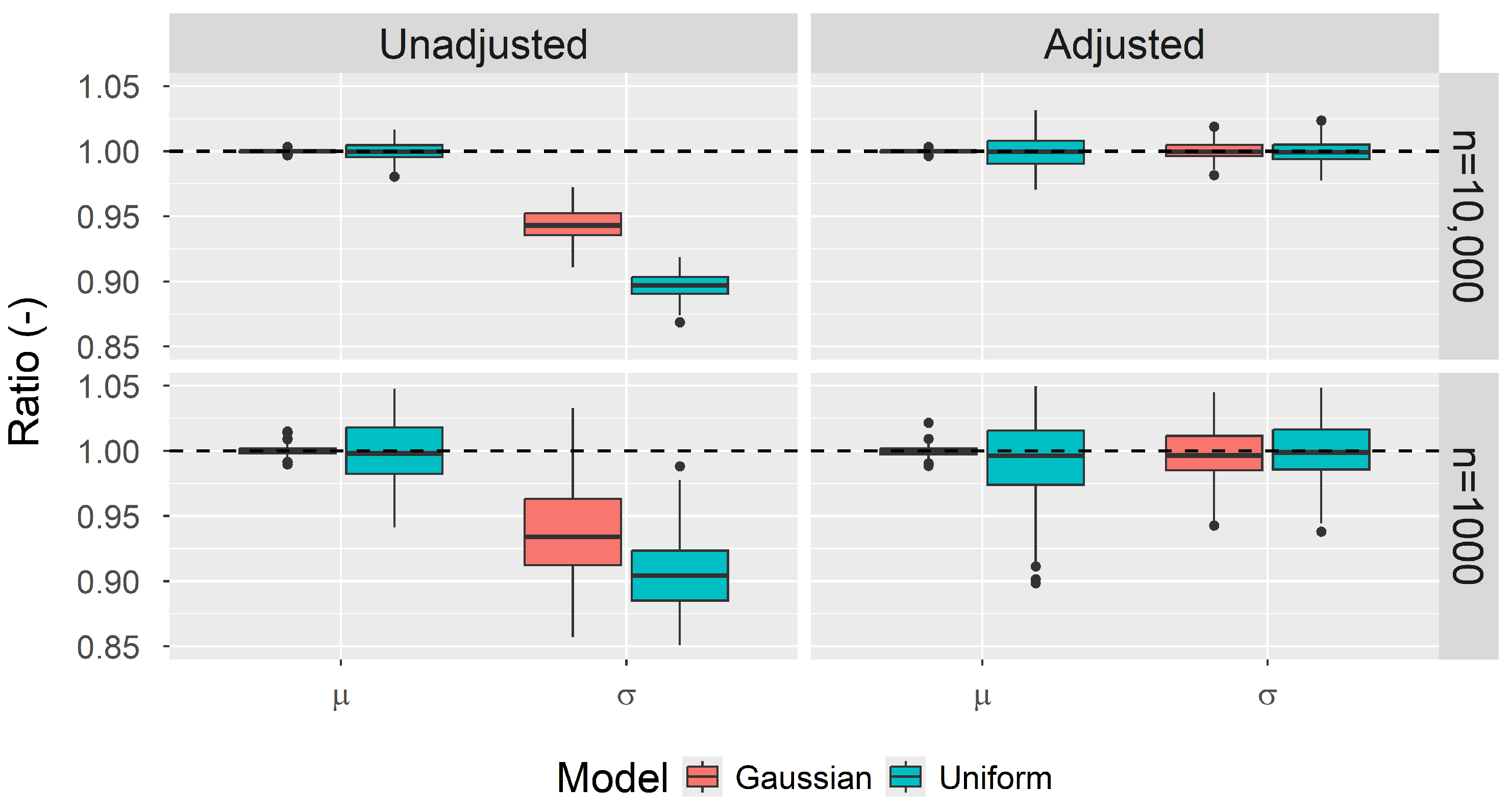
4.2. Results
5. Applications
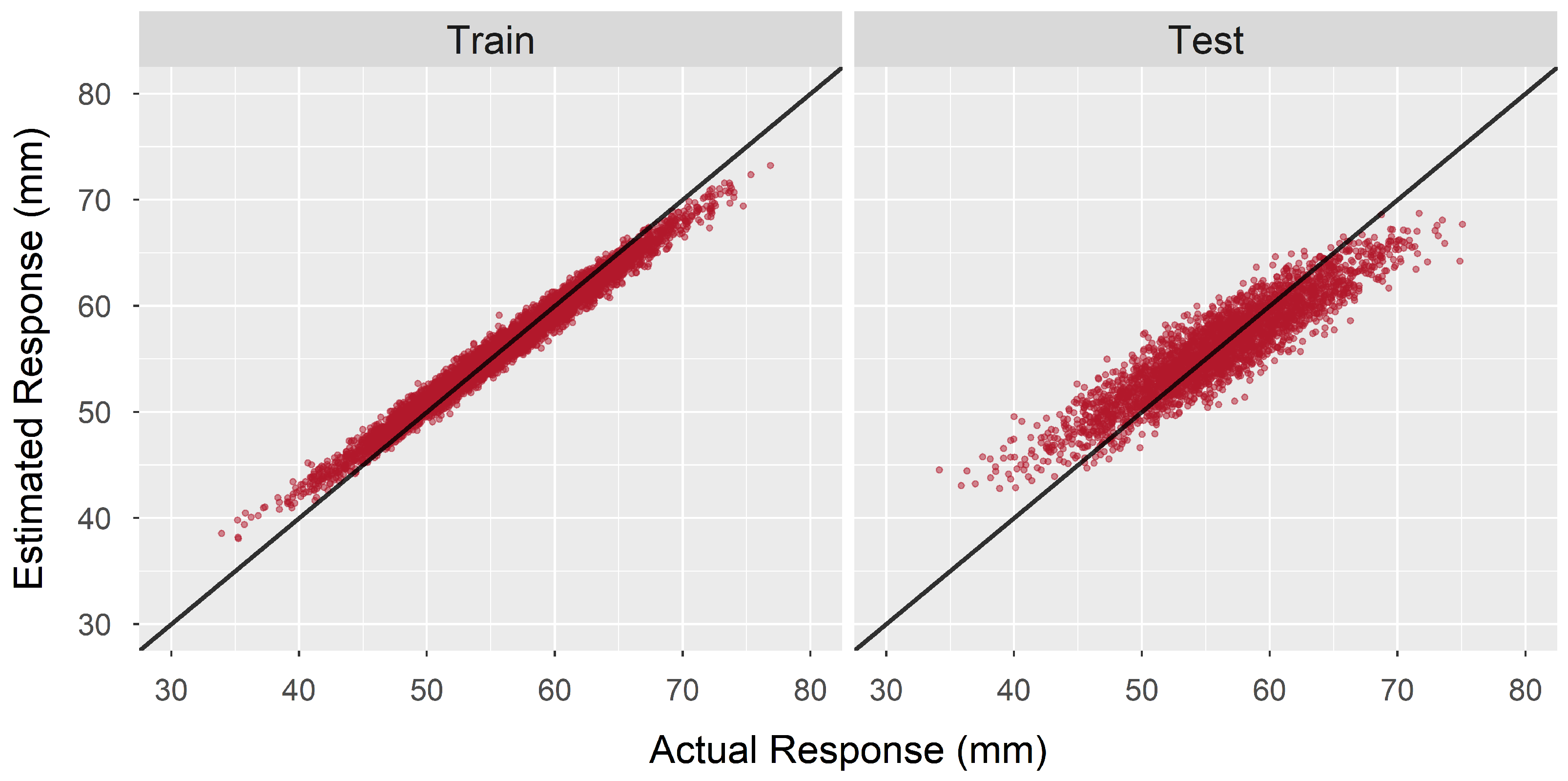
5.1. Depth-to-Load Conversion Model
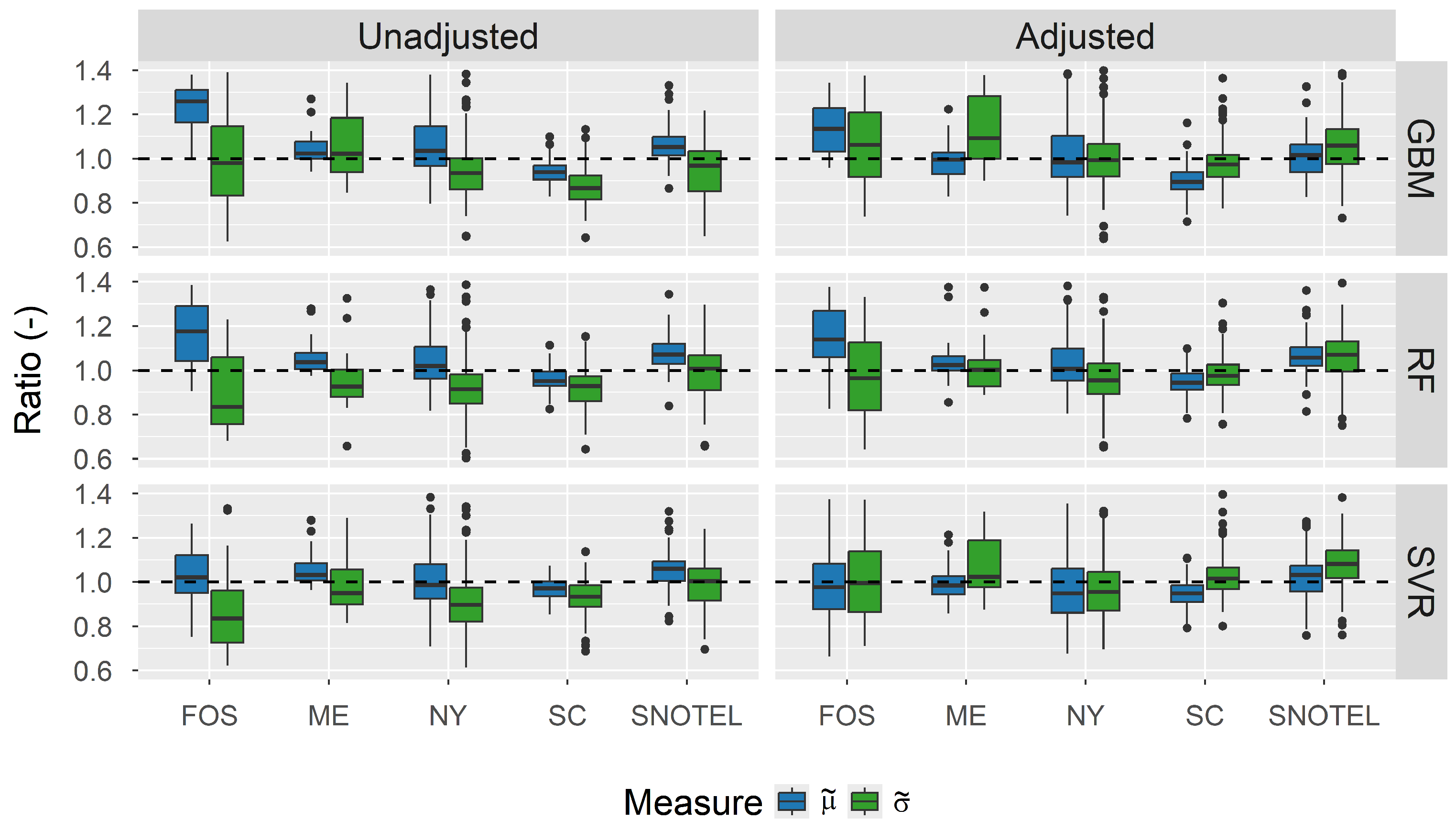
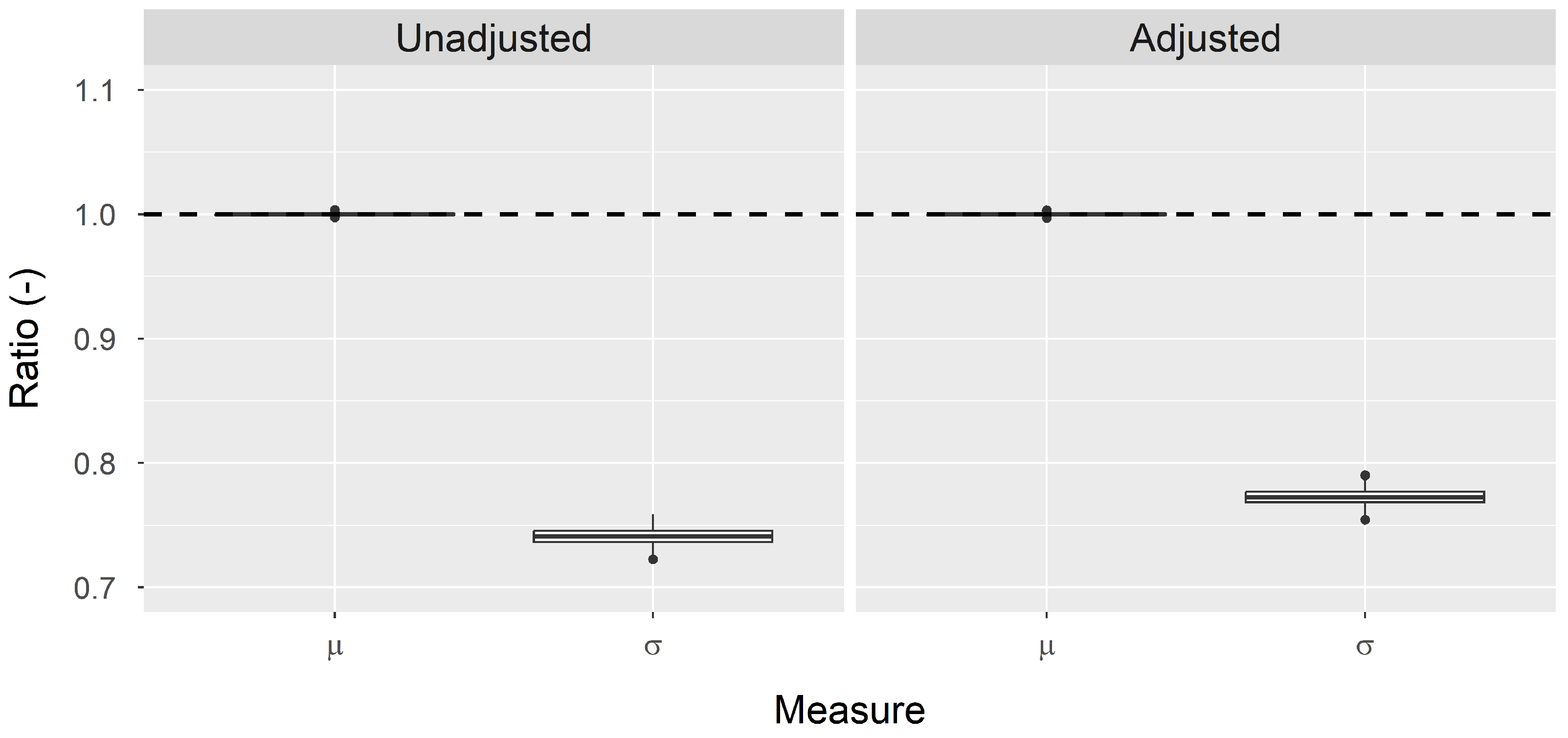
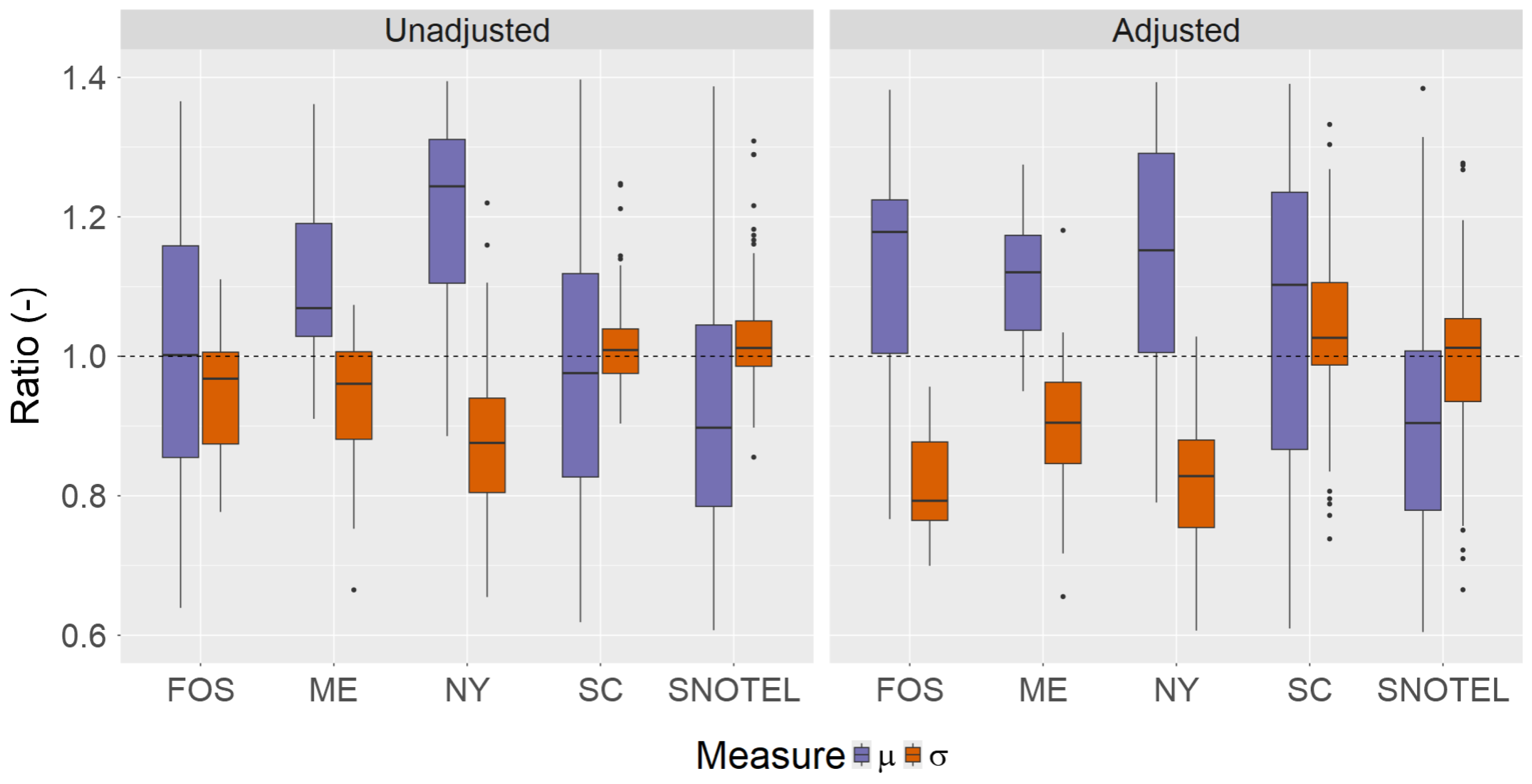
5.2. Bias Correction in Snow Load Distribution
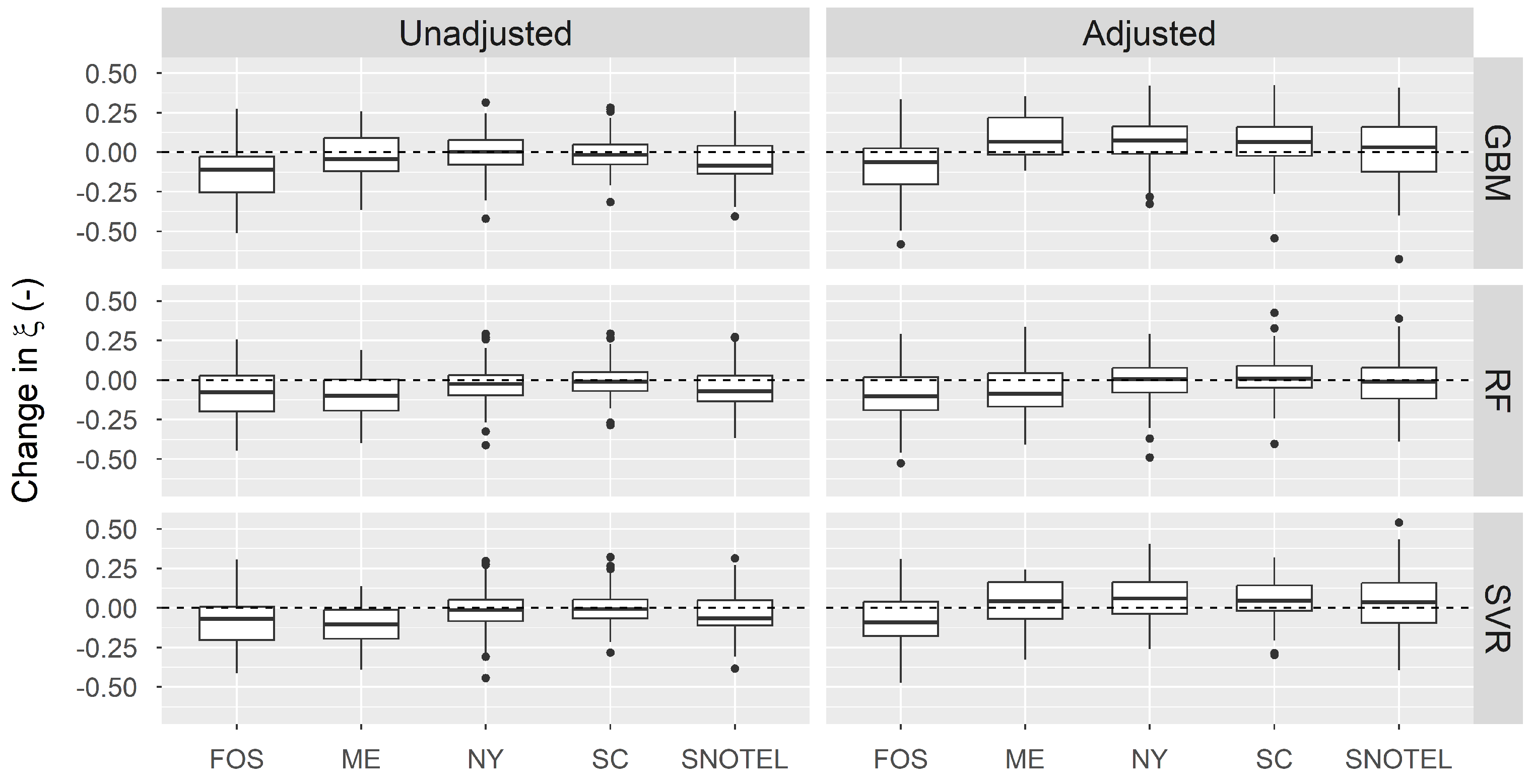
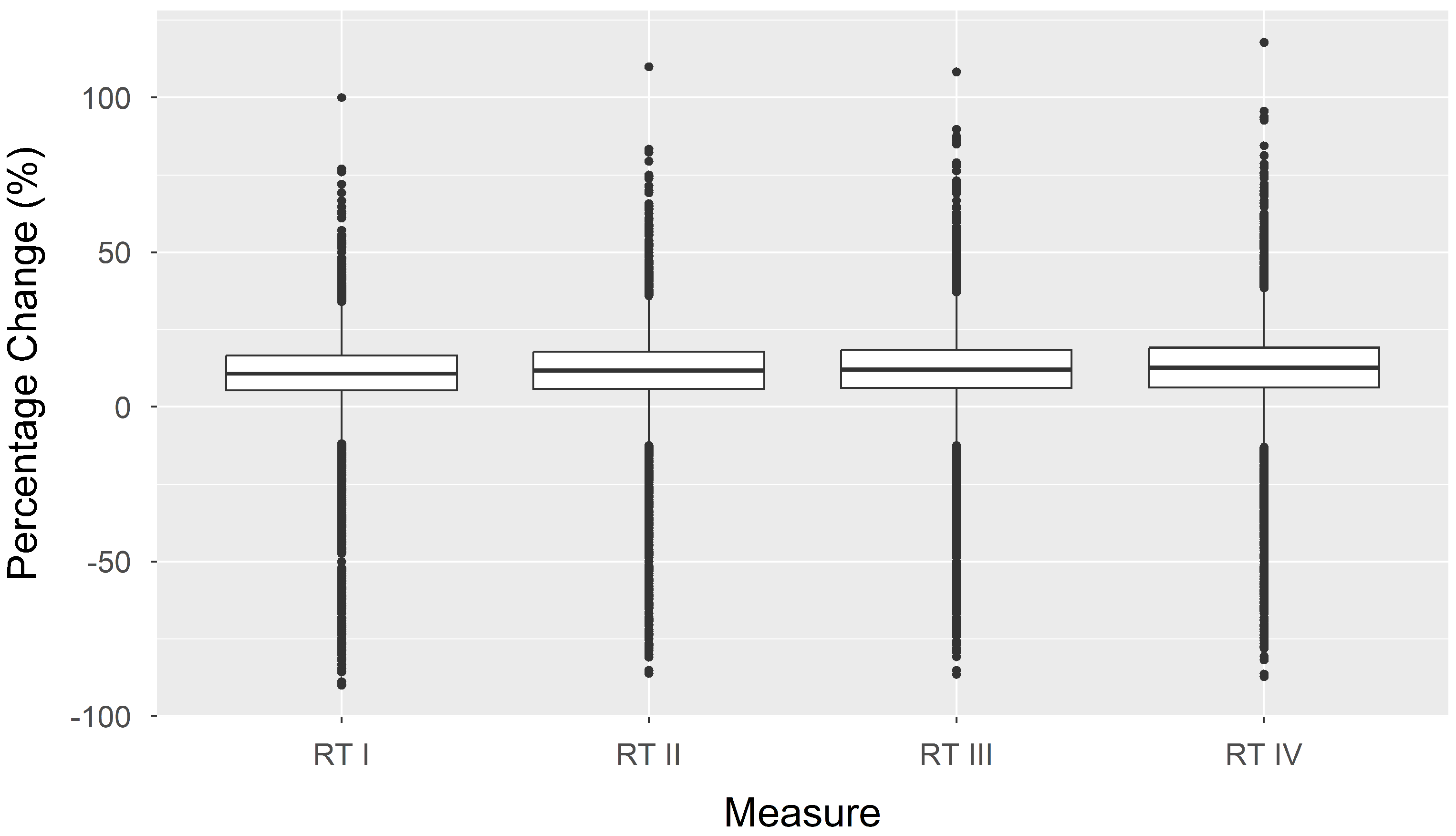
5.3. Reliability-Targeted Load (RTL) Results after Bias Correction
5.4. Limitations
6. Conclusions
Supplementary Materials
Author Contributions
Funding
Institutional Review Board Statement
Informed Consent Statement
Data Availability Statement
Conflicts of Interest
Abbreviations
| ASCE | American Society of Civil Engineers |
| BM | Block Maxima |
| COOP | Cooperative Observer Network |
| CONUS | Conterminous United States |
| CDF | Cumulative Distribution Function |
| ECDF | Empirical Cumulative Distribution Function |
| FOS | First-Order Stations |
| GEV | Generalized extreme value |
| GP | Generalized Pareto |
| GHCND | Global Historical Climatology Network—Daily |
| GBM | Gradient boosting machine |
| LRFD | Load And Resistance Factor Design |
| MAE | Mean Absolute Error |
| ME | Maine |
| MLE | Maximum likelihood estimation |
| MAD | Mean Absolute Deviation |
| MRI | Mean recurrence interval |
| ML | Maximum likelihood |
| NY | New York |
| NWS | National Weather Service |
| OSBF | One-step boosted forests |
| Probability Density Function | |
| RF | Random forests |
| RMSE | Root Mean Square Error |
| RTL | Reliability-targeted load |
| SWE | Snow water equivalent |
| SNODAS | Snow Data Assimilation System |
| SNOTEL | Snowpack Telemetry |
| SVR | Support vector regression |
| SC | Snow Course |
| SNWD | Snow depth |
| UA | University Of Arizona |
| WESD | Water Equivalent of Snow on the Ground |
| U.S. | United States |
References
- Al-Rubaye, S.; Maguire, M.; Bean, B. Design ground snow loads: Historical perspective and state of the art. J. Struct. Eng. 2022, 148, 03122001. [Google Scholar] [CrossRef]
- National Center for Atmospheric Research. The Climate Data Guide: ERA-Interim. 2022. Available online: https://climatedataguide.ucar.edu/climate-data/era-interim (accessed on 7 November 2022).
- Jonas, T.; Marty, C.; Magnusson, J. Estimating the snow water equivalent from snow depth measurements in the Swiss Alps. J. Hydrol. 2009, 378, 161–167. [Google Scholar] [CrossRef]
- Sturm, M.; Taras, B.; Liston, G.E.; Derksen, C.; Jonas, T.; Lea, J. Estimating snow water equivalent using snow depth data and climate classes. J. Hydrometeorol. 2010, 11, 1380–1394. [Google Scholar] [CrossRef]
- McCreight, J.L.; Small, E.E. Modeling bulk density and snow water equivalent using daily snow depth observations. Cryosphere 2014, 8, 521–536. [Google Scholar] [CrossRef]
- Wheeler, J.; Bean, B.; Maguire, M. Creating a universal depth-to-load conversion technique for the conterminous United States using random forests. J. Cold Reg. Eng. 2022, 36, 04021019. [Google Scholar] [CrossRef]
- Ross, S. A First Course in Probability; Pearson: Upper Saddle River, NJ, USA, 2010; pp. 333–348. [Google Scholar]
- Cho, E.; Jacobs, J.M. Extreme value snow water equivalent and snowmelt for infrastructure design over the contiguous United States. Water Resour. Res. 2020, 56, e2020WR028126. [Google Scholar] [CrossRef]
- R Core Team. R: A Language and Environment for Statistical Computing; R Foundation for Statistical Computing: Vienna, Austria, 2024. [Google Scholar]
- Wickham, H.; Averick, M.; Bryan, J.; Chang, W.; McGowan, L.D.; François, R.; Grolemund, G.; Hayes, A.; Henry, L.; Hester, J.; et al. Welcome to the tidyverse. J. Open Source Softw. 2019, 4, 1686. [Google Scholar] [CrossRef]
- Kuhn, M. Building Predictive Models in R Using the caret Package. J. Stat. Softw. 2008, 28, 1–26. [Google Scholar] [CrossRef]
- Kenneth, K. Distfixer: Distribution Bias Correction Using Residual Bootstrap. GitHub Repository. 2023. Available online: https://github.com/Kinekenneth48/distfixer (accessed on 7 November 2022).
- Gilleland, E.; Katz, R.W. extRemes 2.0: An Extreme Value Analysis Package in R. J. Stat. Softw. 2016, 72, 1–39. [Google Scholar] [CrossRef]
- Delignette-Muller, M.L.; Dutang, C. fitdistrplus: An R Package for Fitting Distributions. J. Stat. Softw. 2015, 64, 1–34. [Google Scholar] [CrossRef]
- Pavia, J.M. Testing Goodness-of-Fit with the Kernel Density Estimator: GoFKernel. J. Stat. Softw. Code Snippets 2015, 66, 1–27. [Google Scholar] [CrossRef]
- R package version 3.4.2. code by Richard, A.; Becker, O.S.; version by Brownrigg, R. Enhancements by Minka, T.P.; Deckmyn, A. maps: Draw Geographical Maps. 2023. Available online: https://CRAN.R-project.org/package=maps (accessed on 27 June 2024).
- Rinker, T.W.; Kurkiewicz, D. Pacman: Package Management for R, version 0.5.0.; Buffalo: New York, NY, USA, 2018; Available online: http://github.com/trinker/pacman (accessed on 7 November 2022).
- Wright, M.N.; Ziegler, A. ranger: A Fast Implementation of Random Forests for High Dimensional Data in C++ and R. J. Stat. Softw. 2017, 77, 1–17. [Google Scholar] [CrossRef]
- Bengtsson, H. A Unifying Framework for Parallel and Distributed Processing in R using Futures. R J. 2021, 13, 208–227. [Google Scholar] [CrossRef]
- Ridgeway, G.; Developers, G. gbm: Generalized Boosted Regression Models; R Package Version 2.2.2. Available online: https://CRAN.R-project.org/package=gbm (accessed on 7 November 2022).
- Karatzoglou, A.; Smola, A.; Hornik, K.; Zeileis, A. kernlab—An S4 Package for Kernel Methods in R. J. Stat. Softw. 2004, 11, 1–20. [Google Scholar] [CrossRef]
- Hijmans, R.J. raster: Geographic Data Analysis and Modeling; R Package Version 3.6-26. Available online: https://CRAN.R-project.org/package=raster (accessed on 7 November 2022).
- Pebesma, E.; Bivand, R. Spatial Data Science: With Applications in R; Chapman and Hall/CRC: Boca Raton, FL, USA, 2023; p. 352. [Google Scholar] [CrossRef]
- Zhang, G.; Lu, Y. Bias-corrected random forests in regression. J. Appl. Stat. 2012, 39, 151–160. [Google Scholar] [CrossRef]
- Hooker, G.; Mentch, L. Bootstrap bias corrections for ensemble methods. Stat. Comput. 2016, 28, 77–86. [Google Scholar] [CrossRef]
- Breiman, L. Using Adaptive Bagging to Debias Regressions; Technical Report 547; Statistics Dept. UCB: Berkeley, CA, USA, 1999; Available online: https://www.stat.berkeley.edu/users/breiman/adaptbag99.pdf (accessed on 7 November 2022).
- Ghosal, I.; Hooker, G. Boosting random forests to reduce bias; one-step boosted forest and its variance estimate. J. Comput. Graph. Stat. 2020, 30, 493–502. [Google Scholar] [CrossRef]
- Song, J. Bias corrections for random forest in regression using residual rotation. J. Korean Stat. Soc. 2015, 44, 321–326. [Google Scholar] [CrossRef]
- Belitz, K.; Stackelberg, P. Evaluation of six methods for correcting bias in estimates from ensemble tree machine learning regression models. Environ. Model. Softw. 2021, 139, 105006. [Google Scholar] [CrossRef]
- Broxton, P.D.; Dawson, N.; Zeng, X. Linking snowfall and snow accumulation to generate spatial maps of SWE and snow depth. Earth Space Sci. 2016, 3, 246–256. [Google Scholar] [CrossRef]
- Barrett, A.P. National Operational Hydrologic Remote Sensing Center Snow Data Assimilation System (SNODAS) Products at NSIDC; Technical Report 11; National Snow and Ice Data Center, Cooperative Institute for Research in Environmental Sciences: Boulder, CO, USA, 2003; Available online: https://nsidc.org/sites/default/files/nsidc_special_report_11.pdf (accessed on 7 November 2022).
- Carroll, T.; Cline, D.; Fall, G.; Nilsson, A.; Li, L.; Rost, A. NOHRSC operations and the simulation of snow cover properties for the coterminous US. In Proceedings of the Annual Meeting of the Western Snow Conference, Sun Valley, ID, USA, 17–19 April 2001; pp. 1–14. Available online: https://www.nohrsc.noaa.gov/technology/papers/wsc2001/wsc2001.pdf (accessed on 7 November 2022).
- Wood, A.W.; Leung, L.R.; Sridhar, V.; Lettenmaier, D.P. Hydrologic implications of dynamical and statistical approaches to downscaling climate model outputs. Clim. Chang. 2004, 62, 189–216. [Google Scholar] [CrossRef]
- Boé, J.; Terray, L.; Habets, F.; Martin, E. Statistical and dynamical downscaling of the Seine basin climate for hydro-meteorological studies. Int. J. Climatol. 2007, 27, 1643–1655. [Google Scholar] [CrossRef]
- Ashfaq, M.; Bowling, L.C.; Cherkauer, K.; Pal, J.S.; Diffenbaugh, N.S. Influence of climate model biases and daily-scale temperature and precipitation events on hydrological impacts assessment: A case study of the United States. J. Geophys. Res. 2010, 115, D14. [Google Scholar] [CrossRef]
- Haerter, J.O.; Hagemann, S.; Moseley, C.; Piani, C. Climate model bias correction and the role of timescales. Hydrol. Earth Syst. Sci. 2011, 15, 1065–1079. [Google Scholar] [CrossRef]
- Piani, C.; Haerter, J.O.; Coppola, E. Statistical bias correction for daily precipitation in regional climate models over Europe. Theor. Appl. Climatol. 2009, 99, 187–192. [Google Scholar] [CrossRef]
- Ines, A.V.; Hansen, J.W. Bias correction of daily GCM rainfall for crop simulation studies. Agric. For. Meteorol. 2006, 138, 44–53. [Google Scholar] [CrossRef]
- Lakshmanan, V.; Gilleland, E.; McGovern, A.; Tingley, M. Machine Learning and Data Mining Approaches to Climate Science; Springer: Berlin/Heidelberg, Germany, 2015; Available online: https://link.springer.com/book/10.1007/978-3-319-17220-0 (accessed on 7 November 2022).
- ASCE 7-22. Minimum Design Loads and Associated Criteria for Buildings and Other Structures, ASCE/SEI 7-22 ed.; American Society of Civil Engineers: Reston, VA, USA, 2022; Available online: https://ascelibrary.org/doi/abs/10.1061/9780784415788 (accessed on 7 November 2022).
- Ellingwood, B.; Galambos, T.V.; MacGregor, J.G.; Cornell, C.A. Development of a Probability Based Load Criterion for American National Standard A58: Building Code Requirements for Minimum Design Loads in Buildings and Other Structures; US Department of Commerce, National Bureau of Standards: Washington, DC, USA, 1980; Volume 13. Available online: https://nvlpubs.nist.gov/nistpubs/Legacy/SP/nbsspecialpublication577.pdf (accessed on 7 November 2022).
- Ellingwood, B.; MacGregor, J.G.; Galambos, T.V.; Cornell, C.A. Probability based load criteria: Load factors and load combinations. J. Struct. Div. 1982, 108, 978–997. [Google Scholar] [CrossRef]
- Galambos, T.V.; Ellingwood, B.; MacGregor, J.G.; Cornell, C.A. Probability based load criteria: Assessment of current design practice. J. Struct. Div. 1982, 108, 959–977. [Google Scholar] [CrossRef]
- DeBock, D.J.; Liel, A.B.; Harris, J.R.; Ellingwood, B.R.; Torrents, J.M. Reliability-based design snow loads. I: Site-specific probability models for ground snow loads. J. Struct. Eng. 2017, 143, 04017046. [Google Scholar] [CrossRef]
- Liel, A.B.; DeBock, D.J.; Harris, J.R.; Ellingwood, B.R.; Torrents, J.M. Reliability-based design snow loads. II: Reliability assessment and mapping procedures. J. Struct. Eng. 2017, 143, 04017047. [Google Scholar] [CrossRef]
- Bean, B.; Maguire, M.; Sun, Y.; Wagstaff, J.; Al-Rubaye, S.A.; Wheeler, J.; Jarman, S.; Rogers, M. The 2020 National Snow Load Study; Technical Report 276; Utah State University Department of Mathematics and Statistics: Logan, UT, USA, 2021. [Google Scholar] [CrossRef]
- Bean, B.; Maguire, M.; Sun, Y. The Utah snow load study. Civ. Environ. Eng. Fac. Publ. 2018, 3589. Available online: https://digitalcommons.usu.edu/cee_facpub/3589 (accessed on 7 November 2022).
- Ellingwood, B.; Redfield, R. Ground snow loads for structural design. J. Struct. Eng. 1983, 109, 950–964. [Google Scholar] [CrossRef]
- Mo, H.; Dai, L.; Fan, F.; Che, T.; Hong, H. Extreme snow hazard and ground snow load for China. Nat. Hazards 2016, 84, 2095–2120. [Google Scholar] [CrossRef]
- Mo, H.M.; Ye, W.; Hong, H.P. Estimating and mapping snow hazard based on at-site analysis and regional approaches. Nat. Hazards 2022, 111, 2459–2485. [Google Scholar] [CrossRef]
- Structural Engineers Association of Colorado. Colorado Ground Snow Loads; SEAC: Colorado, CO, USA, 2007. [Google Scholar]
- Efron, B. Bootstrap methods: Another look at the jackknife. Ann. Stat. 1979, 7, 1–26. [Google Scholar] [CrossRef]
- Diciccio, T.J.; Romano, J.P. A review of bootstrap confidence intervals. J. R. Stat. Soc. Ser. B (Methodol.) 1988, 50, 338–354. Available online: https://www.jstor.org/stable/2345699 (accessed on 7 November 2022). [CrossRef]
- Davison, A.C.; Hinkley, D.V. Bootstrap Methods and Their Application; Cambridge University Press: Cambridge, UK, 1997; Available online: https://www.cambridge.org/core/books/bootstrap-methods-and-their-application/ED2FD043579F27952363566DC09CBD6A (accessed on 7 November 2022).
- Hall, P. The Bootstrap and Edgeworth Expansion; Springer Science and Business Media: New York, NY, USA, 1992; Available online: https://people.eecs.berkeley.edu/~jordan/sail/readings/edgeworth.pdf (accessed on 7 November 2022).
- Kim, J.H. Forecasting autoregressive time series with bias-corrected parameter estimators. Int. J. Forecast. 2003, 19, 493–502. [Google Scholar] [CrossRef]
- Franco, G.C.; Reisen, V.A. Bootstrap approaches and confidence intervals for stationary and non-stationary long-range dependence processes. Phys. A Stat. Mech. Its Appl. 2007, 375, 546–562. [Google Scholar] [CrossRef]
- Engsted, T.; Pedersen, T. Bias-correction in vector autoregressive models: A simulation study. Econometrics 2014, 2, 45–71. [Google Scholar] [CrossRef]
- Palm, B.G.; Bayer, F.M. Bootstrap-based inferential improvements in beta autoregressive moving average model. Commun. Stat.- Comput. 2017, 47, 977–996. [Google Scholar] [CrossRef]
- De Vos, I.; Everaert, G.; Ruyssen, I. Bootstrap-based bias correction and inference for dynamic panels with fixed effects. Stata J. 2015, 15, 986–1018. [Google Scholar] [CrossRef]
- Everaert, G.; Pozzi, L. Bootstrap-based bias correction for dynamic panels. J. Econ. Dyn. Control 2007, 31, 1160–1184. [Google Scholar] [CrossRef]
- Kim, J. Bias-corrected bootstrap inference for regression models with autocorrelated errors. Econ. Bull. 2005, 3, 1–8. Available online: http://www.accessecon.com/pubs/EB/2005/Volume3/EB-05C20017A.pdf (accessed on 7 November 2022).
- Ferrari, S.L.; Cribari-Neto, F. On bootstrap and analytical bias corrections. Econ. Lett. 1998, 58, 7–15. [Google Scholar] [CrossRef]
- Menne, M.; Durre, I.; Korzeniewski, B.; Vose, R.; Gleason, B.; Houston, T. Global Historical Climatology Network—Daily (GHCN-Daily); Version 3.26; NOAA: Silver Spring, MD, USA, 2012. [Google Scholar] [CrossRef]
- Natural Resources Conservation Service. Snow Telemetry (SNOTEL) and Snow Course Data and Products; NRCS: Washington, DC, USA, 2020. Available online: https://www.wcc.nrcs.usda.gov/snow/ (accessed on 7 November 2022).
- Maine Geological Survey. Maine Snow Survey Data; Maine Geological Survey: Augusta, ME, USA, 2020; Available online: https://mgs-maine.opendata.arcgis.com/datasets/maine-snow-survey-data (accessed on 7 November 2022).
- Northeast Regional Climate Center. New York Snow Survey Data; Data Obtained through Personal Correspondence with Northeast Regional Climate Center; NRCC-Cornell University: Ithaca, NY, USA, 2020; Available online: http://www.nrcc.cornell.edu/ (accessed on 7 November 2022).
- Wheeler, J.; Bean, B.; Maguire, M. Supplementary Files for “Creating a Universal Depth-To-Load Conversion Technique for the Conterminous United States using Random Forests”; Utah State University: Logan, UT, USA, 2021; Volume 1001, p. 48109. [Google Scholar] [CrossRef]
- Zhang, H.; Nettleton, D.; Zhu, Z. Regression-enhanced random forests. In Proceedings of the JSM Proceedings, American Statistical Association, Alexandria, VA, USA, 23 April 2019; Section on Statistical Learning and Data Science. pp. 636–647. Available online: https://arxiv.org/pdf/1904.10416.pdf (accessed on 7 November 2022).


| 98th Percentile | 99th Percentile | |||
|---|---|---|---|---|
| Extreme Event | Relative Increase (%) (from ) | Extreme Event | Relative Increase (%) (from ) | |
| 1 | 7.8 | 10.24 | ||
| 1.1 | 9.57 | 21.1 | 12.9 | 26 |
| 1.2 | 11.8 | 51.2 | 16.3 | 59.1 |
| 1.3 | 14.4 | 84.6 | 20.6 | 100.1 |
| Uniform Model | Gaussian Model | ||||||||
|---|---|---|---|---|---|---|---|---|---|
| COV | Bias | COV | Bias | ||||||
| n = 10,000 | Unadjusted | 0.01 | 0.01 | 1.00 | 0.90 | 0.00 | 0.01 | 1.00 | 0.94 |
| Adjusted | 0.01 | 0.01 | 1.00 | 1.00 | 0.00 | 0.01 | 1.00 | 1.00 | |
| n = 1000 | Unadjusted | 0.04 | 0.04 | 1.00 | 0.90 | 0.00 | 0.04 | 1.00 | 0.94 |
| Adjusted | 0.03 | 0.03 | 1.00 | 1.00 | 0.00 | 0.02 | 1.00 | 1.00 | |
| Climate Variables | |||
|---|---|---|---|
| Name | Description | Units | Variable |
| SD | Snow Depth | mm | |
| SWE | Snow Water Equivalent | mm | s |
| MCMT | Mean Coldest Month Temperature | °C | |
| MWMT | Mean Warmest Month Temperature | °C | |
| TD | MWMT–MCMT | °C | |
| PPTWT | Sum of Winter Precipitation (December–February) | ||
| Non-Climate Variables | |||
| D2C | Distance to Coast | m | |
| ELEV | Elevation | m | E |
| SMONTH | Month of Max Depth (1 October, 9 June) | ||
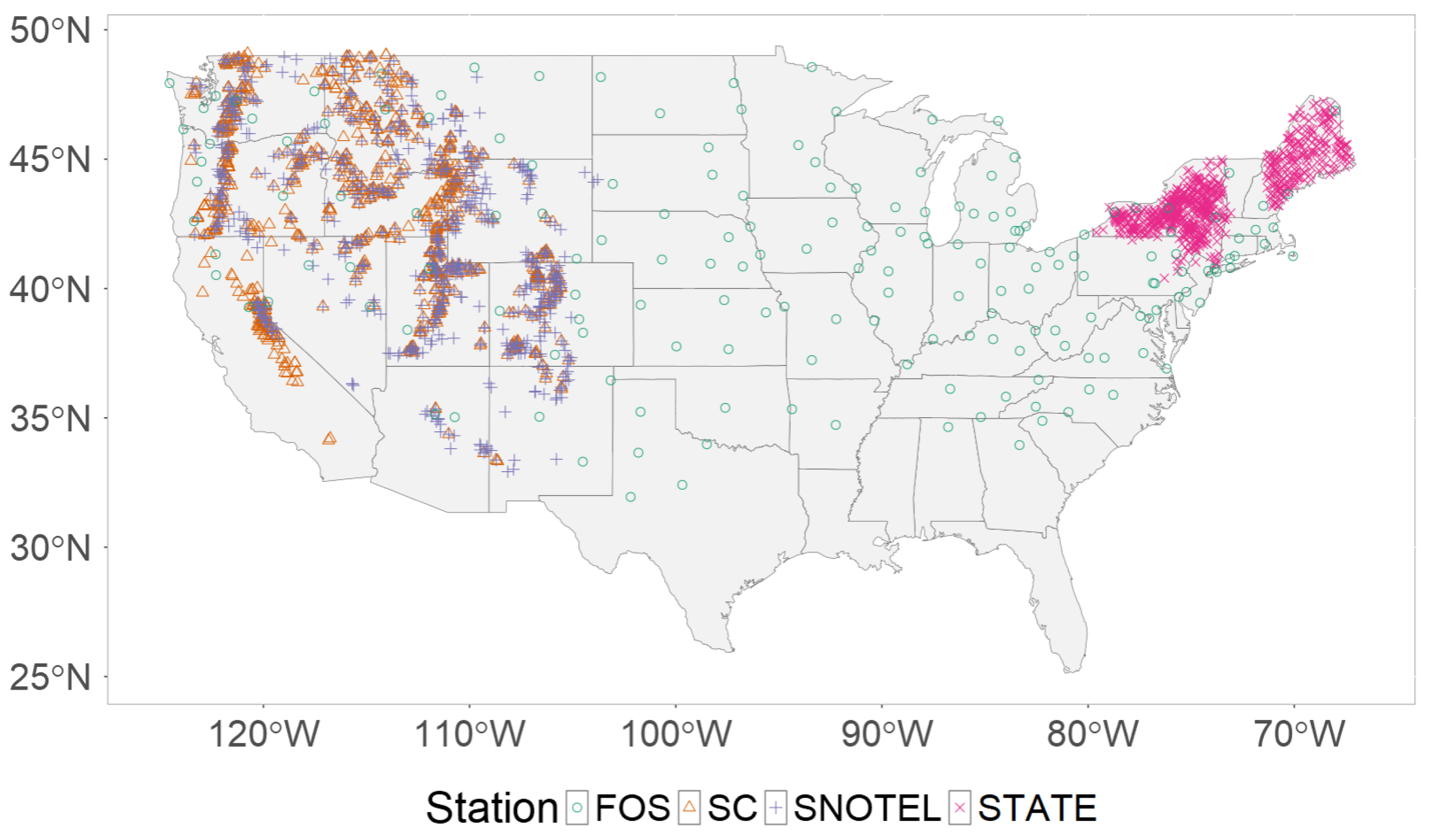
| Network | Name | Number of Weather Stations |
|---|---|---|
| FOS | First-Order Stations | 46 |
| ME | Maine State Network | 23 |
| NY | New York State Network | 122 |
| SC | Snow Course | 144 |
| SNOTEL | Snowpack Telemetry | 74 |
Disclaimer/Publisher’s Note: The statements, opinions and data contained in all publications are solely those of the individual author(s) and contributor(s) and not of MDPI and/or the editor(s). MDPI and/or the editor(s) disclaim responsibility for any injury to people or property resulting from any ideas, methods, instructions or products referred to in the content. |
© 2024 by the authors. Licensee MDPI, Basel, Switzerland. This article is an open access article distributed under the terms and conditions of the Creative Commons Attribution (CC BY) license (https://creativecommons.org/licenses/by/4.0/).
Share and Cite
Pomeyie, K.; Bean, B. Bootstrap Methods for Bias-Correcting Probability Distribution Parameters Characterizing Extreme Snow Accumulations. Glacies 2024, 1, 35-56. https://doi.org/10.3390/glacies1010004
Pomeyie K, Bean B. Bootstrap Methods for Bias-Correcting Probability Distribution Parameters Characterizing Extreme Snow Accumulations. Glacies. 2024; 1(1):35-56. https://doi.org/10.3390/glacies1010004
Chicago/Turabian StylePomeyie, Kenneth, and Brennan Bean. 2024. "Bootstrap Methods for Bias-Correcting Probability Distribution Parameters Characterizing Extreme Snow Accumulations" Glacies 1, no. 1: 35-56. https://doi.org/10.3390/glacies1010004
APA StylePomeyie, K., & Bean, B. (2024). Bootstrap Methods for Bias-Correcting Probability Distribution Parameters Characterizing Extreme Snow Accumulations. Glacies, 1(1), 35-56. https://doi.org/10.3390/glacies1010004