Review

Geophysical and Remote Sensing Methods for Locating Orphaned Oil and Gas Wells: An Overview and Accessibility of Smartphone Magnetometry


1
Department of Earth Sciences, Binghamton University, Binghamton, NY 13902, USA
2
School of Systems Science and Industrial Engineering, Binghamton University, Binghamton, NY 13902, USA
*
Author to whom correspondence should be addressed.
Submission received: 28 May 2026 / Revised: 26 June 2026 / Accepted: 14 July 2026 / Published: 18 July 2026

Abstract

Approximately 140,000 of the estimated one million orphaned wells in the United States have been documented, leaving the majority unaccounted for. These undocumented wells emit atmospheric methane and allow for hydrocarbon and brine groundwater migration. Many wells are difficult to locate due to subsequent covering or the removal of their surface casing, making manual identification impractical. Professional geophysical and remote sensing methods to locate orphaned wells are financially and technically inaccessible to the public, limiting their scalability. Accessible methods for identifying wells have been introduced, including drone and smartphone surveys, as well as artificial intelligence. Smartphone magnetometers are a low-cost alternative for locating steel-cased wells with greater spatial resolution than aerial magnetometry and portability than traditional handheld magnetometers. This study reviews existing techniques for orphaned well detection and presents smartphone magnetometry as a reliable well location tool. The resulting data from dynamic smartphone magnetic surveys exhibited limited background noise and a more precise well target than professional aerial surveys, while lowering cost and operational difficulty. Diffusion modeling generated synthetic data near the well, improving the resolution of anomalous magnetic readings. Smartphone surveys require minimal expertise, finances, and equipment, representing a simple method for a large-scale effort to address orphaned wells.

1. Introduction

Since the origins of the oil and gas industry with the success of the 1859 Drake Well in Pennsylvania, millions of exploration and extraction wells have been drilled throughout the United States. Modern regulations for upstream oil and gas operations developed as the industry matured throughout the early to mid-20th century, meaning nearly a century of unregulated drilling practices took place that left behind wells as open holes or pipes once they were deemed dry, or no longer economically profitable [1]. Acting as conduits into the subsurface, unplugged wells allow for methane, hydrocarbons, brine, metals, and volatile organic compounds to migrate into the local groundwater and atmosphere as their casing corrodes over time [2,3,4,5,6,7]. For example, methane leakage from orphaned oil and gas wells is estimated to contribute 300 kt of atmospheric methane annually [8]. While plugged wells emit < 1 g CH4/hr, unplugged orphaned wells may leak anywhere from 5–10 g CH4/hr [2,4,9,10,11] to >100 g CH4/hr [12]. A total of 57% of the U.S. abandoned oil and gas well population are estimated to be unplugged, which passively contributes 1% of total annual anthropogenic methane emissions [8].
The U.S. Environmental Protection Agency (U.S. EPA) estimates that 3.9 million abandoned oil and gas wells exist throughout the country [8]. Nearly one million of these wells are estimated to be orphaned, meaning they have been insufficiently or not plugged, with no documentation of their owner [8]. However, recent databases from 30 state records contain 141,959 documented orphaned wells [13]. This suggests that less than a quarter of presently orphaned wells have been accounted for. With most documented orphaned wells located in the nation’s primary aquifers [14] and emitting large amounts of methane into the atmosphere, there has been a growing interest in the past decade in locating and plugging these wells to diminish their environmental impacts. The U.S. federal government’s 2021 Infrastructure Investment and Jobs Act (IIJA) Section 40,601 granted USD 4.677 billion to federal, state, and tribal programs to improve the efficiency of plugging and remediating orphaned wells. As of June 2025, 10,257 documented orphaned wells were plugged across 26 states [15]. As these programs focus on the plugging and restoration of known orphaned wells, it is crucial that reliable methods for locating undocumented orphaned wells are developed for nationwide use.
With a median plugging and reclamation rate of roughly USD 55,000 per well in the U.S. [16], identifying the most resource-efficient method for pinpointing the exact location of a well is necessary (Table 1). For such a large-scale problem that exists on both public and private lands, accessible methods for detecting orphaned wells will allow for a larger audience to efficiently collect high-resolution data nationwide, rather than relying on a limited group of technical experts. The variety of geophysical and remote sensing methods for detecting orphaned wells, such as magnetometry, electrical resistivity, optical imagery, and Light Detection and Ranging (LiDAR), provides diverse information on their location and interactions with the environment [17,18,19,20]. This grants surveyors the flexibility to pursue any combination of techniques that suit their investigation needs and availability of resources. Still, technical methods remain inaccessible to the public due to the cost of equipment and technical expertise required. Most modern smartphones contain a hall-effect magnetometer to assist in user navigation using the Global Positioning System (GPS). Researchers have begun using these accessible and portable sensors for subsurface magnetic investigations [21,22], including the detection of orphaned wells [23]. As a low-cost instrument that is owned by many people worldwide, smartphones demonstrate the potential to fill gaps in generalizability and data collection efficiency that can arise when surveying with professional magnetometers [20,22,23]. However, there has been a lack of research on the potential for smartphone magnetometers to detect orphaned wells with unsupervised survey methods such as walking or hiking with no predefined survey grids. If successful, large-scale data collected by smartphone users across the country could eliminate the reliance on professional geophysicists to gather magnetic data for locating orphaned wells. Cumulative smartphone data collected from citizens during outdoor excursions and those intentionally searching for orphaned wells could provide a cost-efficient and low-effort avenue for collecting magnetic data on a nationwide scale.
The proof-of-concept surveys in this study aim to investigate the performance of unsupervised walking smartphone magnetometer surveying, potentially the most accessible technique thus far, as an alternative to professional geophysical methods for locating orphaned wells. To test this, smartphone magnetometers are deployed to detect a documented, abandoned gas well with no evidence at the surface of its location. The results of these surveys suggest that the magnetic signature of abandoned and orphaned wells can be detected in minimally processed smartphone data that was collected in symmetrical and asymmetrical survey grids, further implying that this method is appropriate for users of varying technical expertise. Given this, smartphone magnetometers are capable of being used by the large population of smartphone users to detect the magnetic signature of orphaned wells on a nationwide scale.

2. Geophysical and Remote Sensing Characterization of Orphaned Wells

Orphaned wells stand out in magnetic investigations due to their long steel casing that is installed vertically into the subsurface as part of the drilling and completion stage. The long and vertical orientation of these wells produces an intense, concentrated magnetic monopole anomaly that is distinct from dipolar signals caused by local magnetic objects [18,24,25,26,27]. This signal is centered at the location of the well, providing an effective target for locating wells with magnetic surveying [25,26]. The acute signal can be resolved at heights up to about 50 m above ground level (AGL), at which point dipole magnetic signals are attenuated [25,26]. However, as the steel deteriorates with time (i.e., rusting), the magnetic signature diminishes [28] and limits detectability to lower altitudes depending on sensor sensitivity [23,29]. As well infrastructure deteriorates over time or is not properly plugged, conduits are formed between the inside of the well and the subsurface formations. This allows for leftover brine and hydrocarbons to seep into the critical zone, including local groundwater and soil [30,31,32]. Brine contamination can increase the dissolved content of dissolved solids in subsurface fluid, inversely decreasing the electrical resistivity [33,34,35]. Conversely, increased pure hydrocarbon content increases the material’s electrical resistivity [36,37,38,39,40]. Additionally, if a well’s steel casing is present, the metallic material produces a strong low-resistivity signal that can dominate the electrical resistivity readings [41]. These changes in subsurface resistivity centered around the point of drilling provide clues to the location of an orphaned well [17,41]. Furthermore, surface footprints of orphaned wells can be found using visual imagery and LiDAR data. Leftover drilling infrastructure (e.g., wellheads, access roads, retention ponds) [42,43], soil subsidence caused by deteriorated well casing [27,28,29,30,31,32,33,34,35,36,37,38,39,40,41,42,43], and salt precipitation and vegetation decline from brine seepage [32,41] can be surface indicators of the presence of an undocumented well. The evolution of these surface remnants can be analyzed in historical maps and imagery, providing clues to when drilling may have taken place and to the state of potential environmental impacts [20,26,43].

3. Common Methods for Orphaned Well Detection

3.1. Ground-Based Methods

Collecting data at the surface, ground-based magnetometry has been widely used in many studies as an effective method for locating wells whose steel casing remains in the ground [25,29,42,43,44,45,46,47]. Surveyors have leveraged ground-based magnetometry to obtain a detailed view of broad magnetic anomalies found in aerial surveys [25,29,42,43]. Doing so, ground-based methods have revealed the location of wells with weaker magnetic signal caused by their deteriorating steel casing [43] or being covered with overlying material [29] that were missed by aerial surveying. Campbell et al., 2020 used smartphone magnetometers to locate vertically buried steel pipes in the shallow subsurface [22], which suggests that smartphones can detect the strong magnetic anomaly from orphaned wells despite their low sensitivity [23]. These surveys using professional and smartphone magnetometers have shown that ground-based methods can accurately pinpoint the location of steel-cased wells at various stages of deterioration and aging.
Electrical resistivity has been used to pinpoint orphaned wells by mapping low resistivity anomalies from their steel casing [41,48] and saline contamination plumes [41]. Using various electrode configurations, Saribudak et al., 2020 highlighted that electrical resistivity can be tailored to predominantly resolve either the location of the steel casing or contamination plume extent [41]. Electrical resistivity has proven useful for mapping the high resistivity of pure hydrocarbons leaking into groundwater [36,37,38,39,40], beach sediment [49], and soil [50,51,52,53]. These applications imply that electrical resistivity may provide a non-invasive method for characterizing the subsurface contamination of orphaned wells, especially for locating wells that are otherwise undetectable from the surface [41]. However, this method cannot distinguish whether the signal is related to a well casing or the brine leakage unless the location of the target well is predetermined.

3.2. Aerial Methods

Aeromagnetic surveying has become a common method for locating orphaned wells due to its ability to rapidly detect their steel casing [23,24,25,26,27,29,42,43,54,55]. Magnetometers flown at altitudes up to 50 m detect the intense magnetic signal from steel-cased wells while missing weaker signals from other sources [25,26,29,43,54]. As their strong magnetic anomaly sits directly above the well, aerial magnetometry can efficiently detect 1 to 1000 wells in a single survey [23,24,25,26,27,29,42,43,54]. Doing so, aerial magnetometry provides targets for the location of steel-cased wells, which has been shown to have a direct correlation to pinpointing high methane-emitting unplugged wells [54]. This time-efficient method rapidly narrows the focus for conducting further concentrated investigations of potential anomalies using ground-based methods, reducing the physical labor demand for surveyors and increasing the rate of documentation for wells throughout large regions [23,25,26,29,42,43,55].
Aerial LiDAR data has been used to provide complementary data to other geophysical methods (e.g., magnetometry) to highlight well-related surface features such as well retention ponds [42] and well subsidence [27,43]. As subsidence is common for deteriorated wood-cased wells, LiDAR can locate wells that provide no discernible magnetic signature [27,43]. Recent studies have applied aerial gas mapping LiDAR techniques to monitor atmospheric methane emissions from active upstream oil and gas production [56] and as a tool for active well location [25], suggesting that LiDAR can aid in continuous monitoring of environmental remediation of known wells and in detecting legacy wells drilled before modern regulations were established.

3.3. Computational Methods

The U.S. Geological Survey (USGS) reports that their Landsat 8 and 9 satellites generate 1500 daily images to their archive for free public use since their transition to open-source distribution in 2008, two of the approximately 1200 Earth Observation satellites monitoring the planet’s environment [57]. Accessing this massive volume of publicly available satellite imagery, recent studies have used machine learning and artificial intelligence (AI) to detect orphaned wells by identifying surface features and drilling infrastructure [58,59,60]. Beyond satellite imagery, deep learning can parse through large historical records to compare symbols representing wells to modern well documentation databases [61]. Given the plethora of open-source satellite imagery data available for training machine learning models to detect orphaned wells [62], these techniques have the potential to narrow the focus of ground-truth surveying and to reduce the time and effort of analyzing large historical datasets and continuous environmental monitoring [61,63].

4. Comparison of Methodology Accessibility Gaps

As the understanding of the environmental effects of orphaned wells continues to grow, locating these wells becomes an increasingly critical first step in the documentation and remediation process. Combining multiple geophysical and remote sensing methods results in a holistic approach to locating potential undocumented wells [20,25,27,29,42,43], though each method and survey configuration demonstrates distinct advantages and limitations regarding generalizability.

4.1. Electrical Resistivity

Electrical resistivity allows surveyors to not only locate well infrastructure, but to examine the extent of well deterioration and subsurface contamination [41,48]. However, biodegradation of seeping hydrocarbons may introduce complexity to the data [39,49,64]. Consequently, operator training in electrical resistivity data analysis may be necessary to make meaningful interpretations of resistivity variations surrounding the well. Furthermore, leasing electrical resistivity equipment and data processing software may cost around USD 50–USD 800/day plus fees depending on the number of electrodes obtained to cover the intended surface area [65,66]. As the electrical resistivity configuration requires metal electrodes to be inserted into the ground, the method is constrained to areas with surface materials and a lack of physical obstacles that allow for multiple electrodes to be placed on the survey grid. For areas of interest larger than the extent of the survey’s electrode grid, repeated reconfiguration of the equipment may be necessary. This greatly impacts the maneuverability and time efficiency of data collection, and therefore the ability to be applied to rapid orphaned well location on a nationwide scale. Setting up one or more electrode configurations requires technical knowledge that may be unattainable for many members of the public. This places further constraints on the potential for nationwide use of electrical resistivity for locating wells across large regions of various terrains.

4.2. Aerial LiDAR and Magnetometry

Aerial surveys provide an avenue for rapid data collection over large areas, which allows for locating multiple orphaned wells in a single survey [25,27,29,43]. Helicopter and UAV systems greatly reduce the physical labor on surveyors compared to ground-based methods, especially in areas with dense forest canopy or steep terrain, allowing the surveyors to focus on resolving the magnetic anomalies from orphaned wells. Furthermore, LiDAR can identify well-related surface features and infrastructure, meaning it is not reliant on the presence of a metallic casing or groundwater contamination [25,27,42]. Subsidence from deteriorated or removed well casing can be mistaken for the depression caused by uprooted, fallen trees, requiring additional data preprocessing time to filter for true well-type anomalies [27]. LiDAR and imagery data are often paired with subsurface characterization via magnetometry due to many orphaned wells not exhibiting prominent evidence of their location at the surface [29]. The symmetrical raw magnetic signal (the monopole pattern) pinpointing a well’s location allows for data interpretation with minimal postprocessing required [23,42], making aerial magnetometry an efficient method for finding undocumented wells if an aerial vehicle is available. While aerial methods can quickly collect data in areas that are physically demanding or not reachable with ground-based surveys, they require a professional who is licensed to fly the aircraft and the acquisition of the aircraft itself. The Federal Aviation Administration (FAA) requires a minimum of 250 practice flight hours, as well as passing medical, written, and practical flight exams to obtain a commercial helicopter pilot’s license, which may cost USD 10,000–USD 30,000 overall [67,68,69]. Contracting helicopter magnetometer surveys may cost USD 70,000 to USD 400,000 depending on the volume of data collected [25,29,43].
UAV surveys are an accessible alternative, with the USD 175 FAA written knowledge exam being the major financial requirement to obtain a remote pilot certificate [70]. UAVs capable of transporting professional payloads cost roughly USD 5000–USD 15,000 [71]. Prices for UAV kits including LiDAR sensors range from USD 20,000 to USD 150,000 [71,72] or USD 600 to USD 900/day for rent [73]. The USGS provides open-source LiDAR data at varying resolutions that can be used as a cost-free alternative to personal data collection if available [42,74]. Kits for integrating commercial magnetometers onto UAVs may be priced USD 20,000 to USD 40,000 [75] or rented for USD 400/day [76]. Although UAVs are an affordable alternative to high-altitude (e.g., helicopter) professional magnetic surveys, the financial requirement to acquire aerial survey systems or contract professional surveyors may exceed the budget for many people searching for potential orphaned wells (e.g., early stage consulting groups, citizens surveying their private land, or researchers with limited funding and resources). Investing in becoming proficient in independently conducting aerial surveys requires time and financial resources that may be cost-prohibitive for those looking to survey a relatively small area of land or for those with insufficient funding. Therefore, while aerial magnetometry and LiDAR surveys are efficient tools if available, they are likely inaccessible to many non-experts searching for orphaned wells.

4.3. Computational Analysis

Computational analysis using AI and machine learning techniques is a complementary method to detect wells along with geophysical methods (including aerial surveys). These methods can be used as standalone well-finding techniques if open-source data or old maps are available. Therefore, these techniques can eliminate the need for field data collection over large regions to locate wells with surface traces [58,59,60,61,62]. Many modern personal laptops have the computing power to train machine learning algorithms, starting at base prices around USD 1000 to USD 2000 that increase with additional computer processing that may be necessary if training an object detection model on very large datasets [77,78,79]. This standard pricing makes obtaining the necessary equipment more streamlined than commercial geophysical surveying instruments. However, a sufficient understanding of training object detection algorithms to identify well features and infrastructure is necessary, making this method exclusive to those who do not have the time or financial resources to gain proficiency in advanced computation. Further, combining computational analysis and machine learning with only visual methods such as LiDAR is not ideal either. Relying primarily on visual data risks missing wells that no longer exhibit signs of their existence at the surface or mistaking false evidence that is not found in later detailed geophysical investigation [27,29]. Therefore, similarly to aerial methods, learning and applying advanced computational techniques may be an unjustifiable cost for citizens who are aiming to locate wells on their private land or for those with limited financial resources.

4.4. Ground-Based Professional Magnetometry

Close to the surface, ground-based magnetometers resolve high-resolution detail of broad anomalies found in aerial surveys through dense data collection, pinpointing a more precise target of orphaned wells’ true location than aerial surveying [25,29,42]. Handheld magnetometers find wells with weak magnetic signatures and wells in noisy urban environments that would otherwise be unidentifiable with aerial surveying [43,47]. The portability of handheld magnetometers enables surveyors to easily collect data over a determined path in open spaces, but operation can be impacted by factors such as dense vegetation [29]. However, handheld configurations are heavy and bulky, which can become physically cumbersome for extended use, especially in intense climates.
Commercial walking magnetometers cost USD 30,000 on average [22] or can be rented for USD 100–USD 200/day with additional fees [76]. More economical than aerial methods, ground-based magnetic surveying provides a cost-effective and simpler approach for gathering dense and high-resolution magnetic data. Still, this method remains inaccessible to those without the financial resources and ability to operate professional geophysical instrumentation. Ground-based magnetometry is a beneficial tool for those with technical expertise and physical capability but is likely unfeasible for many members of the public. Therefore, implementing comprehensive magnetic walking surveys at a regional scale remains logistically challenging for this method.

4.5. Ground-Based Smartphone Magnetometry

As a lightweight and portable handheld magnetometer, smartphones have the potential to collect data throughout difficult terrain and dense vegetation that impact maneuverability with professional magnetometers and visibility for aerial imagery. Smartphones with Hall effect magnetometer sensors currently range from USD 200 to USD 2000 [22,80,81,82], a cost that billions of people around the world can afford, as evident from the ubiquitous usage of these devices [83]. Applied to UAV setups, smartphones have also decreased the total price of conducting UAV magnetic surveys down to ~USD 2000, narrowing the financial accessibility gap between aerial and smartphone magnetometry [23]. With free-to-use applications, collecting magnetic data with smartphones is streamlined for simple and cost-effective field surveying [22,23].
The low-cost magnetometers embedded in smartphones come with a sacrifice in sensitivity compared to professional magnetometers, resulting in the potential need for additional data processing to filter out background noise [22]. However, UAV smartphone surveys at varying AGL heights have resolved magnetic monopoles from buried well casings despite their lower sensitivity, suggesting that the low sensitivity of smartphone sensors is not a hindrance to the ability of the technique to detect orphaned wells [22,23]. Applied to walking surveys, smartphone magnetometers are capable of being used by a much larger pool of surveyors than professional instrumentation and survey setup, eliminating the requirement for a license, additional systems, and preliminary training. With minimal cost, physical effort, and technical expertise required to conduct smartphone magnetometer surveys, this method has the highest potential to be successfully implemented on a nationwide scale for locating orphaned wells through accessible citizen science.

5. Methodology

5.1. Survey Site Description

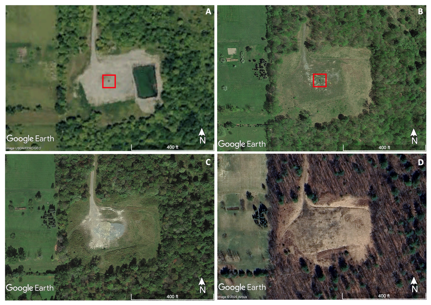
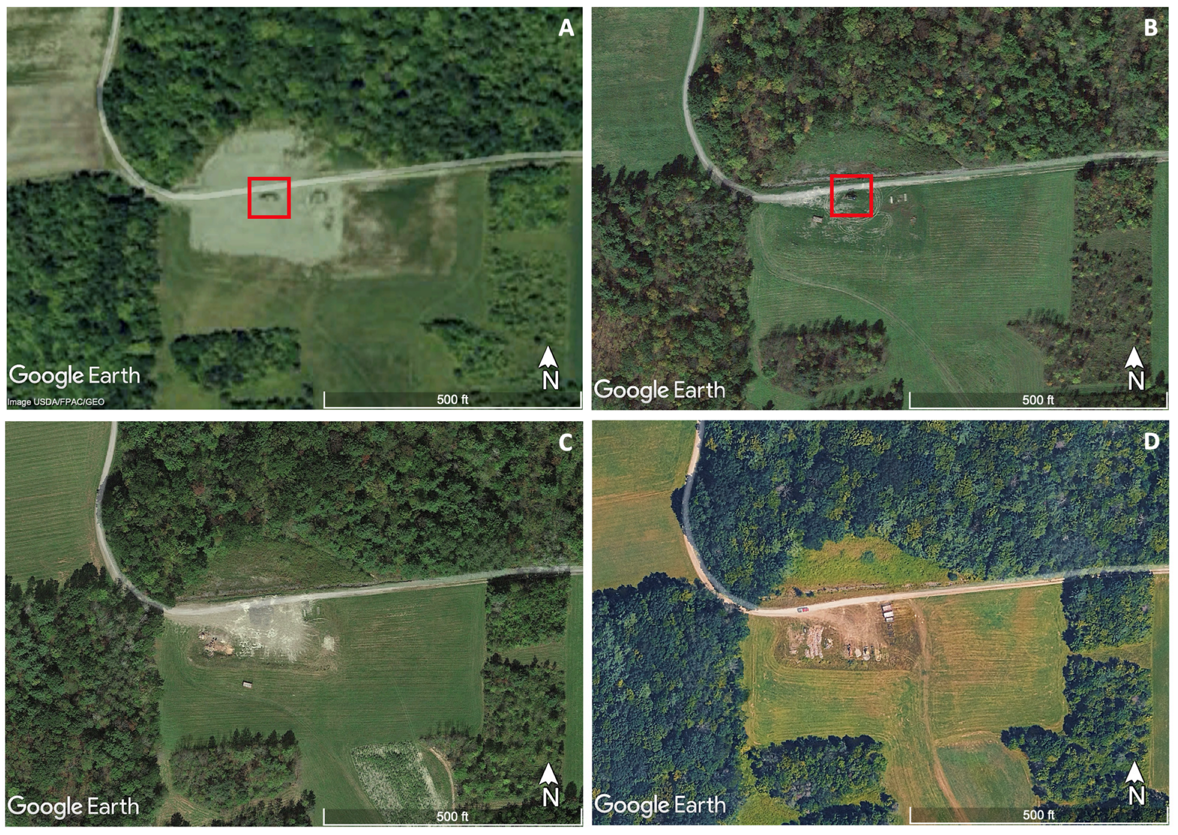
Surveys were conducted at the Butkowsky 1-A well site near Binghamton, New York (Figure 1). Completed in 2005 as a gas wildcat well at 10,137 ft (3090 m), Butkowsky 1-A was documented as plugged and abandoned in 2017 by Chesapeake Appalachia, LLC in the NYS DEC oil and gas well database [84]. Historical satellite imagery of the wellhead from 2006 to 2015 pinpoints the location of the wellhead after completion (Figure 1A,B). In 2017, satellite imagery confirms that the wellhead was removed during the plugging and abandonment process (Figure 1C). Since abandonment, the area has been reclaimed by natural vegetation that has covered surface evidence of the well’s location in the open field (Figure 1D). During the data collection process, reconnaissance surveys were conducted at a nearby well site of the documented Beagell 2-B plugged and abandoned well. Similarly to the Butkowsky 1-A well site, the absence of a wellhead has removed clues of the well’s presence and precise location. Further information on the Beagell 2-B survey site can be found in Appendix A.1.

5.2. Instrumentation Setup

Magnetic field and location data were collected using the free smartphone application, phyphox, which utilizes existing internal smartphone sensors to collect raw data that can be exported as spreadsheet files for processing and interpretation [85]. Surveyors downloaded phyphox to their personal smartphones for this study, providing an organic range of Android and iPhone models. Across 10 surveyors, the following assemblage of smartphone devices was utilized: 1 Samsung Galaxy S24+, 1 Apple iPhone 8, 3 Apple iPhone 13s, 1 Apple iPhone 13 Pro, 1 Apple iPhone 15, 2 Apple iPhone 15 Pros, and 1 Apple iPhone 16 Pro Max. The Samsung Galaxy S24+ contains an AK09918 Hall effect magnetometer sensor with a sensitivity of 0.15 µT [86]. Magnetometers inside the Apple smartphones used in this study were not provided within the available metadata, meaning the exact sensor specifications are unknown and are assumed to resemble previous iPhone teardown reports. Teardowns of previous iPhone 5 models have identified that the AK8963 Hall effect magnetometer sensor has been used within Apple iPhones with a similar sensitivity of 0.6 µT/LSB configured in 14-bit resolution and 0.15 µT/LSB in 16-bit resolution [87].
Unless otherwise specified, the standard magnetometer sampling rate for the surveys in this study was set within phyphox to match the commonly fixed rate of 1 Hz for the internal GPS sensor. This aligned sensor rate allows for the location of each magnetic data point to be recorded, increasing the accuracy of detected well magnetic anomaly locations and minimizing the amount of data processing via interpolation required. As smartphone magnetometers are sensitive to external interference [22], wearable objects such as watches, belts, and smartphone cases containing magnetic material were removed and placed outside of the survey area boundaries.

5.3. Smartphone Survey Procedure

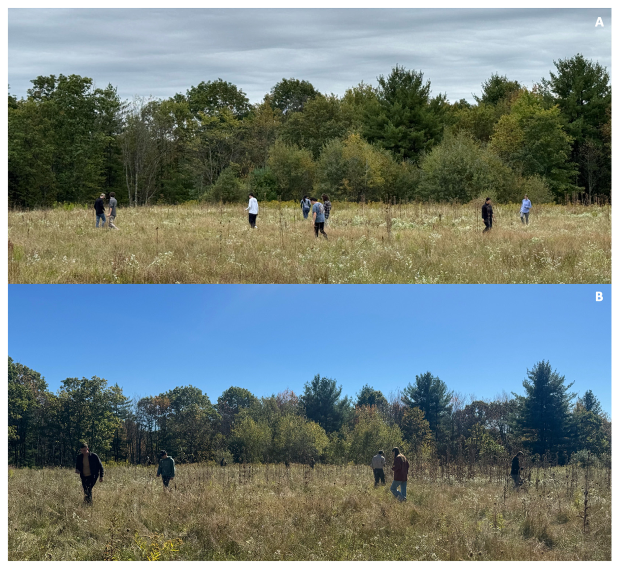
Walking surveys were conducted at the well site in 2024 and 2025 following the instrumentation setup. For all surveys in this study, smartphones were orientated parallel to the surface at a height of approximately 1 m (Figure 2). For simplicity of the survey procedure, data were collected dynamically by walking freely throughout the area. In 2024, data was collected in alternating east–west transects for 68 min over a 4800 m2 area. In October 2025, 10 surveyors collected independent data concurrently while walking freely around the grass field. These surveys varied from 29 to 56 min, with 1 of the 10 magnetometers adjusted to a sampling of 100 Hz. Afterward, a 2900 m2 area was partitioned into 10 sections, one for each surveyor. Within each of the concentrated spaces, data was simultaneously collected for 22 min. It is worth noting that one of the datasets from this cumulative survey was lost. However, as it was collected on the edge of the survey about 20 m from the well, the ability to locate the well was not impacted by this data loss.

5.4. Data Processing

Raw smartphone magnetometer and location data was analyzed to remove low-accuracy data collected during initial sensor calibrations and to interpolate the location of total magnetic field data that did not have an exact corresponding GPS measurement due to slight misalignment in sensor data collection.
Magnetometer and GPS data were cleaned to remove low-accuracy measurements taken during initial sensor calibrations at the beginning of the survey and in the presence of intermittent breaks throughout data collection. Data collected by the GPS during sensor calibrations (~0–10 s) exhibited rogue sampling frequency and extremely low accuracy (10–1100 m). Once calibrated, the GPS sampling frequency remained constant throughout the surveys. To remove inaccurate GPS measurements, data that deviated by more than 20% from the average pre-determined sampling frequency were removed. For example, a dataset collected at 1 Hz was cleaned by removing data that was collected less than 0.8 s or more than 1.2 s from the previous reading.
Due to the magnetometer and GPS sensors independently collecting concurrent data, their sampling frequencies can marginally differ for surveys collected at 1 Hz. For magnetometer data collected at a different sampling frequency than the GPS, many points do not have a corresponding location due to the fixed GPS sampling frequency of 1 Hz. To calculate the exact location of magnetic field datapoints (lati, loni) that do not have corresponding GPS positioning measured by the smartphone’s GPS, linear interpolation was performed using the timestamp (t0loc, t1loc), latitude (lat0loc, lat1loc), and longitude (lon0loc, lon1loc) of the GPS data collected directly before and after the magnetic sample at time tmag using the following equations:
interpolation   fraction   ( µ )   =   ( t mag − t loc 0 ) ( t loc 1 − t loc 0 )
lat i = lat loc 0 × 1 − µ + lat loc 1 × µ
lon i =   lon loc 0   ×   1 − µ + lon loc 1 × µ
Following data cleaning and interpolation, the total magnetic field intensity (BT) was calculated from the magnitudes of the individual magnetic field directions (BX, BY, BZ) measured by the smartphone’s magnetometer sensor using the following equation:
B T   = B X 2   +   B Y 2   +   B Z 2
Earth’s regional total magnetic field at the survey location was estimated from the International Geomagnetic Reference Field (IGRF) value at the survey location and times. Values of 51.956 µT and 51.8406 µT for the 2024 and 2025 surveys [88], respectively, were subtracted from BT measurements to calculate the residual magnetic intensity of local magnetic anomalies throughout the survey area. No additional filtering was performed as background noise was determined to be minimal and did not impact the ability to locate the well.
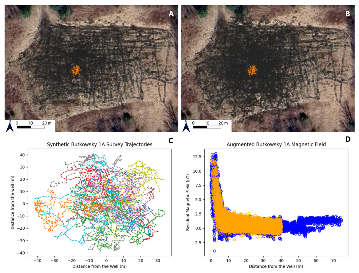
To evaluate the radius of magnetic anomalies detected by the smartphones, the distance of data points from the well was calculated by converting raw location decimal coordinates into UTM distance meters using the utm python package [89]. Using AI diffusion-based generative modeling, magnetic data points and synthetic survey trajectories were generated within a 40 m radius of the well’s coordinates to aid in locating wells using Variational Mode Decomposition (VMD) and Density-Based Spatial Clustering of Applications with Noise (DBSCAN), followed by a separate explainability step to interpret point-to-cluster assignments [90].
The diffusion-based augmentation was treated as a robustness and data-density step rather than as an independent source of ground truth. The generated samples were concentrated in the near-well response zone and then combined with measured smartphone data to form synthetic walking trajectories within the 40 m analysis radius. Quantitative validation compared the resulting clustered anomaly outputs with the documented well position using the centroid-to-well distance, uncertainty radius, and whether a trajectory produced at least one clustered anomaly after thresholding. In the companion technical analysis, the processed field-survey set contained 10 real surveys and 27,912 cleaned points; all 10 surveys produced at least one clustered anomaly. The AI-enhanced simulated set contained 50 synthetic trajectories and 96,222 points; 35 trajectories produced at least one clustered anomaly and were retained for centroid-distance and uncertainty analysis.
The VMD was used as a signal-separation step to isolate anomaly-sensitive magnetic components from slower background variation and high-frequency noise before spatial clustering. Each survey was decomposed into 10 modes, and then retained modes were selected with rule-based screening and summarized using sliding-window root mean square scoring with robust median and median absolute deviation normalization. The tested parameter ranges included physical window lengths of 5, 8, 10, 12, and 15 m; step ratios of 0.25 and 0.5; and anomaly threshold factors of 2, 3, 4, 5, and 6. These parameters control the tradeoff between sensitivity and stability: shorter windows and lower thresholds can detect sharper localized changes but may increase isolated or fragmented detections, whereas longer windows and higher thresholds smooth the response but may reduce spatial precision near the well. The resulting high-scoring window centers were grouped using DBSCAN. In the DBSCAN method, the neighborhood radius controls whether nearby anomaly responses are merged into one candidate zone or split into smaller clusters, while the minimum-sample setting prevents isolated points from being interpreted as candidate well locations. A sensitivity sweep over neighborhood radius values of 1.5 to 4.0 m and minimum-sample values of 3 to 7 supported the use of a 4.0 m radius and five minimum samples for this site, because smaller radii fragmented the same well-related response into multiple clusters while the selected setting preserved compact candidate zones around the anomaly. These settings are therefore interpreted as site-specific choices for stable clustering, not universal parameters for all future survey sites.

6. Results and Discussion

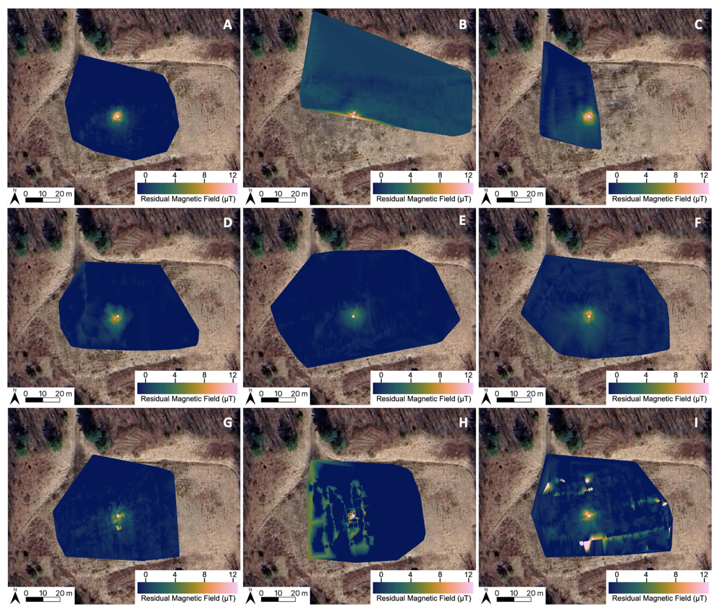
The Butkowsky 1-A well was located by the 11 smartphone magnetometers in the 2024 and 2025 proof-of-concept surveys, providing a 100% success rate across 11 surveys (Figure 3, Figure 4 and Figure 5). The strong magnetic monopole anomaly with a radius of ~2.5 m (Figure 3, Figure 4 and Figure 5) aligns with the location of magnetic anomalies from previous aeromagnetic surveys of the well [42] and NYS DEC oil and gas well documentation [84]. Measuring the distance between the maximum measured signal and the well’s documented location, the 11 smartphone surveys produced a median error of 2.05 m. An extreme outlier of 8.78 m (Figure 4G and Figure 5G) resulted in an average error of 2.5 m and a root mean square error (RMSE) of 3.34 m. GPS positioning demonstrated average accuracies of 5.3 m (horizontal) and 4.3 m (vertical), with median accuracies of 5.0 m (horizontal) and 4.6 m (vertical).
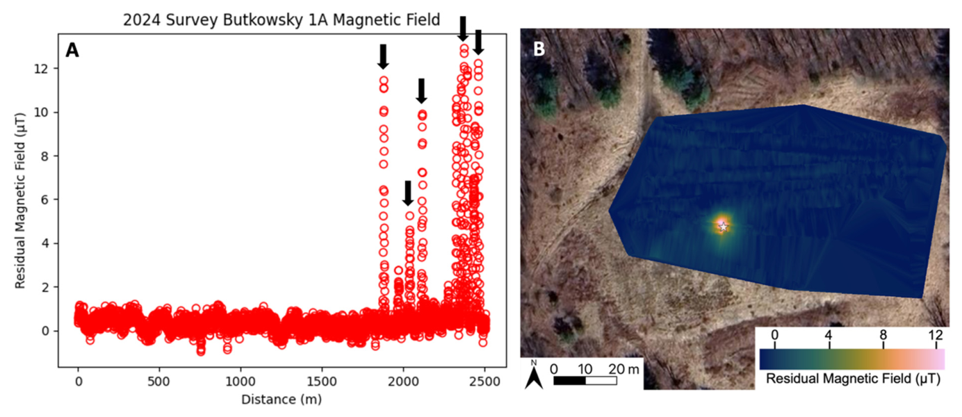
The residual magnetic map for the 2024 survey (Figure 3) shows the magnetic anomaly is 12.9 µT greater than the background magnetic field of 51.956 µT, representing the well. The background magnetic signal appears noise-free, resulting in a clear delineation of the well’s location.
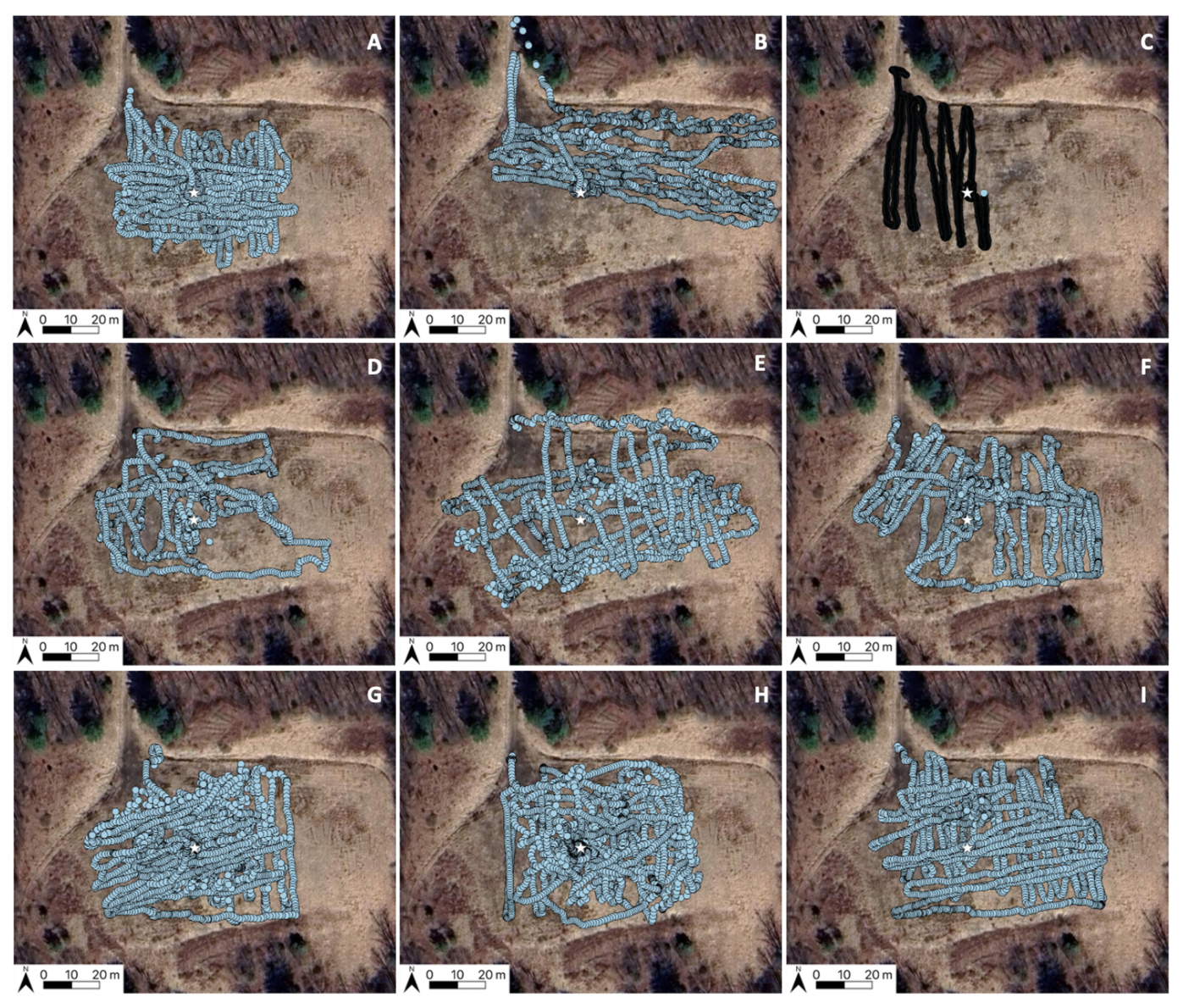
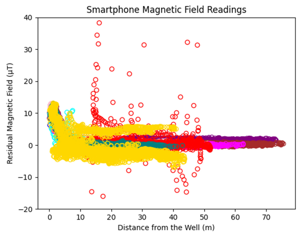
The residual magnetic maps for the nine individual surveys in 2025 are shown in Figure 4. The location of the well is resolved in each survey with magnetic anomalies ranging from 5.58 µT to 13.14 µT above the background magnetic field of 51.8406 µT (Figure 5). The range in magnetic anomaly values is partly the result of the surveyor’s data collection path. Most surveys detected an anomaly with a maximum of 12–13 µT above the background within 5–10 m of the well (Figure 5 and Figure 6), while surveys with sparser data points in the vicinity of the well resulted in a weaker magnetic signal (e.g., Figure 4E and Figure 5E).
Magnetic signal noise differs across all datasets, which is likely attributed to the number of irregularities in the survey paths, the density of data collection, and surveyors’ operational discrepancies. Surveys with denser data points and straight survey paths generally exhibited clean results of a symmetrical magnetic monopole, which is especially seen in Figure 5A. Exceptions to this could be attributed to decreased accuracy of magnetic sensor readings, as is apparent in the case of Figure 5G, whose survey exhibited a locating error of 8.78 m. This may be impacted by frequent movement in alternating directions, as well as environmental conditions such as cloud coverage impacting the smartphone’s GPS, signal interference due to proximity to smartphones of fellow surveyors or personal magnetic objects that were not removed.
The 65,536-row limit of .xls Excel-formatted files was reached 6 min and 34 s into the 29 min and 37 s survey with the magnetometer set to 100 Hz, resulting in a loss of most of the magnetic field data. The well was detected within the partial dataset (Figure 4C and Figure 5C), providing insight into the smartphone’s ability to detect wells at high resolutions. For future surveys, exporting data from phyphox as a delimited text file will resolve this issue.
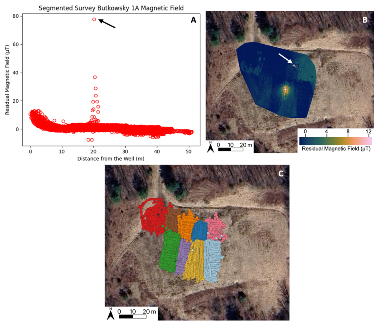
Figure 7 shows the results of the segmented magnetic data collected by nine surveyors (five segments on the top and four segments on the bottom of the partitioned area). The 12.9 µT monopole signature of the well is clearly delineated against the background. Each segment displays a unique range of noise, which is likely the result of the path taken by the surveyor. Surveys with more irregular travel paths collected noisier data, while those with more structure produced smoother results. Overall, the dense data collected produced a magnetic map that generally appeared noise-free. However, sharp magnetic interference is present in a segment in the northwest portion of the segmented survey (Figure 7), which resembles the noise visible in Figure 5I, the individual survey. These two datasets were collected by the same surveyor, which suggests that there was potentially a personal magnetic object left on the surveyor during data collection. Although background noise did not hinder the ability to locate the buried well, excess background noise due to repeated interference of magnetic objects near the phone could result in illegible data in extreme cases.
The relatively low sensitivity of smartphone magnetometers did not hinder their ability to locate the well across the 11 unique surveys conducted in this study (Figure 6). As with professional instruments, dense and symmetrical data provided clearer results. However, the consistent detection of the buried steel casing at the well’s documented location across dense and sparse surveys indicates that this is not necessary to resolve the prominent magnetic signature of steel-cased wells with smartphones. Although the positive magnetic signal is consistently aligned with well documentation, the average GPS sensor horizontal accuracy of 5.3 m and median error of 2.05 m within the noise-free environment indicates that validation using professional instrumentation is likely necessary to ensure accurate detection of undocumented wells for applications where significant noise may be present (e.g., urban environments, dense vegetation).
To assess the generalizability potential of the survey method, results from reconnaissance smartphone surveys at a second well site were analyzed. The smartphones in this survey provided similar results to the Butkowsky 1-A smartphone surveys, consistently locating the Beagell 2-B well at an average magnitude of 7.8 µT with an average distance error of 4.97 m and RMSE of 4.98 m. Detailed residual magnetic maps and smartphone performance metrics are provided within Appendix A (Figure A2).
The diffusion-based generative modeling produced realistic magnetic data across synthetic survey trajectories to increase the density of smartphone magnetic data (Figure 8) [90]. This AI approach has the potential to aid in enhancing the magnetic signal detected from sparse datasets into clear magnetic signals. Doing so, data collected in areas that are difficult for human traversal or for surveyors that marginally detected a well’s signal (e.g., Figure 4E and Figure 5E) will be sufficient to accurately pinpoint a well without requiring additional data collection.
The processed field-survey set produced nearest detected centroid distances of 0.91 to 3.86 m from the known well, with a median field offset of 1.82 m, and the support-screened minimum-uncertainty neighborhood matched the nearest centroid in 9 of 10 field surveys. For the 50 AI-enhanced simulated trajectories, 35 produced at least one clustered anomaly after thresholding. In these 35 trajectories, selected centroids were 0.03 to 0.67 m from the known well, with a median distance of 0.27 m, and uncertainty radii ranged from 0.19 to 0.71 m, with a median of 0.49 m. These results demonstrate that synthetic data generation improved the near-well spatial density and produced stable candidate well-position estimates under sparse-trajectory conditions. However, because the simulated trajectories were intentionally concentrated near the strongest response zone, they are interpreted as robustness and sensitivity evidence rather than independent field validation.
The magnetometry method is limited to detecting wells whose steel casing remains in the ground. Wells that have had their steel casing removed during abandonment or were cased with a different material (e.g., wood) are therefore undetectable by smartphone magnetometers. Given this limitation, smartphone magnetometers should be used alongside a complementary well detection method that does not rely on casing material for well identification (e.g., imagery and LiDAR) if applied nationwide. Further, as the steel casing of a well undergoes corrosion, its magnetic signature becomes increasingly weaker [28,29]. In instances of extreme long-term corrosion or partially removed steel casing, it may be challenging for smartphones to isolate a strong anomaly that is easily identifiable as a steel-cased well. Similarly, well casings buried deep into the subsurface have the potential to produce a diminished signal for sensors at the surface. Unlike the documented well detected in this study, undocumented wells surrounded by urban infrastructure have a higher likelihood of experiencing magnetic interference [43,47]. As a result, future nationwide applications should consider conducting a combination of smartphone and professional magnetic surveys within high-interference areas to ensure that wells of varying ages, corrosion, well depths, and proximity to nearby magnetic objects are detected accurately. Potential avenues may include crowd-sourced smartphone data collected passively during outdoor recreation in public spaces (e.g., hiking, walking) alongside active surveys for those seeking to reduce financial cost to pinpoint areas of interest for further investigations.
The portability of smartphone magnetometers allowed for dense data collection, which resulted in a more concentrated and smaller-diameter magnetic anomaly than previous UAV magnetometry surveys at the well site with wider line spacing [42]. As the nature of the monopole magnetic anomaly centers the maximum signal directly above the buried steel casing, this method has the potential to provide a more accurate prediction of the well’s true location than broad anomalies detected by aerial magnetometry, resistivity plumes from groundwater contamination, and remnants scattered around the drilling site seen in visual data.
This proof-of-concept study primarily focused on verifying the performance of smartphone magnetometers in varying survey patterns. Further, the replication of well location at the secondary survey site (Appendix A) demonstrates generalizability of the smartphone magnetometry method across multiple well sites. The reproducibility of well location results during these rapid surveys demonstrates the ability of smartphones to quickly detect the well’s strong magnetic signal within roughly 2–5 m of the steel casing’s burial location. While both surveys demonstrated a generally consistent well location error, the relatively high RMSE (3.34 m for Butkowsky 1-A and 4.98 m for Beagell 2-B) indicates that the presence of high interference could impact the ability to correctly concentrate the location of potential undocumented wells. Therefore, to investigate the variations in smartphone magnetometry results across well types and status, future work should apply the unsupervised smartphone survey method demonstrated in this study to well sites within different settings. Specifically, future work should analyze the performance of smartphone and professional magnetometers when significant magnetic and GPS signal noise is present to ensure that smartphone magnetometers can detect and isolate the signal from undocumented wells in urban environments, in the presence of nearby metallic infrastructure (e.g., vehicles, leftover drilling debris, overlain structures, powerlines, underground pipes), and busy natural environments (e.g., dense vegetation, severe weather).
Given the low cost and simplicity of instrument initialization compared to professional geophysical equipment, smartphone magnetometry can directly target steel-cased wells with minimal financial burden and technical expertise. The AI-based approach for generating realistic synthetic data surrounding the well provides a promising aid to locating wells with a variety of datasets, enabling the identification and location of undocumented steel-cased wells using sparse datasets collected with smartphones at marginal cost and physical effort compared to professional methodologies.

7. Conclusions

The smartphones in this study located an abandoned gas well when walking within 2.5 m of the well’s buried steel casing with a median error of 2.05 m. Despite a lower sensitivity and horizontal accuracy than professional magnetometers, the smartphones detected the well without impeding signal noise. As this persisted across unsupervised survey patterns of various data density, the results of this proof-of-concept study suggest locating steel-cased wells is not dependent on surveyors with proficiency in field surveying techniques. This expands the pool of magnetic surveyors to any person who can travel throughout an area while holding a smartphone, reducing the necessity to rely on professional geophysicists for reconnaissance surveying. While UAV systems have allowed for professional surveyors to rapidly collect data throughout an area, ground-based smartphone magnetometry has the potential to provide an avenue for amateur and professional surveyors to collaborate in a large-scale effort for orphaned well documentation nationwide. Furthermore, diffusion AI modeling showed a promising approach to improve well locating by enhancing sparse datasets with generated realistic near-well magnetic data, paving the way for automated well detection with AI and machine learning.
Using smartphone magnetometry, any person with access to a smartphone and the ability to travel throughout an area can assist in locating steel-cased wells. For owners of private land, students and researchers with limited funding, and consultants looking to improve financial and survey efficiency, smartphones open the door for simple, affordable, and low-effort magnetic surveying. This enhanced pool of potential surveyors could enable faster identification and remediation of the remaining millions of orphaned wells across the U.S. through crowd-sourced data collection. This approach can potentially help mitigate groundwater and soil contamination and reduce methane emissions, contributing to improved public health and reduced greenhouse gas emissions with less financial burden.

Author Contributions

Conceptualization, C.S., S.N., S.K. and S.S.; methodology, C.S., S.N., S.K. and S.S.; validation, C.S., S.N., S.K. and S.S.; formal analysis, C.S. and S.N.; investigation, C.S., S.N., S.K. and S.S.; resources, S.K. and S.S.; data curation, C.S. and S.N.; writing—original draft preparation, C.S. and S.S.; writing—review and editing, C.S., S.N., S.K. and S.S.; visualization, C.S. and S.N.; supervision, S.K. and S.S.; project administration, S.K. and S.S.; funding acquisition, S.K. and S.S. All authors have read and agreed to the published version of the manuscript.

Funding

This research received no external funding.

Institutional Review Board Statement

Not applicable.

Informed Consent Statement

Not applicable.

Data Availability Statement

The original data presented in this study are openly available at https://doi.org/10.5281/zenodo.20837070.

Acknowledgments

We extend our gratitude to Tricia and Michael Jewson for granting us access to their property to conduct our research. Thank you to Anna Brown, Jillian Martinek, Seth McKee, Alyssa Mercado, Aidan Okeefe, Jacob Tennant, Lea Viegl, and Kayla Yoder for assisting in data collection and providing data used in this study. Thank you to Binghamton University for supporting this project through the Transdisciplinary Areas of Excellence program.

Conflicts of Interest

The authors declare no conflicts of interest.

Abbreviations

The following abbreviations are used in this manuscript:
AIArtificial Intelligence.
UAVUnmanned Aerial Vehicle.
U.S. EPAUnited States Environmental Protection Agency.
USGSUnited States Geological Survey.
GPSGlobal Positioning System.
LiDARLight Detection & Ranging.
IIJAInfrastructure Investment and Jobs Act.
IGRFInternational Geomagnetic Reference Field.
RMSERoot Mean Square Error.
VMDVariational Mode Decomposition.
DBSCANDensity-Based Spatial Clustering of Applications with Noise.

Appendix A

Appendix A.1. Beagell 2-B Wellsite

Surveys were conducted at Beagell 2-B at a well site near the Butkowsky 1-A site. Beagell 2-B is a dry wildcat well completed in 2008 at 4800 ft (1463 m) just off a dirt road, then documented as plugged and abandoned in 2017 by Chesapeake Appalachia, LLC in the NYS DEC oil and gas well database [84]. Historical satellite imagery from 2009 to 2011 confirms the presence of a wellhead after completion (Figure A1A,B) and removal of the wellhead above the surface after plugging and abandonment (Figure A1C). The well site currently contains a flattened area off the road, with miscellaneous debris scattered nearby (Figure A1D). Walking scout surveys at the Beagell 2-B well site were conducted in 2025 over a 12 min period by three individual surveyors over the roughly 800 m2 area, all utilizing an Apple iPhone 15 Pro.
Figure A1. Historical Google Earth satellite imagery showing temporal evolution of the Beagell 2-B well site. Wellhead is outlined in red when visible in imagery before plugging and abandonment, (A) after well completion (2009), (B) prior to well abandonment (2011), (C) after well abandonment (2017), and (D) after natural reclamation (2026).
Ndt 04 00022 g0a1

Appendix A.2. Beagell 2-B Survey Results

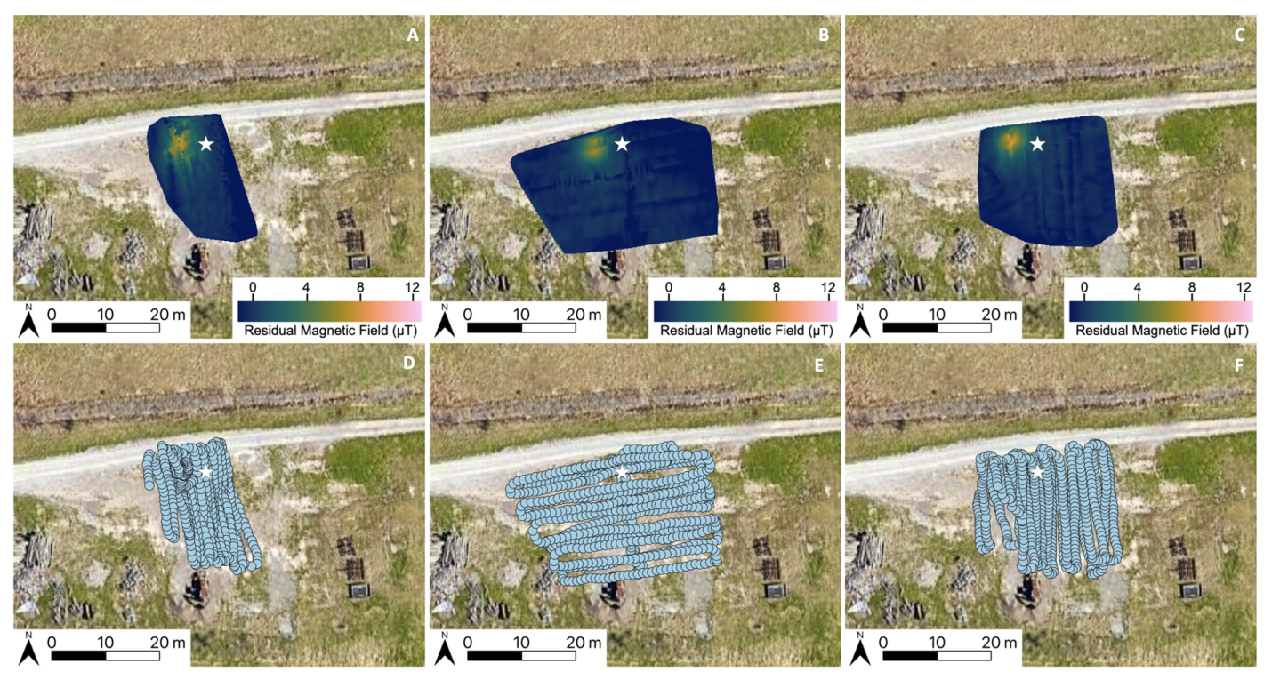
The Beagell 2-B well was located by the three smartphone surveys conducted over a 12 min period (Figure A2). The brief smartphone surveys (Appendix A.2) were conducted throughout the unpaved area off the road where plugging and abandonment took place, acting as a reconnaissance survey to confirm the presence of the documented well. After removing the IGRF value of 51.88 µT, the resulting magnetic maps reveal the average 7.8 µT residual signal from the Beagell 2-B well (Figure A2A–C). The smartphones consistently located the well at an average distance of 4.97 m (median 4.83 m) from its documented location, resulting in an RMSE of 4.98 m.
Despite the presence of nearby surface debris (as seen in satellite imagery in Figure A1 and Figure A2), the smartphones produced results that lacked background noise against the high-magnitude signal from the well’s steel casing (Figure A2A–C).
Figure A2. Smartphone survey results of the 3 individual 2025 Beagell 2-B surveys of the residual magnetic field readings (A–C) and data points collected along their respective survey paths represented by blue circles (D–F). Stars represent the documented location of the well. Data collection occurred over a 12 min period, simulating rapid data collection in real-world applications. The 3 surveys produced a strong magnetic monopole anomaly that stands out against a noise-free background.
Ndt 04 00022 g0a2

References

  1. National Petroleum Council. Working Document of the NPC North American Resource Development Study Made PLUGGING AND ABANDONMENT OF OIL AND GAS WELLS. 2011. Available online: https://www.npc.org/Prudent_Development-Topic_Papers/2-25_Well_Plugging_and_Abandonment_Paper.pdf (accessed on 20 June 2025).
  2. Kang, M.; Kanno, C.M.; Reid, M.C.; Zhang, X.; Mauzerall, D.L.; Celia, M.A.; Chen, Y.; Onstott, T.C. Direct measurements of methane emissions from abandoned oil and gas wells in Pennsylvania. Proc. Natl. Acad. Sci. USA 2014, 111, 18173–18177. [Google Scholar] [CrossRef] [Scilit] [PubMed]
  3. Boutot, J.; Peltz, A.S.; McVay, R.; Kang, M. Documented Orphaned Oil and Gas Wells Across the United States. Environ. Sci. Technol. 2022, 56, 14228–14236. [Google Scholar] [CrossRef] [Scilit] [PubMed]
  4. Townsend-Small, A.; Ferrara, T.W.; Lyon, D.R.; Fries, A.E.; Lamb, B.K. Emissions of coalbed and natural gas methane from abandoned oil and gas wells in the United States. Geophys. Res. Lett. 2016, 43, 2283–2290. [Google Scholar] [CrossRef] [Scilit]
  5. Yahya, S.; Kee, K.E.; Puad, M.J.M.; Ismail, M.C. Evaluation on steel corrosion in water-based drilling fluids: Inhibitors and scale involvement. J. Pet. Sci. Eng. 2022, 211, 110127. [Google Scholar] [CrossRef] [Scilit]
  6. Pennsylvania Department of Environmental Protection (PA DEP). Shapiro Administration Plugs Orphan Well That Contaminated Family’s Water. Pa.gov. 2025. Available online: https://www.pa.gov/agencies/dep/newsroom/shapiro-administration-plugs-orphan-well-that-contaminated-famil.html (accessed on 24 March 2026).
  7. Kang, M.; Boutot, J.; McVay, R.; Roberts, K.A.; Jasechko, S.; Perrone, D.; Wen, T.; Lackey, G.; Raimi, D.; DiGiulio, D.C.; et al. Environmental risks and opportunities of orphaned oil and gas wells in the United States. Environ. Res. Lett. 2023, 18, 074012. [Google Scholar] [CrossRef] [Scilit]
  8. U.S. EPA. Inventory of U.S. Greenhouse Gas Emissions and Sinks: 1990–2022. 8 February 2024. Available online: https://www.epa.gov/ghgemissions/inventory-us-greenhouse-gas-emissions-and-sinks-1990-2022 (accessed on 24 February 2026).
  9. Lebel, E.D.; Lu, H.S.; Vielstädte, L.; Kang, M.; Banner, P.; Fischer, M.L.; Jackson, R.B. Methane Emissions from Abandoned Oil and Gas Wells in California. Environ. Sci. Technol. 2020, 54, 14617–14626. [Google Scholar] [CrossRef] [Scilit] [PubMed]
  10. Riddick, S.N.; Mauzerall, D.L.; Celia, M.A.; Kang, M.; Bressler, K.; Chu, C.; Gum, C.D. Measuring methane emissions from abandoned and active oil and gas wells in West Virginia. Sci. Total Environ. 2019, 651, 1849–1856. [Google Scholar] [CrossRef] [Scilit] [PubMed]
  11. Riddick, S.N.; Mbua, M.; Santos, A.; Emerson, E.W.; Cheptonui, F.; Houlihan, C.; Hodshire, A.L.; Anand, A.; Hartzell, W.; Zimmerle, D.J. Methane emissions from abandoned oil and gas wells in Colorado. Sci. Total Environ. 2024, 922, 170990. [Google Scholar] [CrossRef] [Scilit] [PubMed]
  12. Pekney, N.J.; Diehl, J.R.; Ruehl, D.; Sams, J.; Veloski, G.; Patel, A.; Schmidt, C.; Card, T. Measurement of methane emissions from abandoned oil and gas wells in Hillman State Park, Pennsylvania. Carbon Manag. 2018, 9, 165–175. [Google Scholar] [CrossRef] [Scilit]
  13. National Academies of Sciences, Engineering, and Medicine. Practices and Standards for Plugging Orphaned and Abandoned Hydrocarbon Wells. In National Academies Press EBooks; The National Academies Press: Washington, DC, USA, 2025. [Google Scholar] [CrossRef] [Scilit] [PubMed]
  14. Woda, J.; Haase, K.B.; Gianoutsos, N.J.; Jahn, K.; Gutchess, K. A geospatial analysis of water-quality threats from orphan wells in principal and secondary aquifers of the United States. Sci. Total Environ. 2025, 976, 179246. [Google Scholar] [CrossRef] [Scilit] [PubMed]
  15. Orphaned Well Program Office (OWPO). Orphaned Wells Program Annual Report to Congress for Fiscal Year 2025. November 2025. Available online: https://www.doi.gov/orphanedwells (accessed on 24 March 2026).
  16. Raimi, D.; Krupnick, A.J.; Shah, J.-S.; Thompson, A. Decommissioning Orphaned and Abandoned Oil and Gas Wells: New Estimates and Cost Drivers. Environ. Sci. Technol. 2021, 55, 10224–10230. [Google Scholar] [CrossRef] [Scilit] [PubMed]
  17. Jordan, P.W.; Hare, J.L. Locating Abandoned Wells: A Comprehensive Manual of Methods and Resources. Solution Mining Research Institute. 2002. Available online: https://legacy.zonge.com/locating-abandoned-wells-a-comprehensive-manual-of-methods-and-resources/ (accessed on 26 February 2026).
  18. Frischknecht, F.C.; Grette, R.; Raab, P.V.; Meredith, J. Location of Abandoned Wells by Magnetic Surveys; Acquisition and Interpretation of Aeromagnetic Data for Five Test Areas; United States Geological Survey: Reston, VA, USA, 1985. [CrossRef] [Scilit]
  19. Aller, L. Methods for Determining the Location of Abandoned Wells; Robert, S., Ed.; Kerr Environmental Research Laboratory, Office of Research and Development, U.S. Environmental Protection Agency: Ada, OK, USA, 1984.
  20. O’Malley, D.; Delorey, A.A.; Guiltinan, E.J.; Ma, Z.; Kadeethum, T.; Lackey, G.; Lee, J.; Santos, J.E.; Follansbee, E.; Nair, M.C.; et al. Unlocking Solutions: Innovative Approaches to Identifying and Mitigating the Environmental Impacts of Undocumented Orphan Wells in the United States. Environ. Sci. Technol. 2024, 58, 19584–19594. [Google Scholar] [CrossRef] [Scilit] [PubMed]
  21. Eraky, M.M.; Abdelaal, G.Z.; El-Haddad, A.E. Detection of Depth and Location of Subsurface Utilities Using Smart Phone Magnetic Application: A Case Study at Assiut University, Egypt. Assiut Univ. J. Multidiscip. Sci. Res. 2022, 1, 175–190. [Google Scholar] [CrossRef] [Scilit]
  22. Campbell, N.; Atekwana, E.A.; Mathews, A.J.; Ismail, A. Geophysical applications of magnetic sensors in smartphones. Lead. Edge 2020, 39, 312–317. [Google Scholar] [CrossRef] [Scilit]
  23. Saneiyan, S.; Mansourian, D. Locating undocumented orphaned oil and gas wells with smartphones. J. Appl. Geophys. 2023, 219, 105224. [Google Scholar] [CrossRef] [Scilit]
  24. Saint-Vincent, P.M.B.; Sams, J.I., III; Hammack, R.W.; Veloski, G.A.; Pekney, N.J. Identifying Abandoned Well Sites Using Database Records and Aeromagnetic Surveys. Environ. Sci. Technol. 2020, 54, 8300–8309. [Google Scholar] [CrossRef] [Scilit] [PubMed]
  25. Hammack, R.W.; Veloski, G.A.; Hodges, D.G.; White, C.M. Methods for Finding Legacy Wells in Large Areas; NETL-TRS-6-2016; EPAct Technical Report Series; U.S. Department of Energy, National Energy Technology Laboratory: Morgantown, WV, USA, 2016; p. 28.
  26. Kaminski, V.; Hammack, R.W.; Harbert, W.; Veloski, G.A.; Sams, J.; Hodges, D.G. Geophysical helicopter-based magnetic methods for locating wells. Geophysics 2018, 83, B269–B279. [Google Scholar] [CrossRef] [Scilit]
  27. Saint-Vincent, P.M.B.; Sams, J.I., III; Mundia-Howe, M.; Reeder, M.D.; Veloski, G.A.; Pekney, N.J. Historic and modern approaches for discovery of abandoned wells for methane emissions mitigation in Oil Creek State Park, Pennsylvania. J. Environ. Manag. 2021, 280, 111856. [Google Scholar] [CrossRef] [Scilit] [PubMed]
  28. Schifano, V.; Marquis, G.; Matthey, P.-D.; Luling, M.G.; Bennani, H.K.; Kassir, L.; Kassir, M. Magnetic Induction Sensing of Corrosion on Steel Pipes: Feasibility, Instrument Design and First Test Results. Sensors 2026, 26, 1630. [Google Scholar] [CrossRef] [Scilit] [PubMed]
  29. Veloski, G.; Hammack, R.; Sams, J., III. Results From an Aeromagnetic Survey to Detect Steel-Cased Wells at a Marcellus Shale Well Site in Washington County, Pennsylvania; DOE.NETL-2025.4891. NETL Technical Report Series; U.S. Department of Energy, National Energy Technology Laboratory: Morgantown, WV, USA, 2024. [CrossRef] [Scilit]
  30. DiGiulio, D.C.; Rossi, R.J.; Lebel, E.D.; Bilsback, K.R.; Michanowicz, D.R.; Shonkoff, S.B.C. Chemical Characterization of Natural Gas Leaking from Abandoned Oil and Gas Wells in Western Pennsylvania. ACS Omega 2023, 8, 19443–19454. [Google Scholar] [CrossRef] [Scilit] [PubMed]
  31. Heagle, D.J.; Sealey, R. The Implications of Ontario’s Historical Oil and Gas Drilling and Abandonment Practices for Abandoning Orphan and Legacy Wells. Geosci. Can. 2023, 50, 277–294. [Google Scholar] [CrossRef] [Scilit]
  32. Meehan, D.N.; Liu, M.; Kang, M.; Peltz, A.S. Environmental Issues with Orphaned Wells. In Proceedings of the SPE Annual Technical Conference and Exhibition, Houston, TX, USA, 20–22 October 2025. [Google Scholar] [CrossRef] [Scilit]
  33. Atekwana, E.A.; Atekwana, E.A.; Rowe, R.S.; Werkema, D.D., Jr.; Legall, F.D. The relationship of total dissolved solids measurements to bulk electrical conductivity in an aquifer contaminated with hydrocarbon. J. Appl. Geophys. 2004, 56, 281–294. [Google Scholar] [CrossRef] [Scilit]
  34. Rusydi, A.F. Correlation between conductivity and total dissolved solid in various type of water: A review. IOP Conf. Ser. Earth Environ. Sci. 2018, 118, 012019. [Google Scholar] [CrossRef] [Scilit]
  35. Mustofa, M.B.; Fauzi, U.; Warsa, W.; Latief, F.D.E. The effect of brine spatial distribution on electrical resistivity during imbibition processes in unconsolidated sands. J. Appl. Geophys. 2021, 194, 104441. [Google Scholar] [CrossRef] [Scilit]
  36. Adeoti, L.; Chibuzor Anukwu, G.; Saheed Ademoye, A.; Taye Adegbite, J.; Adeogun, O.; Olutayo Adigun, E. Assessment of Hydrocarbon Pollution in Groundwater Using Electrical Resistivity Method. Curr. Appl. Sci. Technol. 2022, 23, 18. [Google Scholar] [CrossRef] [Scilit]
  37. Alao, J.O.; Balarabe, B.; Ayejoto, D.A.; Abubakar, F.; Otorkpa, O.J.; Eze, S.U. Evaluation of hydrocarbon and co-contaminants in groundwater and associated public health risks using electrical resistivity and hydrochemical data. Water Resour. Ind. 2025, 34, 100319. [Google Scholar] [CrossRef] [Scilit]
  38. Uchegbulam, O.; Ayolabi, E.A. Application of Electrical Resistivity Imaging in Investigating Groundwater Pollution in Sapele Area, Nigeria. J. Water Resour. Prot. 2014, 6, 1369–1379. [Google Scholar] [CrossRef]
  39. Martinho, E. Electrical Resistivity and Induced Polarization Methods for Environmental Investigations: An Overview. Water Air Soil Pollut. 2023, 234, 215. [Google Scholar] [CrossRef] [Scilit]
  40. Eze, S.U.; Ogagarue, D.O.; Nnorom, S.L.; Osung, W.E.; Ibitoye, T.A. Integrated geophysical and geochemical methods for environmental assessment of subsurface hydrocarbon contamination. Environ. Monit. Assess. 2021, 193, 451. [Google Scholar] [CrossRef] [Scilit] [PubMed]
  41. Saribudak, M.; Rucker, D.F.; Haas, A. Electrical Resistivity Imaging near Abandoned Steel Oil Wells: Five Case Studies, USA. J. Environ. Eng. Geophys. 2020, 25, 545–556. [Google Scholar] [CrossRef] [Scilit]
  42. Nikulin, A.; de Smet, T.S. A UAV-based magnetic survey method to detect and identify orphaned oil and gas wells. Lead. Edge 2019, 38, 447–452. [Google Scholar] [CrossRef] [Scilit]
  43. Hammack, R.; Veloski, G.; Sams, J.; Kohnke, C. Aeromagnetic surveys for the location of undocumented orphaned wells. Lead. Edge 2023, 42, 798–807. [Google Scholar] [CrossRef] [Scilit]
  44. Patton, J.A.; Davis, M.; Gowing, K.; Vickers, H. Optimum Magnetometer Transect Spacing to Locate Legacy Oil and Gas Wells: Preliminary Results. J. Ark. Acad. Sci. 2018, 72, 129–134. [Google Scholar] [CrossRef] [Scilit]
  45. Veloski, G.A.; Hammack, R.W.; Lynn, R.J. Practical Methods for Locating Abandoned Wells in Populated Areas. In Symposium on the Application of Geophysics to Engineering and Environmental Problems; National Energy Technology Laboratory: Pittsburgh, PA, USA, 2007. [Google Scholar] [CrossRef] [Scilit]
  46. Neeley, C. Utilizing A Magnometer To Locate Abandoned Oil Wells In Butler County, Kansas. Master’s Thesis, Fort Hays State University, Hays, KS, USA, 2013. [Google Scholar]
  47. Hammack, R.; Veloski, G. Methods for Finding Legacy Wells in Residential and Commercial Areas; OSTI OAI (U.S. Department of Energy Office of Scientific and Technical Information): Oak Ridge, TN, USA, 2016. [CrossRef] [Scilit] [PubMed]
  48. Borton, T.A. Use of Remote Sensing and Geophysical Techniques for Locating Abandoned Oil Wells, Wood County, Ohio. Master’s Thesis, Bowling Green State University, Bowling Green, OH, USA, 2007. [Google Scholar]
  49. Heenan, J.W.; Slater, L.; Ntarlagiannis, D.; Atekwana, E.A.; Fathepure, B.Z.; Dalvi, S.; Ross, C.; Werkema, D.D.; Atekwana, E.A. Electrical resistivity imaging for long-term autonomous monitoring of hydrocarbon degradation: Lessons from the Deepwater Horizon oil spill. Geophysics 2015, 80, B1–B11. [Google Scholar] [CrossRef] [Scilit]
  50. Ayolabi, E.A.; Folorunso, A.F.; Idem, S.S. Application of Electrical Resistivity Tomography in Mapping Subsurface Hydrocarbon Contamination. Earth Sci. Res. 2012, 2, 93. [Google Scholar] [CrossRef] [Scilit]
  51. Abdullah, W.; Aljarallah, R.; Alrashidi, A. Hydrocarbon oil-contaminated soil assessment using electrical resistivity topography. J. Eng. Res. 2014, 2, 14. [Google Scholar] [CrossRef] [Scilit]
  52. Mosleh, A.T.; Al-Obaidy, N.K. A Critical Review on Expansive Soils Including the Influence of Hydrocarbon Pollution and the Use of Electrical Resistivity to Evaluate their Properties. IOP Conf. Ser. Mater. Sci. Eng. 2021, 1076, 012097. [Google Scholar] [CrossRef] [Scilit]
  53. Amani, S.; Keshtdar, A.; Ghiassi, R. Investigation of the Effectiveness of Electrical Resistivity Tomography in Monitoring and Detecting Hydrocarbon Contamination in Sandy Soil at Various Moisture: Pilot Scale. Water Air Soil Pollut. 2024, 235, 175. [Google Scholar] [CrossRef] [Scilit]
  54. de Smet, T.S.; Nikulin, A.; Balrup, N.; Graber, N. Successful Integration of UAV Aeromagnetic Mapping with Terrestrial Methane Emissions Surveys in Orphaned Well Remediation. Remote Sens. 2023, 15, 5004. [Google Scholar] [CrossRef] [Scilit]
  55. Nikulin, A.; de Smet, T.S. UAV-based aeromagnetic surveys for orphaned well location: Emerging best practices. Lead. Edge 2023, 42, 817–823. [Google Scholar] [CrossRef] [Scilit]
  56. Rashid, K.; Speck, A.; Osedach, T.P.; Perroni, D.V.; Pomerantz, A.E. Optimized inspection of upstream oil and gas methane emissions using airborne LiDAR surveillance. Appl. Energy 2020, 275, 115327. [Google Scholar] [CrossRef] [Scilit]
  57. Wilkinson, R.; Mleczko, M.M.; Brewin, R.J.W.; Gaston, K.J.; Mueller, M.; Shutler, J.D.; Yan, X.; Anderson, K. Environmental impacts of earth observation data in the constellation and cloud computing era. Sci. Total Environ. 2024, 909, 168584. [Google Scholar] [CrossRef] [Scilit] [PubMed]
  58. Ramachandran, N.; Irvin, J.; Omara, M.; Gautam, R.; Meisenhelder, K.; Rostami, E.; Sheng, H.; Ng, A.Y.; Jackson, R.B. Deep learning for detecting and characterizing oil and gas well pads in satellite imagery. Nat. Commun. 2024, 15, 7036. [Google Scholar] [CrossRef] [Scilit] [PubMed]
  59. Seth, P.; Lin, M.; Yaw, B.D.; Boutot, J.; Kang, M.; Rolnick, D. Alberta Wells Dataset: Pinpointing Oil and Gas Wells from Satellite Imagery. arXiv 2024, arXiv:2410.09032. [Google Scholar] [CrossRef] [Scilit]
  60. Kadeethum, T.; Downs, C. Harnessing Machine Learning and Data Fusion for Accurate Undocumented Well Identification in Satellite Images. Remote Sens. 2024, 16, 2116. [Google Scholar] [CrossRef] [Scilit]
  61. Ciulla, F.; Santos, A.; Jordan, P.; Kneafsey, T.; Biraud, S.C.; Varadharajan, C. A Deep Learning Based Framework to Identify Undocumented Orphaned Oil and Gas Wells from Historical Maps: A Case Study for California and Oklahoma. Environ. Sci. Technol. 2024, 58, 22194–22203. [Google Scholar] [CrossRef] [Scilit] [PubMed]
  62. Kim, A.; Kadeethum, T.; Downs, C.; Viswanathan, H.S.; O’Malley, D. Aerial imagery dataset of lost oil wells. Sci. Data 2024, 11, 1105. [Google Scholar] [CrossRef] [Scilit] [PubMed]
  63. Dacre, C.K.; Palandro, D.A.; Oldak, A.; Ireland, A.W.; Mercer, S.M. High-resolution satellite imagery applied to monitoring revegetation of oil-sands-exploration well pads. Environ. Geosci. 2017, 24, 167–182. [Google Scholar] [CrossRef] [Scilit]
  64. Delgado-Rodríguez, O.; Shevnin, V.; Peinado-Guevara, H.; Guevara-Torres, M.L.D. Characterization of Hydrocarbon-Contaminated Sites Based on Geoelectrical Methods of Geophysical Exploration. Geophysics 2018, 85. [Google Scholar] [CrossRef] [Scilit]
  65. SAGA Geophysics, Inc. SAGA Geophysics—Geophysical Equipment Rentals. Sagageo.com. 2019. Available online: https://www.sagageo.com (accessed on 10 March 2026).
  66. K. D. Jones Instrument Corporation. Ground Resistivity Meters—K. D. Jones Instruments Corp. 24 July 2014. Available online: https://kdjonesinstruments.com/geophysical-equipment-rentals/ground-resistivity-meters/ (accessed on 10 March 2026).
  67. Aeroluxe Aviation. Earn Your Commercial Pilot License with Aeroluxe Aviation. Commercial Pilot License—Helicopter—Aeroluxe Aviation. 2025. Available online: https://www.aeroluxeaviation.com/commercial-pilot-license-helicopter/ (accessed on 10 March 2026).
  68. Helicopter Flight Instructor. Understanding How Much Helicopter Pilot Training Costs. Understanding How Much Helicopter Pilot Training Costs|HAA. 2024. Available online: https://blog.flyhaa.com/blog/helicopter-pilot-training-cost (accessed on 10 March 2026).
  69. Leopard Aviation. Pilot Training in the USA: What It Costs in 2025. Pilot Training in the USA: What It Costs in 2025. 23 June 2025. Available online: https://leopardaviation.com/pilot-training-in-the-usa-cost/ (accessed on 10 March 2026).
  70. Federal Aviation Administration (FAA). How Much Does It Cost to Get a Remote Pilot Certificate?|Federal Aviation Administration. Faa.gov. 2024. Available online: https://www.faa.gov/faq/how-much-does-it-cost-get-remote-pilot-certificate (accessed on 10 March 2026).
  71. E38 Survey Solutions. Drone LiDAR Price Guide. Drone LiDAR Price Guide—E38 Survey Solutions. 2022. Available online: https://e38surveysolutions.com/pages/drone-lidar-price-guide?srsltid=’AfmBOoqORtVXbP4nV_m_VSZ2wF0NPLauWtnynCUc0pD2ZPXKzE96yCGG (accessed on 10 March 2026).
  72. REALiT. Shop Leica Products and Scan&Go Accessories|R-E-A-L.iT. REALiT Capture Solutions. 2024. Available online: https://www.r-e-a-l.it/shop/page/2 (accessed on 10 March 2026).
  73. Blue Skies Drones. Lidar. LiDAR—Blue Skies Drones. 16 June 2021. Available online: https://www.blueskiesdronerental.com/lidar/?srsltid=’AfmBOoqHr4HtdN_p-JeO1RmXJ-a1ZGgNmSrSuRoTO8u3mRdLE5ASYgC5 (accessed on 10 March 2026).
  74. United States Geological Survey (USGS). Vegetation Recovery on Abandoned Oil and Gas Well Sites is Variable on Colorado Plateau. USGS. 12 February 2019. Available online: https://www.usgs.gov/news/national-news-release/vegetation-recovery-abandoned-oil-and-gas-well-sites-variable-colorado (accessed on 17 March 2026).
  75. 3D Mapping Tools. SPH Engineering. SPH Engineering—3D Mapping Tools; 3D Mapping Tools. 2026. Available online: https://3dmappingtools.com/collections/sph-engineering (accessed on 11 March 2026).
  76. Geometrics. Rentals. Rentals—Geometrics. 28 January 2026. Available online: https://www.geometrics.com/rentals/#rental_rates (accessed on 11 March 2026).
  77. Apple. Mac. Apple. 2024. Available online: https://www.apple.com/mac/ (accessed on 11 March 2026).
  78. Lenovo. Shop Laptops for Business, Gaming, Students & More|Lenovo US. Lenovo.com. 2021. Available online: https://www.lenovo.com/us/en/laptops/index3.html (accessed on 11 March 2026).
  79. ASUS. ASUS AI PC. Best AI Laptop—A New Era of Windows AI PC. 2026. Available online: https://www.asus.com/us/content/asus-ai-pc/ (accessed on 11 March 2026).
  80. Best Buy. All Mobile Phones with Plans—Best Buy. Bestbuy.com. 2026. Available online: https://www.bestbuy.com/site/mobile-cell-phones/mobile-phones-with-plans/pcmcat209400050001.c?id=’pcmcat209400050001&sp=Best-Selling (accessed on 11 March 2026).
  81. Verizon. Smartphones—Buy The Top Cell Phones. Verizon. 2026. Available online: https://www.verizon.com/smartphones/ (accessed on 11 March 2026).
  82. AT&T. Cell Phones—Buy the Newest Smartphones from AT&T. Att.com. 2026. Available online: https://www.att.com/buy/phones/ (accessed on 11 March 2026).
  83. Elagina, D. Number of Smartphone Users Worldwide 2014–2020. Statista. 26 November 2025. Available online: https://www.statista.com/statistics/330695/number-of-smartphone-users-worldwide (accessed on 11 March 2026).
  84. New York State Department of Environmental Conservation (NYS DEC). New York State Oil and Gas Searchable Database: Wells Data Search. 2025. Available online: https://extapps.dec.ny.gov/cfmx/extapps/GasOil/ (accessed on 20 June 2025).
  85. Staacks, S.; Hütz, S.; Heinke, H.; Stampfer, C. Advanced tools for smartphone-based experiments: Phyphox. Phys. Educ. 2018, 53, 045009. [Google Scholar] [CrossRef] [Scilit]
  86. Asahi Kasei Microdevices. AK09918 3-Axis Electronic Compass. November 2016. Available online: https://www.akm.com/global/en/products/electronic-compass/lineup-electronic-compass/ak09918c/ (accessed on 25 June 2026).
  87. Asahi Kasei Microdevices. AK8963 3-Axis Electronic Compass. Utmel.com. October 2013. Available online: https://www.utmel.com/productdetail/asahikaseimicrodevicesakm-ak8963c-69824550?cf_challenge_verified=MTg0LjE4Ni44My4xMDN8MTc4MjQyMTI4OHx6YnozZXN8dmlSSWQ3R1Zjb1hPM0RLalJyeXI0WTZma0JIdTZuZ2RLa2xFYzNUNG1kOA (accessed on 25 June 2026).
  88. Alken, P.; Thébault, E.; Beggan, C.D.; Amit, H.; Aubert, J.; Baerenzung, J.; Bondar, T.N.; Brown, W.J.; Califf, S.; Chambodut, A.; et al. International Geomagnetic Reference Field: The thirteenth generation. Earth Plan. Space 2021, 73, 49. [Google Scholar] [CrossRef] [Scilit]
  89. Bieniek, T. Utm 0.8.1: Bidirectional UTM-WGS84 Converter for Python. 6 March 2025. Available online: https://pypi.org/project/utm/ (accessed on 16 March 2026).
  90. Nimri, S.; Stauffer, C.; Saneiyan, S.; Kohtz, S. AI-Enhanced Data Fusion for Detecting and Localizing Orphan Wells. AGU—AGU25; AGU. 19 December 2025. Available online: https://agu.confex.com/agu/agu25/meetingapp.cgi/Paper/1878488 (accessed on 24 June 2026).
Figure 1. Historical Google Earth satellite imagery showing temporal evolution of the Butkowsky 1-A well site. Wellhead is outlined in red when visible in imagery before plugging and abandonment, (A) after well completion (2009), (B) prior to well abandonment (2015), (C) after well abandonment (2017), and (D) after natural reclamation (2025).
Ndt 04 00022 g001
Figure 2. Smartphone surveying at the Butkowsky 1-A well site in 2024 (A) and 2025 (B).
Ndt 04 00022 g002
Figure 3. Residual magnetic anomaly results of the 2024 smartphone survey. (A) Residual magnetic data along the survey path. Red circles represent the magnetic intensity of smartphone magnetic data. Arrows represent the well’s magnetic signal. (B) Magnetic anomaly map. Star represents the documented location of the well.
Ndt 04 00022 g003
Figure 4. Smartphone survey paths from the nine individual surveys in 2025. Stars represent the documented location of the well. Blue circles represent data points collected along the survey paths. The survey path for the 100 Hz survey is shown in (C) as dark, dense data points. Individual surveys exhibit varying spatial densities and organization symmetry from highly organized (A,C) to partially organized (B,E–G,I), to disorganized (D,H). This organization range represents organic data collection that could be collected by personnel nationwide.
Ndt 04 00022 g004
Figure 5. Magnetic anomaly results of the nine individual 2025 smartphone surveys after removing IGRF. Stars represent the documented location of the well. The 100 Hz survey result is visualized in (C). Various spatial densities and symmetry organization from Figure 4 resulted in a range of magnetic maps. Well signal ranges from well resolved (A,C,D,F) to weakly resolved (B,E) to noisy (G–I).
Ndt 04 00022 g005
Figure 6. Residual magnetic data of the nine individual 2025 surveys with distance from the well. Each color represents a dataset from the nine individual surveys. Overall, the smartphone datasets vary in signal noise and detect the steel casing’s signal concentrated within 5–10 m from the well.
Ndt 04 00022 g006
Figure 7. Magnetic anomaly results of the 2025 segmented smartphone survey after removing IGRF. Arrows in (A) and (B) represent the same magnetic signal interference. (A) Residual magnetic data with distance from the well. Red circles represent the magnetic intensity of smartphone magnetic data. (B) Magnetic anomaly map of cumulative dataset that displays a well-resolved signal from the well’s steel casing against a generally noise-free background. Positive magnetic interference can be seen in the northeastern segment. (C) Dense segmented smartphone survey paths of the nine partitions of data collection, distinguished by color. Stars represent the documented well location.
Ndt 04 00022 g007
Figure 8. AI-enhanced magnetic data. (A) A cumulative dataset of the 1 Hz magnetometer surveys. (B) AI-enhanced cumulative data with synthetically generated data within 40 m of the well. Orange points represent residual magnetic field values ≥ 6 µT, black points represent residual values < 6 µT. (C) Survey trajectory paths of the AI-generated data. (D) Residual smartphone magnetic data which detects the well’s steel casing within 5–10 m distance from the well. Blue points represent cumulative smartphone data, and orange points represent AI-generated synthetic data points curated from the behavior of smartphone data.
Ndt 04 00022 g008
Table 1. Comparison of the accessibility of common geophysical and remote sensing methods for locating orphaned oil and gas wells. Highest total score indicates the most accessible method based on criteria; lowest score represents the least. 4 = Advantage, 3 = Slight Advantage, 2 = Slight Disadvantage, 1 = Disadvantage. * Dependent on source data.
CriteriaRubric DescriptionSmartphone MagnetometryElectrical ResistivityProfessional MagnetometryAerial LiDAR/MagnetometryDrone LiDAR/MagnetometryAI/Machine Learning
CostUSD 0–USD 5000 (4), USD 5000–USD 10,000 (3), USD 10,000–USD 50,000 (2), USD 50,000+ (1)422124
ManeuverabilityAdds no spatial area to surveyor (4), portable but adds to surveyor (3), bulk limits portability (2), no portability (1)41344- *
License
Required
No (4), Yes (1)444114
Area Coverage SpeedMuch faster than humans (4), faster than humans (3), human foot traversal speed (2), no movement (1)21243- *
Operational ComplexityMinimal expertise (4), some technical knowledge (3), some training required (2), expertise required (1)423121
Total ScoreSum of all criteria scores18101411129
Disclaimer/Publisher’s Note: The statements, opinions and data contained in all publications are solely those of the individual author(s) and contributor(s) and not of MDPI and/or the editor(s). MDPI and/or the editor(s) disclaim responsibility for any injury to people or property resulting from any ideas, methods, instructions or products referred to in the content.