
An Investigation of GNSS Radio Occultation Data Pattern for Temperature Monitoring and Analysis over Africa

 ,
, 
 , ,
, , 
Abstract
1. Introduction
2. Materials and Methods
2.1. Study Area
2.2. Data
2.2.1. Data Processing
2.2.2. Data Analysis
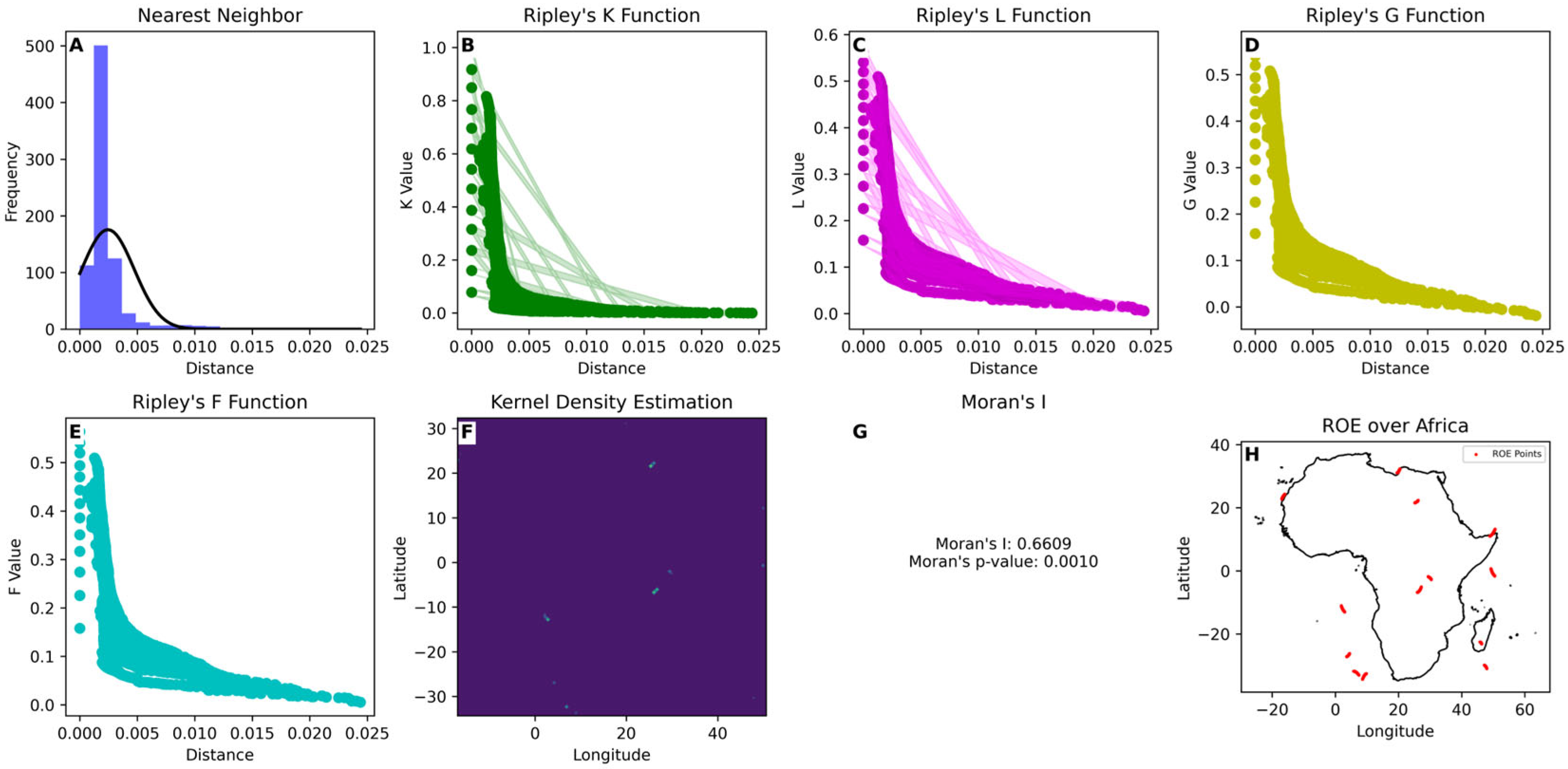
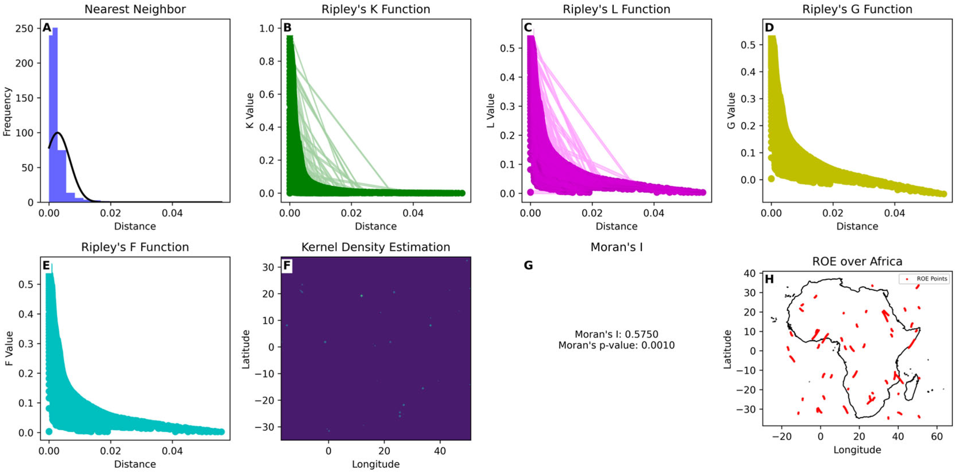
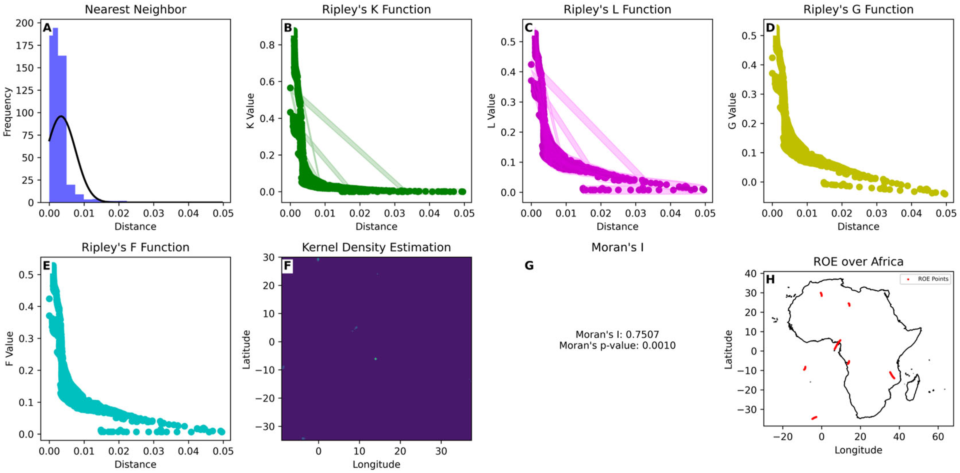
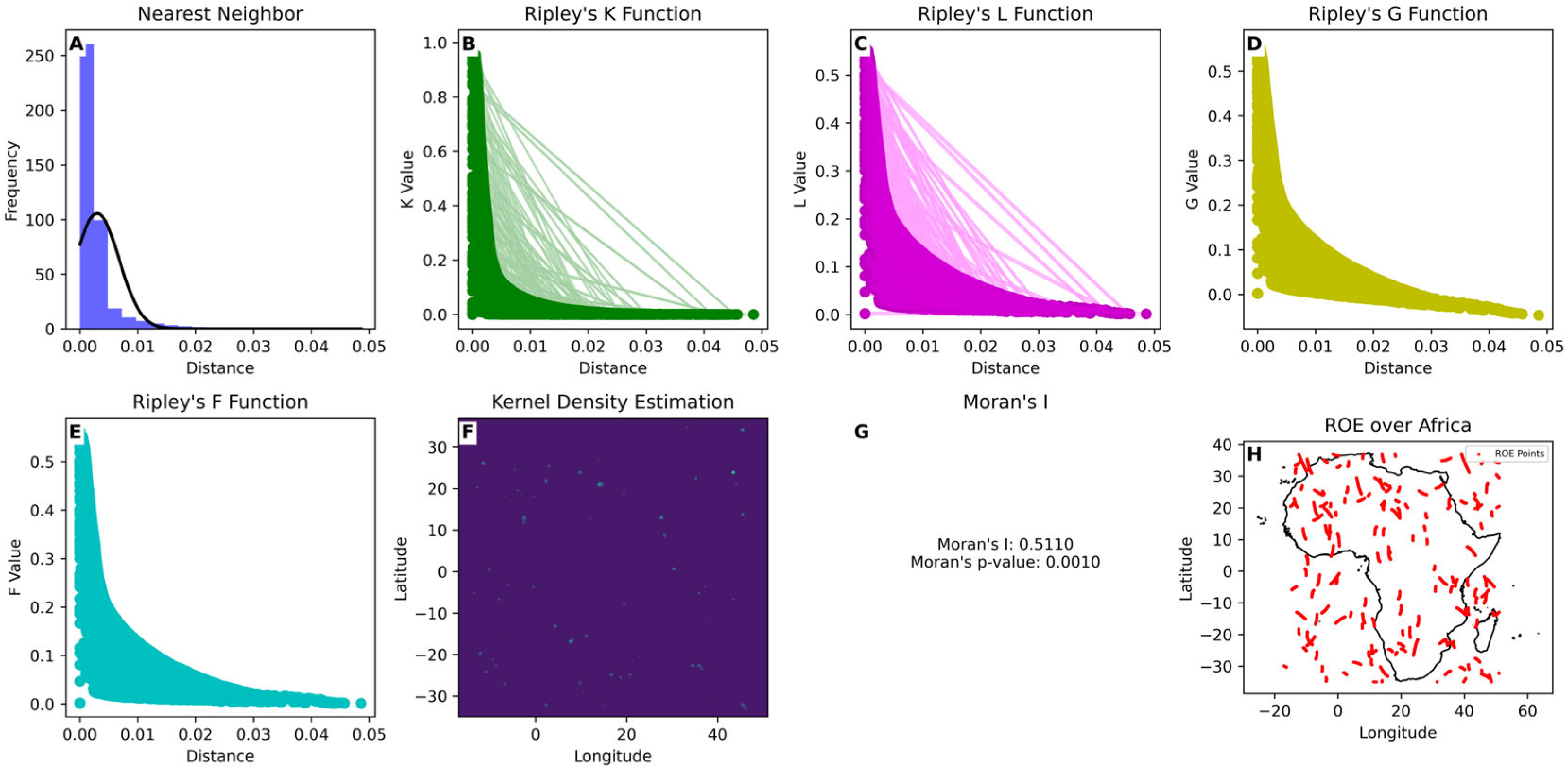
The F-, G-, K-,and L-Functions
3. Results
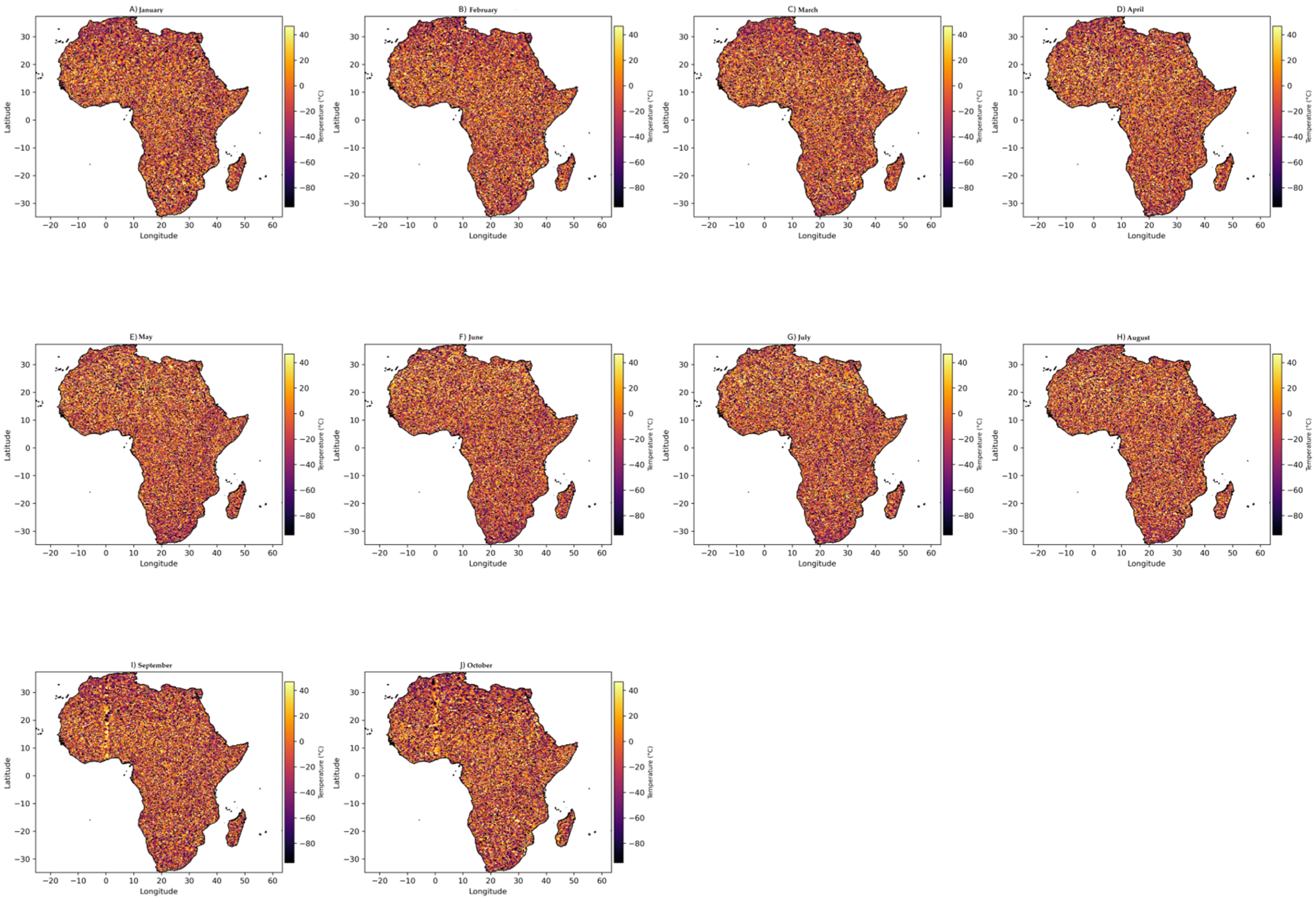
3.1. Spatial Analysis
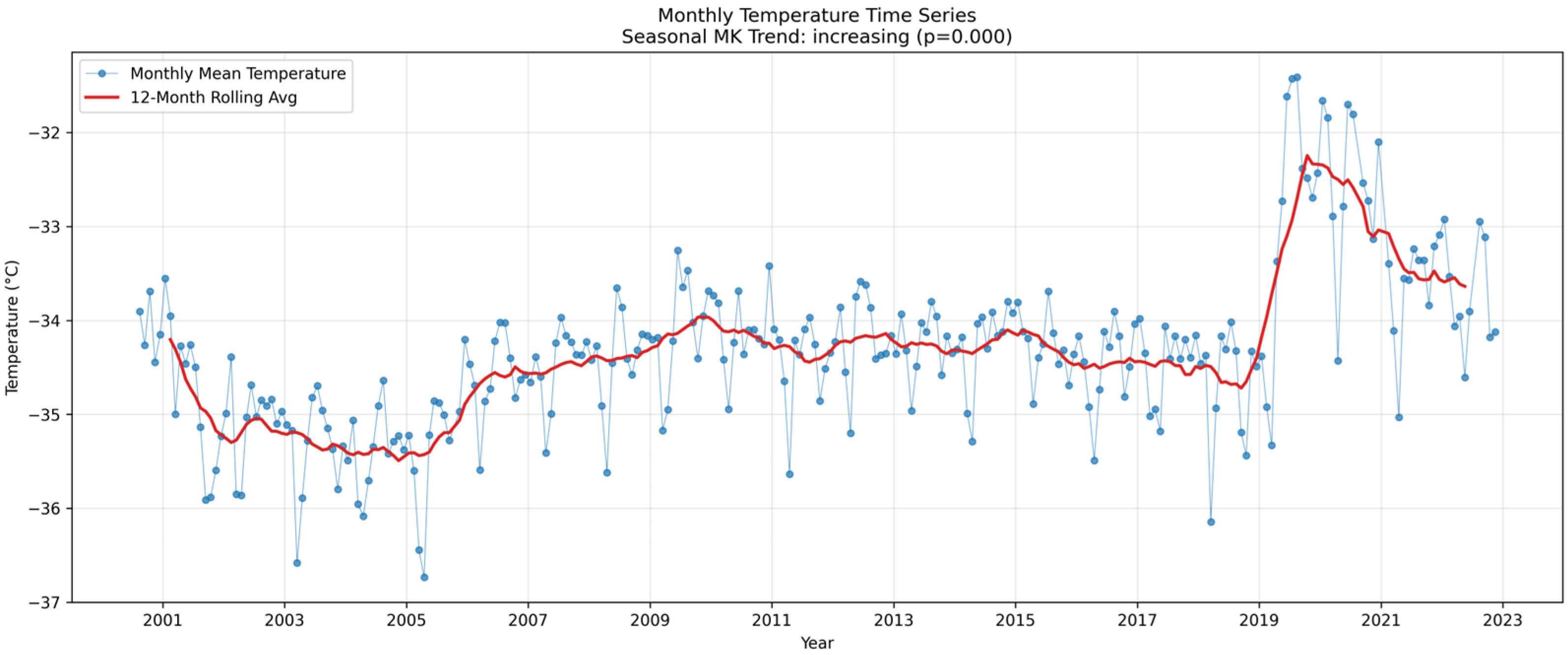
3.2. Temporal Analysis
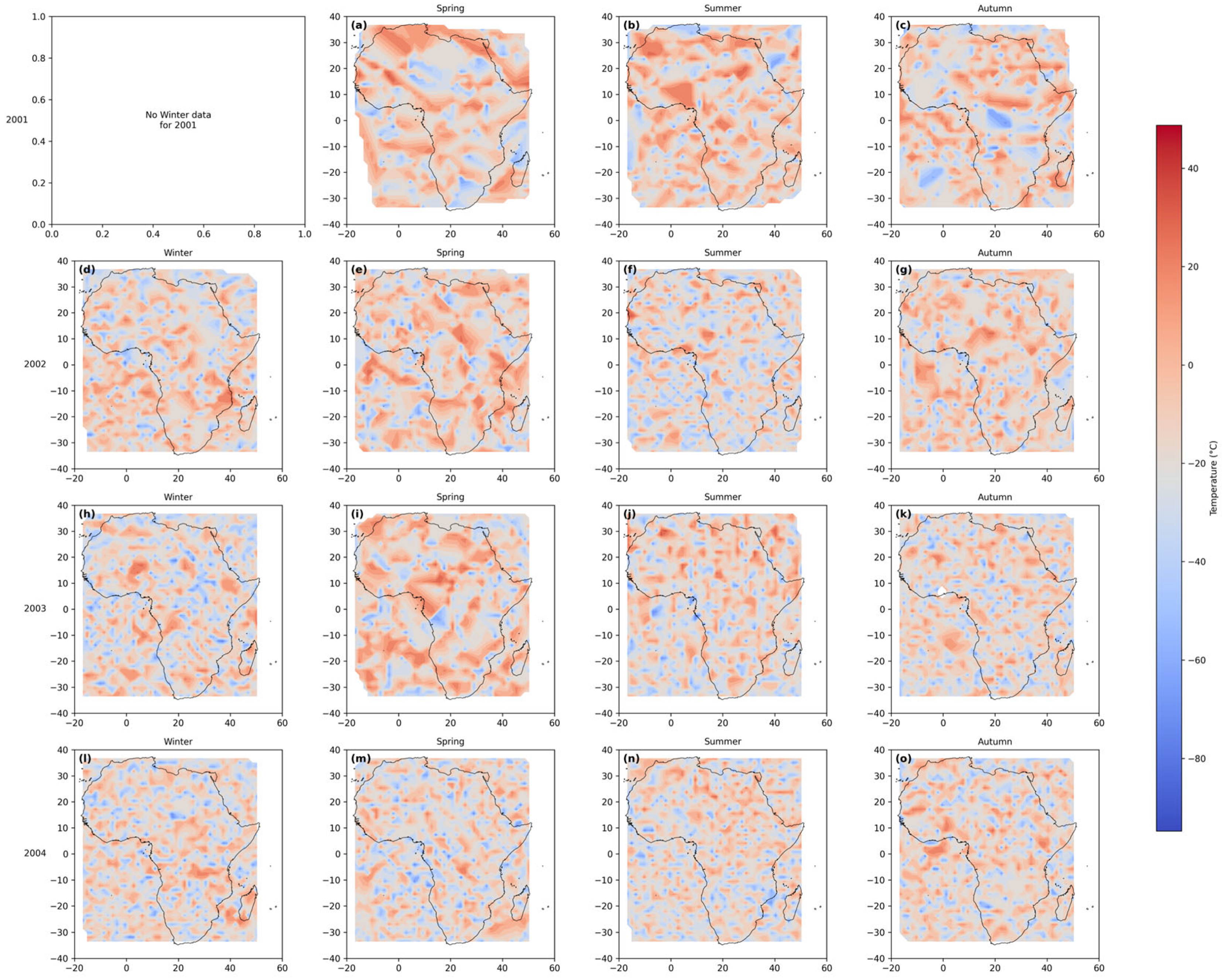
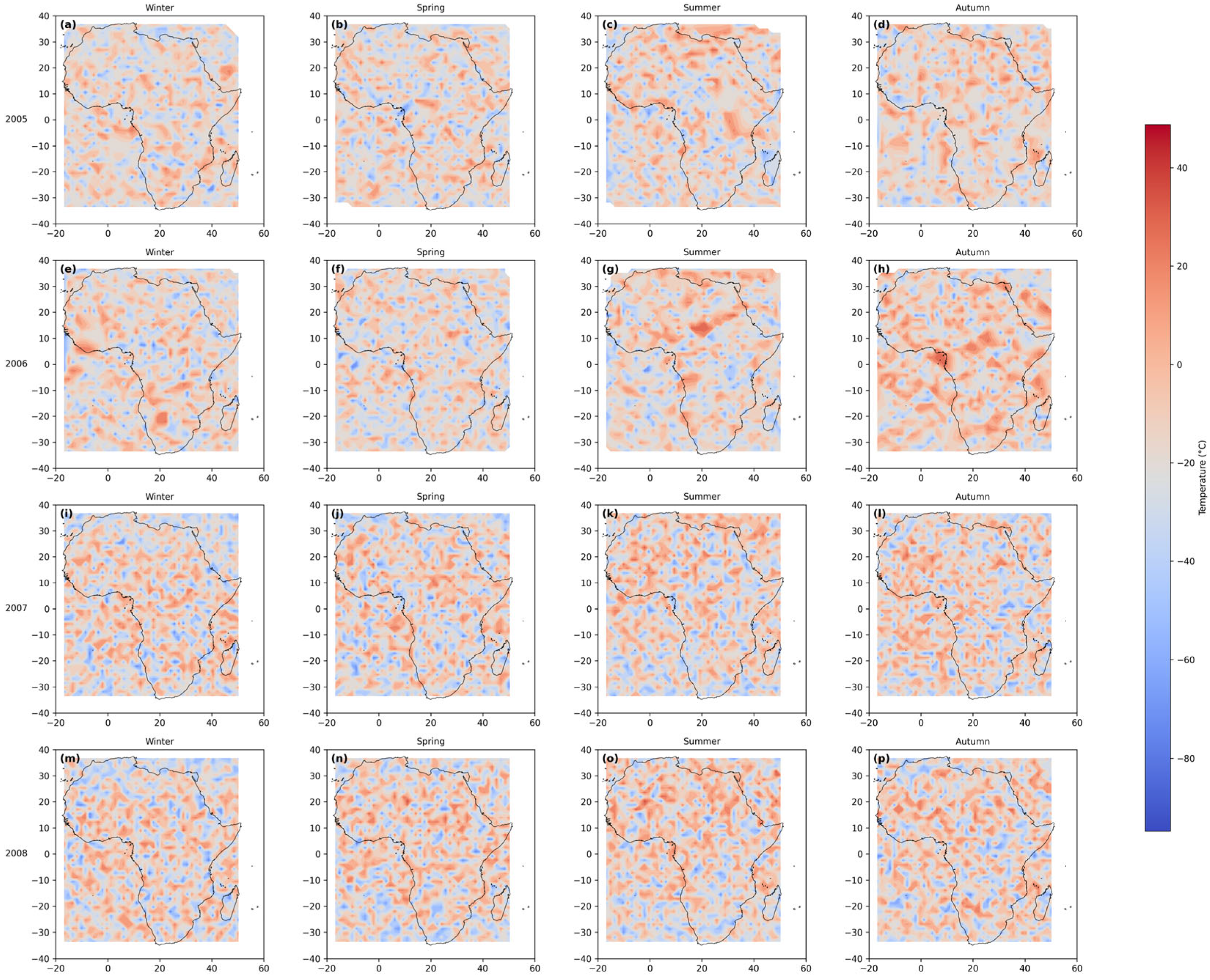
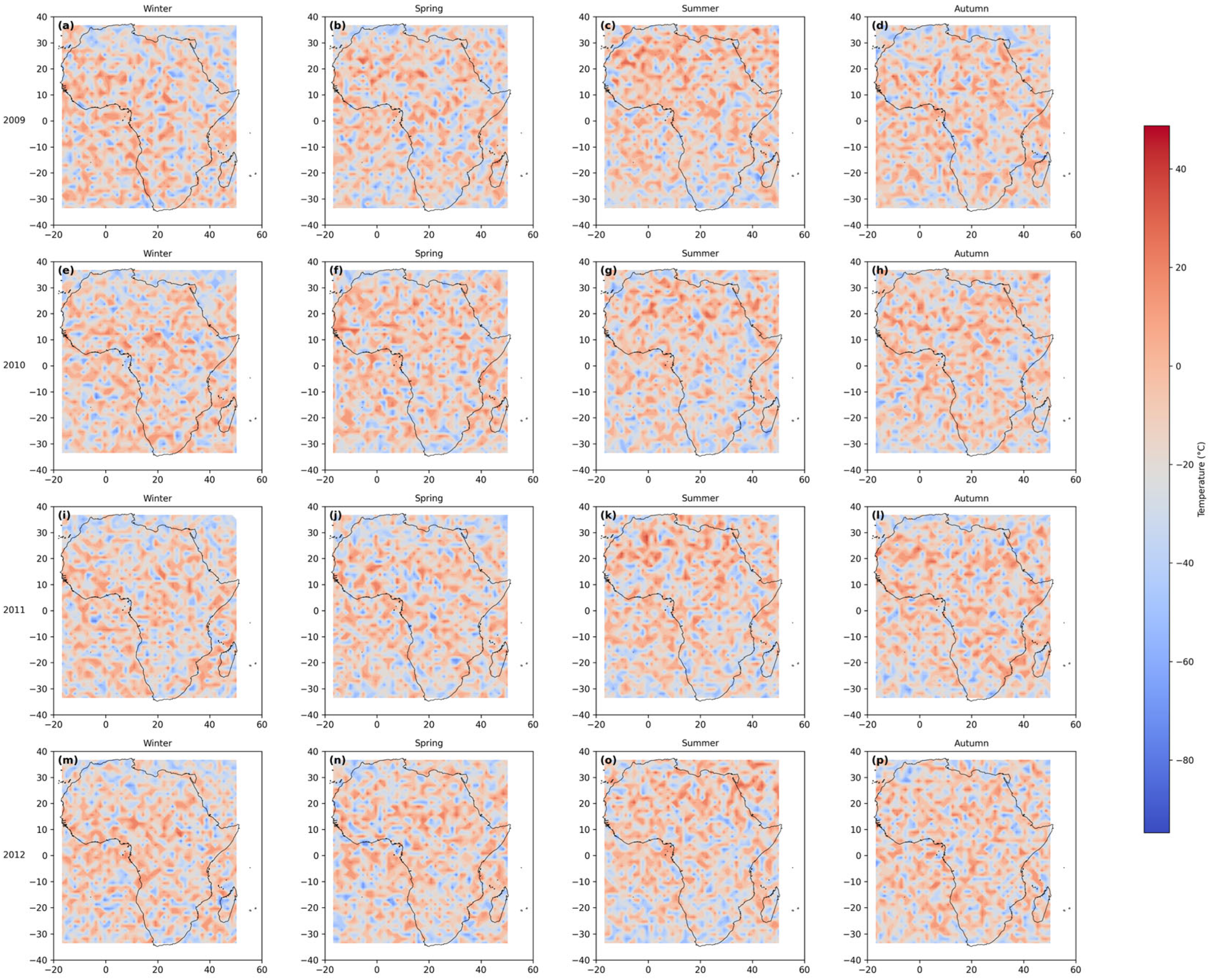
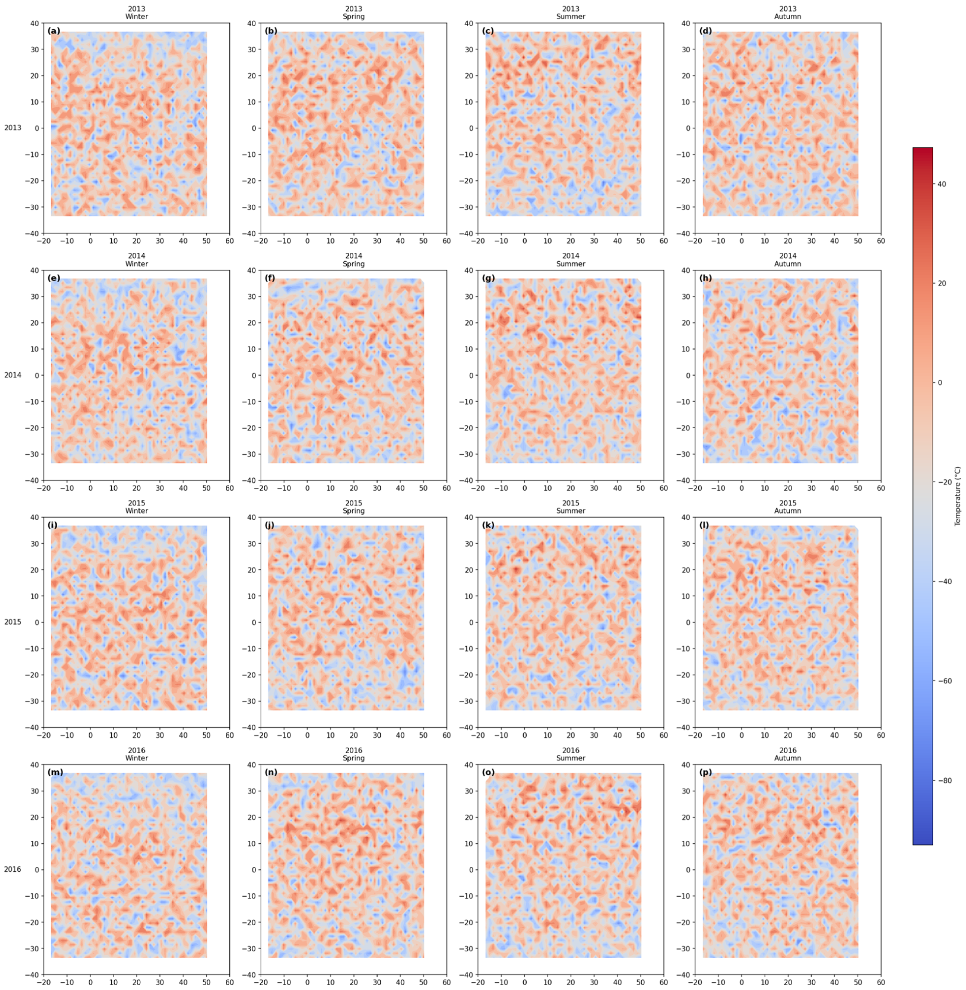
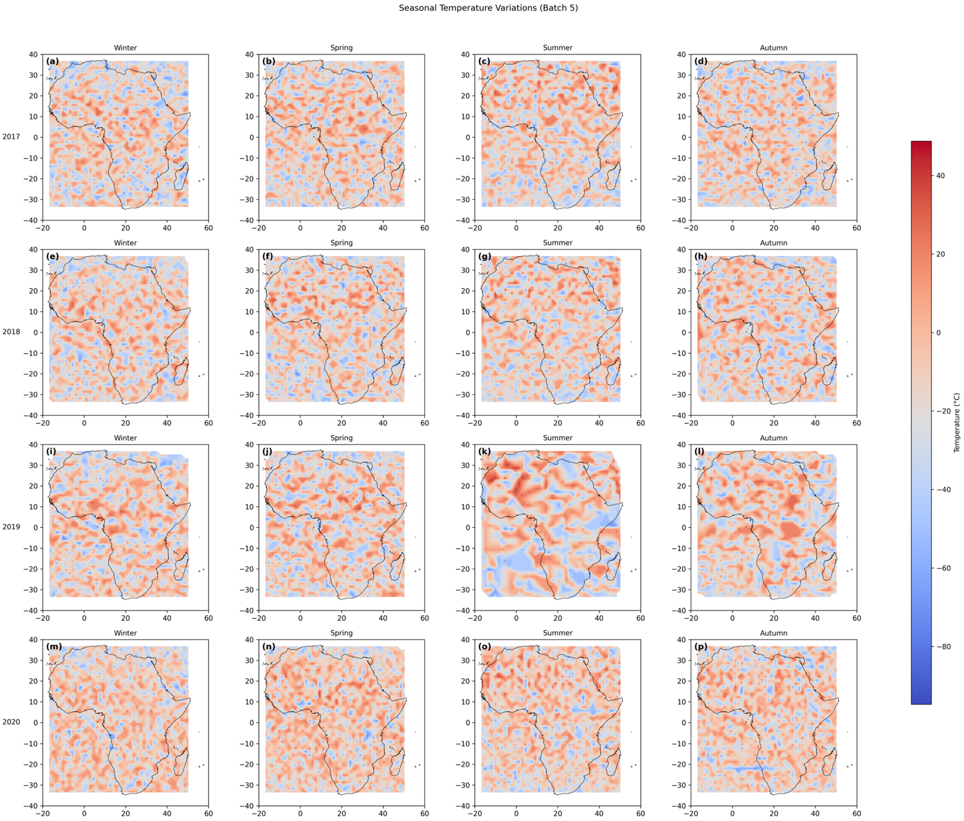
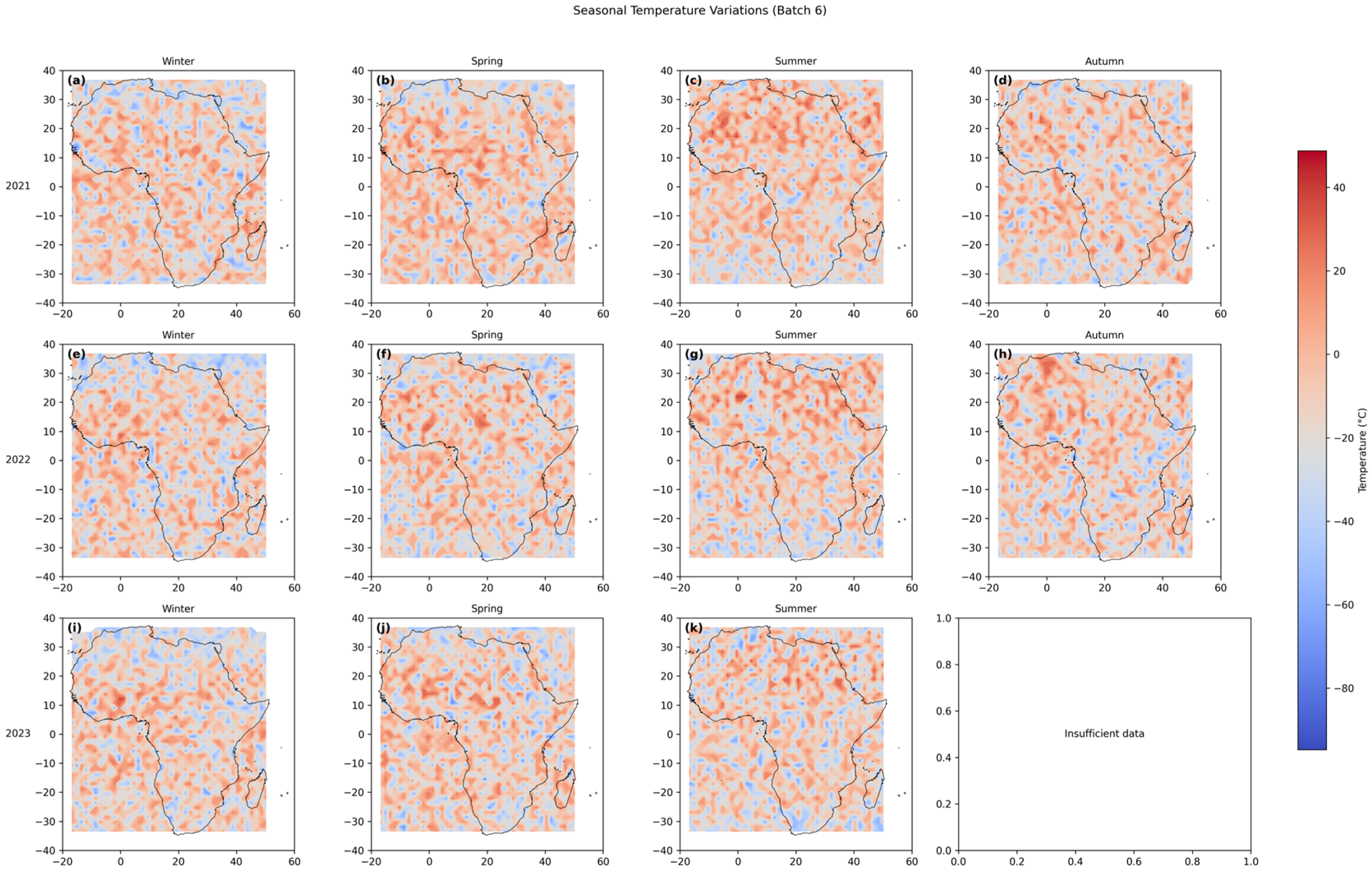
3.3. Seasonal Variation
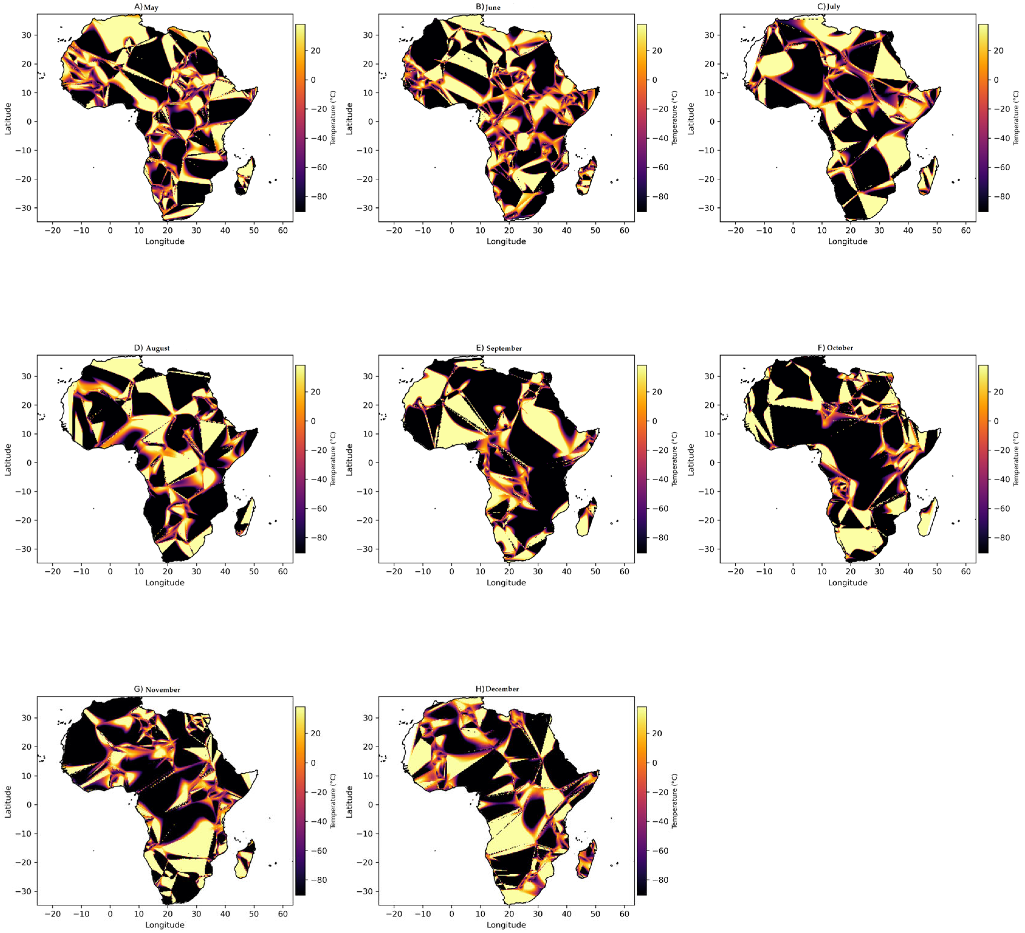
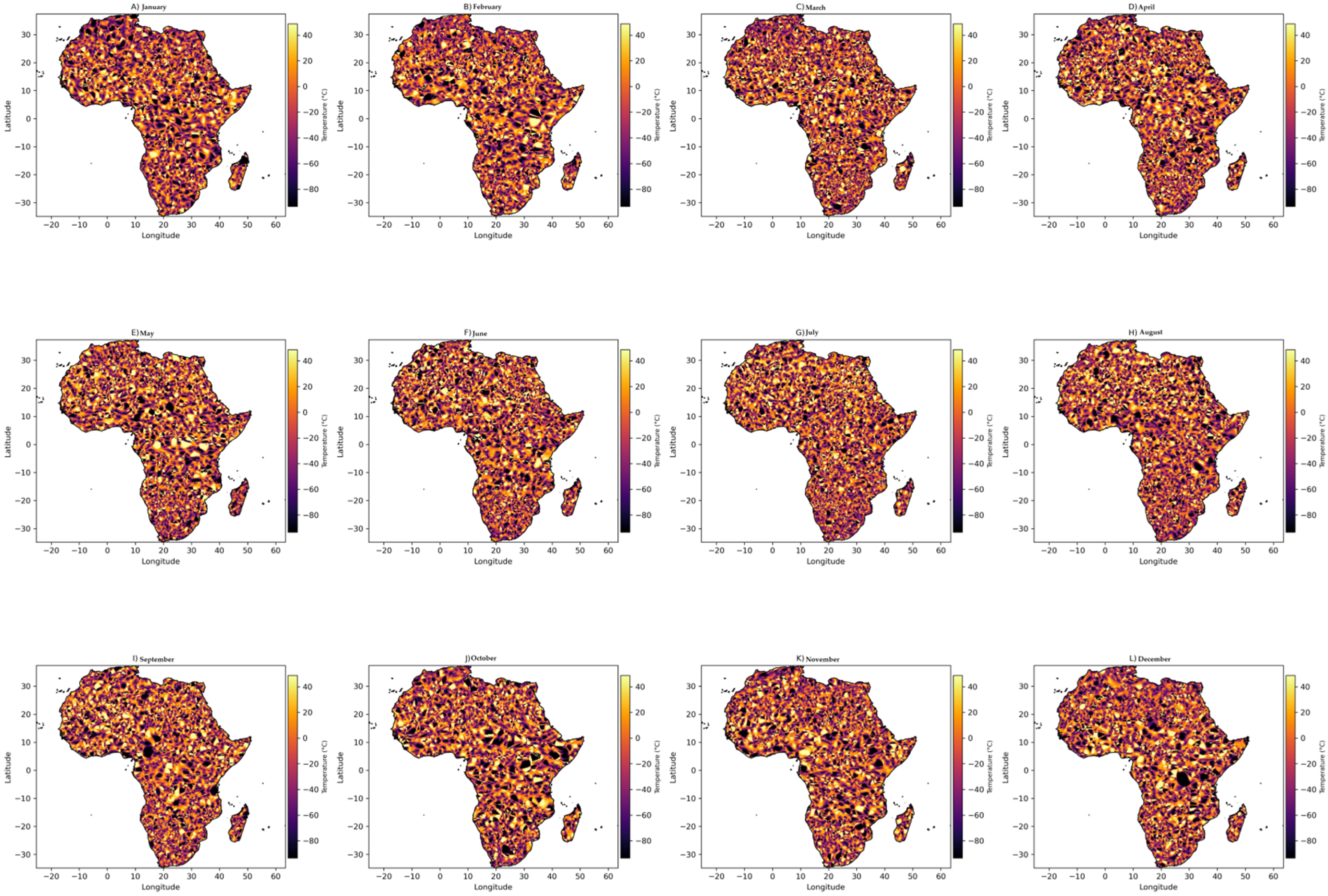
3.4. Heat Map
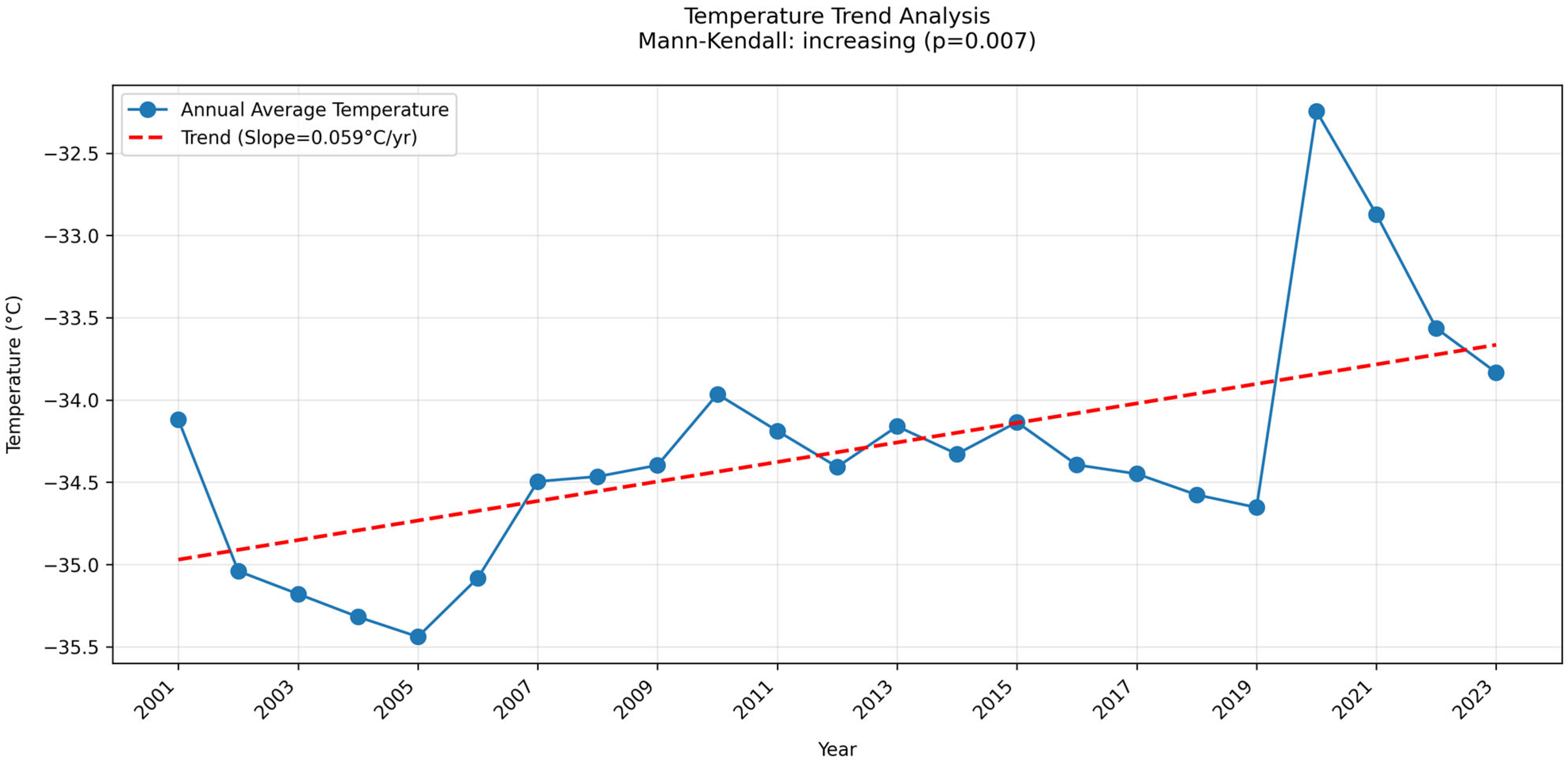
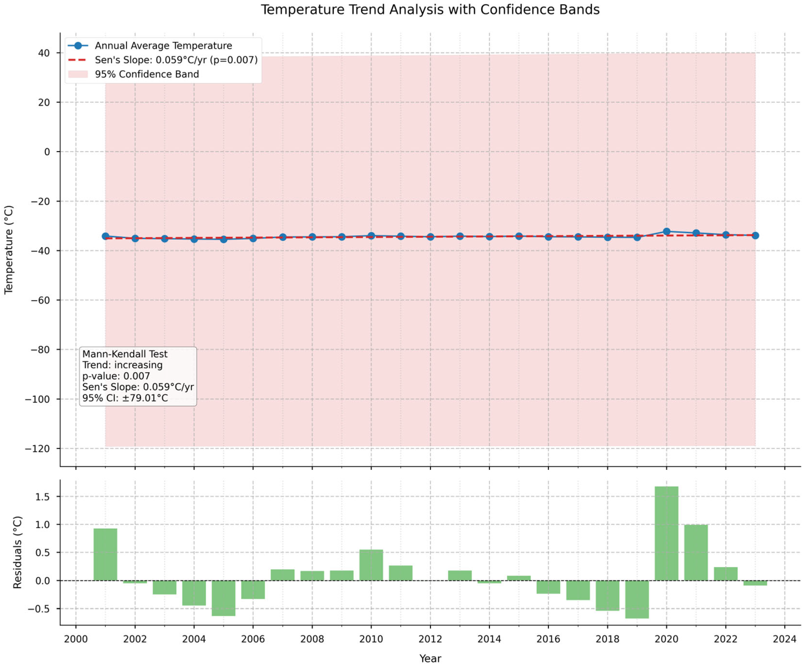
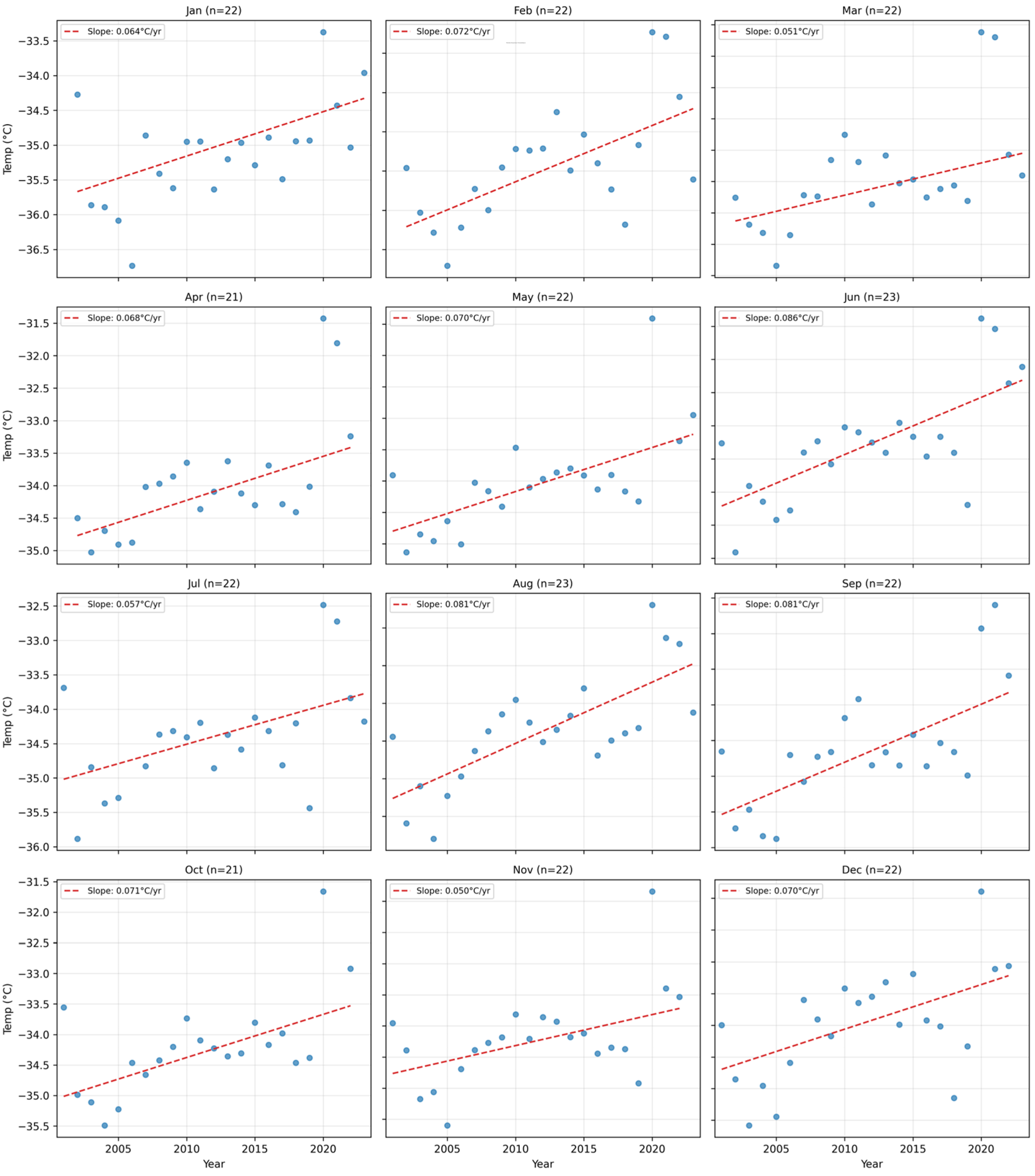
3.5. Trend Analysis
4. Conclusions
5. Recommendations
Author Contributions
Funding
Informed Consent Statement
Data Availability Statement
Conflicts of Interest
References
- Alvar-Beltrán, J. State of the Climate in Africa 2023; UN-iLibrary: New York, NY, USA, 2024. [Google Scholar] [CrossRef]
- Arame, T.; Sarah, L.; Candela, B.V.; Pepukaye, B.; Felipe, M.P.; Elham, S.; Vladimir, S.; Fiona, S.; Samantha, P.; Cindy, P.; et al. Enabling Private Investment in Climate Adaptation & Resilience. 2023. Available online: https://documents1.worldbank.org/curated/en/566041614722486484/pdf/Enabling-Private-Investment-in-Climate-Adaptation-and-Resilience-Current-Status-Barriers-to-Investment-and-Blueprint-for-Action.pdf (accessed on 5 May 2024).
- UNEP. 2023 Adaptation Gap Report. In Press Release: Climate Action; 2023. Available online: https://www.unep.org/resources/adaptation-gap-report-2023 (accessed on 5 May 2024).
- Jamal Saghir, C.; Tapia, M.; Richmond, M. Financial Innovation for Climate Adaptation in Africa DESCRIPTORS Sector Climate Finance Region Global About the Global Center on Adaptation. October 2021. Available online: https://gca.org/wp-content/uploads/2021/10/GCA-CPI-Financial-Innovation-for-Climate-Adaptation-in-Africa.pdf (accessed on 17 December 2023).
- GCACI. State and Trends in Climate Adaptation Finance 2024 About the Global Center on Adaptation. 2024. Available online: https://gca.org/wp-content/uploads/2024/04/State-and-Trends-in-Climate-Adaptation-Finance-2024.pdf (accessed on 22 January 2025).
- Decoding Radio Occultation. The Cornerstone of Accurate Weather Forecasting—Spire: Global Data and Analytics. 2024. Available online: https://spire.com/blog/weather-climate/decoding-radio-occultation-the-cornerstone-of-accurate-weather-forecasting/ (accessed on 14 February 2025).
- WMO. The Global Observing System for Climate: Implementation Needs; World Meteorological Organization: Geneva, Switzerland, 2016.
- WMO. Guide to Climatological Practices, 2018 ed.; Issue WMO-No. 100; World Meteorological Organization: Geneva, Switzerland, 2018. [Google Scholar]
- Yuan, Z.; Noureldeen, N.; Mao, K.; Qin, Z.; Xu, T. Spatiotemporal Change Analysis of Soil Moisture Based on Downscaling Technology in Africa. Water 2022, 14, 74. [Google Scholar] [CrossRef]
- Bi, M.; Wan, L.; Zhang, Z.; Zhang, X.; Yu, C. Spatio-Temporal Variation Characteristics of North Africa’s Climate Potential Productivity. Land 2023, 12, 1710. [Google Scholar] [CrossRef]
- Odhiambo, J.N.; Dolan, C.B.; Troup, L.; Rojas, N.P. Original research: Spatial and spatio-temporal epidemiological approaches to inform COVID-19 surveillance and control: A systematic review of statistical and modelling methods in Africa. BMJ Open 2023, 13, 67134. [Google Scholar] [CrossRef] [PubMed]
- Gleisner, H.; Healy, S.B. Techniques A simplified approach for generating GNSS radio occultation refractivity climatologies. Atmos. Meas. Tech. 2013, 6, 121–129. [Google Scholar] [CrossRef]
- Isioye, O.A.; Combrinck, L.; Botai, J.O.; Munghemezulu, C. The potential for observing African weather with GNSS remote sensing. Adv. Meteorol. 2015, 2015, 723071. [Google Scholar] [CrossRef]
- Scherllin-Pirscher, B.; Steiner, A.K.; Anthes, R.A.; Lexander, M.J.; Alexander, S.P.; Biondi, R.; Birner, T.; Kim, J.; Randel, W.J.; Son, S.-W.; et al. Tropical Temperature Variability in the UTLS: New Insights from GPS Radio Occultation Observations. J. Clim. Am. Meteorol. Soc. 2021, 34, 2813–2839. [Google Scholar] [CrossRef]
- Moses, M.; Ibrahim, U.S.; Akomolafe, E.A. Evaluation of GNSS Radio Occultation Technology for Meteorological and Climate Applications over Nigeria. Evaluation 2023, 7, 461–484. [Google Scholar]
- Taoua, P. Global Africa: Africa in the World and the World in Africa. In African Freedom; Mo Ibrahim Foundation: London, UK, 2018. [Google Scholar]
- Alfred, K.J. Africa|History, People, Countries, Regions, Map, & Facts|Britannica. 2025. Available online: https://www.britannica.com/place/Africa (accessed on 13 January 2025).
- Emeka, A. Africa Dominates List of the World’s 20 Fastest-Growing Economies in 2024—African Development Bank Says in Macroeconomic Report. Www.Afdb.Org. 2024. Available online: https://www.afdb.org/en/news-and-events/press-releases/africa-dominates-list-worlds-20-fastest-growing-economies-2024-african-development-bank-says-macroeconomic-report-68751 (accessed on 16 December 2024).
- Christof, B. Largest Populations in Africa, by Country 2024|Statista. Statista. 2024. Available online: https://www.statista.com/statistics/1121246/population-in-africa-by-country/ (accessed on 17 December 2024).
- Rosenberg, M. The 7 Continents Ranked by Size and Population. 2020. Available online: https://www.thoughtco.com/continents-ranked-by-size-and-population-4163436 (accessed on 17 December 2024).
- Li, L.; Bian, L.; Rogerson, P.; Yan, G. Point Pattern Analysis for Clusters Influenced by Linear Features: An Application for Mosquito Larval Sites. Trans. GIS 2015, 19, 835–847. [Google Scholar] [CrossRef]
- Steinerl, A.K.; Kirchengastl, G.; Foelsche, U.; Kornblueh, L.; Manzinil, E.; Bengtsson, L. GNSS Occultation Sounding for Climate Monitoring. Phys. Chem. Earth Part A Solid Earth Geod. 2001, 26, 113–124. [Google Scholar] [CrossRef]
- Borsche, M.; Gobiet, A.; Steiner, A.K.; Foelsche, U.; Kirchengast, G. Pre-Operational Retrieval of Radio Occultation Based Climatologies. In Atmosphere and Climate: Studies by Occultation Methods; Springer: Berlin/Heidelberg, Germany, 2006; pp. 315–323. [Google Scholar]
- Fu, E. An Investigation of GNSS Radio Occultation Atmospheric Sounding Technique for Australian Meteorology; College of Science, Engineering and Health RMIT University: Melbourne, Australia, 2011. [Google Scholar]
- Thomas, D.S. Adaptation to climate change and variability: Farmer responses to intra-seasonal precipitation trends in South Africa. Clim. Change 2007, 83, 301–322. [Google Scholar] [CrossRef]
- Ngaira, J.K. Impact of Climate Change on Agriculture in Africa by 2030. June 2007. 2014. Available online: https://www.foresightfordevelopment.org/sobipro/54/935-impact-of-climate-change-on-agriculture-in-africa-by-2030 (accessed on 21 April 2023).
- Chad, L. United Nations Fact Sheet on Climate Change Africa is Particularly Vulnerable to the Expected Impacts of Global Warming; Cdm: Bonn, Germany, 2001. [Google Scholar]
- Deressa, T.T. Climate Change and Growth in Africa: Challenges and the Way Forward; The Brookings Institution|Africa Growth Initiative: Washington, DC, USA, 2014; pp. 29–31. [Google Scholar]
- Awojobi, O. The impacts of climate change in Africa: A review of the. J. Int. Acad. Res. Multidiscip. 2017, 5, 39–52. [Google Scholar]
- United Nations Framework Convension on Climate Change. Climate Change Is an Increasing Threat to Africa|UNFCCC. 2020. Available online: https://unfccc.int/news/climate-change-is-an-increasing-threat-to-africa (accessed on 1 February 2023).
- Kottek, M.; Grieser, J.; Beck, C.; Rudolf, B.; Rubel, F. World map of the Köppen-Geiger climate classification updated. Meteorol. Zeitschrif 2006, 15, 259–263. [Google Scholar] [CrossRef] [PubMed]
- Peel, M.C.; Finlayson, B.L.; McMahon, T.A. Updated world map of the Köppen-Geiger climate classification. Hydrol. Earth Syst. Sci. 2007, 11, 1633–1644. [Google Scholar] [CrossRef]
- Beck, H.E.; Zimmermann, N.E.; Mcvicar, T.R.; Vergopolan, N.; Berg, A.; Wood, E.F. Data Descriptor: Present and future Köppen-Geiger climate classification maps at 1-km resolution. Sci. Data 2018, 5, 180214. [Google Scholar] [CrossRef]
- Zadeh, L.A. Fuzzy sets. Inf. Control 1965, 8, 338–353. [Google Scholar] [CrossRef]
- Law, R.; Illian, J.; Burslem, D.F.R.P.; Gratzer, G.; Gunatilleke, C.V.S.; Gunatilleke, I.A.U.N. Ecoogical information from satial patterns of plants: Insights from point process theory. J. Ecol. 2009, 97, 616–628. [Google Scholar] [CrossRef]
- Kempf, M. Modeling multivariate landscape affordances and functional ecosystem connectivity in landscape archeology. Archaeol. Anthropol. Sci. 2020, 12, 159. [Google Scholar] [CrossRef]
- Bilotti, G.; Kempf, M.; Oksanen, E.; Scholtus, L.; Nakoinz, O. Point Pattern Analysis (PPA) as a tool for reproducible archaeological site distribution analyses and location processes in early iron age south-west Germany. PLoS ONE 2024, 19, e0297931. [Google Scholar] [CrossRef]
- Baddeley, A.; Chang, Y.M.; Song, Y.; Turner, R. Nonparametric estimation of the dependence of a spatial point process on spatial covariates. Stat. Its Interface 2012, 5, 221–236. [Google Scholar] [CrossRef]
- Hewitt, R.J.; Wenban-Smith, F.F.; Bates, M.R. Detecting associations between archaeological site distributions and landscape features: A monte carlo simulation approach for the r environment. Geosciences 2020, 10, 326. [Google Scholar] [CrossRef]
- Clark, P.J.; Evans, F.C. Distance to Nearest Neighbor as a Measure of Spatial Relationships in Populations. Ecology 1954, 35, 445–453. [Google Scholar] [CrossRef]
- Kempf, M.; Günther, G. Point pattern and spatial analyses using archaeological and environmental data—A case study from the Neolithic Carpathian Basin. J. Archaeol. Sci. Rep. 2023, 47, 103747. [Google Scholar] [CrossRef]
- Carrero-Pazos, M. Density, intensity and clustering patterns in the spatial distribution of Galician megaliths (NW Iberian Peninsula). Archaeol. Anthropol. Sci. 2019, 11, 2097–2108. [Google Scholar] [CrossRef]
- Diggle, P. A Kernel Method for Smoothing Point Process Data. Appl. Stat. 1985, 34, 138. [Google Scholar] [CrossRef]
- Baxter, M.J.; Beardah, C.C.; Wright, R.V.S. Some archaeological applications of kernel density estimates. J. Archaeol. Sci. 1997, 24, 347–354. [Google Scholar] [CrossRef]
- Sadahiro, Y.; Matsumoto, H. Analysis of a spatial point pattern in relation to a reference point. J. Geogr. Syst. 2024, 26, 351–373. [Google Scholar] [CrossRef]
- Westerholt, R. A Simulation Study to Explore Inference about Global Moran’s I with Random Spatial Indexes. Geogr. Anal. 2023, 55, 621–650. [Google Scholar] [CrossRef]
- Wang, C.C.; Tseng, L.S.; Huang, C.C.; Lo, S.H.; Chen, C.T.; Chuang, P.Y.; Su, N.C.; Tsuboki, K. How much of Typhoon Morakot’s extreme rainfall is attributable to anthropogenic climate change? Int. J. Climatol. 2019, 39, 3454–3464. [Google Scholar] [CrossRef]
- González, J.A.; Moraga, P. Non-Parametric Analysis of Spatial and Spatio-Temporal Point Patterns. R J. 2023, 15, 65–82. [Google Scholar] [CrossRef]
- Cheung, W.H.; Senay, G.B.; Singh, A. Trends and spatial distribution of annual and seasonal rainfall in Ethiopia. Int. J. Climatol. 2008, 28, 1723–1734. [Google Scholar] [CrossRef]
- Smith, S.; Brown, J. Terrestrial Essential Climate Variables: Permafrost and seasonally frozen ground. Global Terrestrial Observing System Version 13 Rome. 2009. Available online: https://scholar.google.com/scholar_url?url=https://citeseerx.ist.psu.edu/document%3Frepid%3Drep1%26type%3Dpdf%26doi%3D1479932112f67c92269e9f1ee3269da7d1e646a0&hl=en&sa=X&ei=AT9IaJajFaalieoP4J3H2A8&scisig=AAZF9b9W7N974pUU2a1VkRsGn9xy&oi=scholarr (accessed on 1 February 2025).
- Ferreira, L.N.; Vega-Oliveros, D.A.; Zhao, L.; Cardoso, M.F.; Macau, E.E.N. Global fire season severity analysis and forecasting. Comput. Geosci. 2020, 134, 104339. [Google Scholar] [CrossRef]
- Spence, C. Explaining seasonal patterns of food consumption. Int. J. Gastron. Food Sci. 2021, 24, 100332. [Google Scholar] [CrossRef]
- El-Shaarawi, A.H.; Piegorsch, W.W. Encyclopedia of Environmetrics; Wiley: Hoboken, NJ, USA, 2002. [Google Scholar]
- Llambi, L.D.; Law, R.; Hodge, A. Temporal changes in local spatial structure of late-successional species: Establishment of an Andean caulescent rosette plant. J. Ecol. 2004, 92, 122–131. [Google Scholar] [CrossRef]
- Vasudevan, K.; Eckel, S.; Fleischer, F.; Schmidt, V.; Cook, F.A. Statistical analysis of spatial point patterns on deep seismic reflection data: A preliminary test. Geophys. J. Int. 2007, 171, 823–840. [Google Scholar] [CrossRef]
- O’Sullivan, D.; Unwin, D.J. Area Objects and Spatial Autocorrelation. In Geographic Information Analysis; John Wiley & Sons: Hoboken, NJ, USA, 2010; pp. 187–214. [Google Scholar] [CrossRef]
- O’Sullivan, D.; Unwin, D.J. Geographic Information Analysis and Spatial Data. In Geographic Information Analysis; John Wiley & Sons: Hoboken, NJ, USA, 2010; pp. 1–32. [Google Scholar] [CrossRef]
- O’Sullivan, D.; Unwin, D.J. Practical Point Pattern Analysis. In Geographic Information Analysis; John Wiley & Sons: Hoboken, NJ, USA, 2010; pp. 157–186. [Google Scholar] [CrossRef]
- O’Sullivan, D.; Unwin, D.J. The Pitfalls and Potential of Spatial Data. In Geographic Information Analysis; John Wiley & Sons: Hoboken, NJ, USA, 2010; pp. 33–54. [Google Scholar] [CrossRef]
- Dixon, P.M.; El-shaarawi, A.H.; Piegorsch, W.W. Nearest Neighbor Methods. Encycl. Mach. Learn. 2011, 3, 715. [Google Scholar] [CrossRef]
- Diggle, P.J. Statistical Analysis of Spatial and Spatio-Temporal Point Patterns; CRC Press: Boca Raton, FL, USA, 2023. [Google Scholar]
- Diggle, P.J.; Moraga, P.; Rowlingson, B.; Taylor, B.M. Spatial and spatio-temporal log-gaussian cox processes: Extending the geostatistical paradigm. Stat. Sci. 2013, 28, 542–563. [Google Scholar] [CrossRef]
- Smith, W.W. Nearest neighbor analysis, tourism. In Encyclopedia of Tourism; Springer: Cham, Switzerland, 2015; pp. 1–2. [Google Scholar] [CrossRef]
- Sadahiro, Y. Comparison and Classification of Multiple Distributions of Points. J. City Plan. Inst. Jpn. 2016, 51, 929–936. [Google Scholar] [CrossRef]
- Sadahiro, Y. Statistical analysis of spatial segregation of points. Comput. Environ. Urban Syst. 2019, 76, 123–138. [Google Scholar] [CrossRef]
- Sadahiro, Y. A method for analyzing the daily variation in the spatial pattern of market area. J. Retail. Consum. Serv. 2021, 58. [Google Scholar] [CrossRef]
- Sadahiro, Y.; Liu, Y. A scale-sensitive approach for comparing and classifying point patterns. J. Spat. Sci. 2020, 65, 281–306. [Google Scholar] [CrossRef]
- Müller, R.; Kunz, A.; Hurst, D.F.; Rolf, C.; Krämer, M.; Riese, M. The need for accurate long-term measurements of water vapor in the upper troposphere and lower stratosphere with global coverage. Earth’s Future 2016, 4, 25–32. [Google Scholar] [CrossRef] [PubMed]
- González, J.A.; Rodríguez-Cortés, F.J.; Cronie, O.; Mateu, J. Spatio-temporal point process statistics: A review. Spat. Stat. 2016, 18, 505–544. [Google Scholar] [CrossRef]
- De Paor, D.G.; Dordevic, M.M.; Karabinos, P.; Burgin, S.; Coba, F.; Whitmeyer, S.J. Exploring the reasons for the seasons using Google Earth, 3D models, and plots. Int. J. Digit. Earth 2017, 10, 582–603. [Google Scholar] [CrossRef]
- Bilbao, J.; Román, R.; De Miguel, A. Temporal and spatial variability in surface air temperature and diurnal temperature range in Spain over the period 1950–2011. Climate 2019, 7, 16. [Google Scholar] [CrossRef]
- Boots, B.N.; Getis, A. Point Pattern Analysis; Thrall, G.I., Ed.; WVU Research Repository. 2020. Available online: https://researchrepository.wvu.edu/rri-web-book/13/ (accessed on 1 February 2025).
- Elrahman Yassien, A.; El-Kutb Mousa, A.; Rabah, M.; Saber, A.; Zhran, M. Analysis of spatial and temporal variation of precipitable water vapor using COSMIC radio occultation observations over Egypt. Egypt. J. Remote Sens. Space Sci. 2022, 25, 751–764. [Google Scholar] [CrossRef]


| S/N | Missions | Date | Status | Country | Altitude (Km) | Inclination Angle (°) | Coverage |
|---|---|---|---|---|---|---|---|
| 1 | CHAMP | 2001–2008 | Non-operational | Germany | 454 | 87.3 | Global |
| 2 | GRACE | 2007–2017 | Non-operational | Germany | 485 | 89 | Global |
| 3 | COSMIC-1 | 2006–2019 | Non-operational | Taiwan | 800 | 72 | Global |
| 4 | TERRASAR-X | 2008–2019 | Operational | Germany | 514.8 | 79.5 | Global |
| 5 | CNOFS | 2010–2015 | Non-operational | USA | 464 | 13 | Global |
| 6 | KOMPSAT5 | 2015–2019 | Operational | Korea | 550 | 97.6 | Global |
| 7 | PAZ | 2018–2019 | Operational | Spain | 514 | 97.4 | Global |
| 8 | SACC | 2006–2011 | Non-operational | Argentina | 702 | 98 | Global |
| 9 | METOP-A | 2007–2015 | Non-operational | Europe | 827 | 98.7 | Global |
| 10 | METOP-B | 2013–2019 | Operational | Europe | 827 | 98.7 | Global |
| 11 | METOP-C | 2019–now | Operational | Europe | 817 | 98.7 | Global |
| 12 | COSMIC-2 | 2019–now | Operational | Taiwan | 800 | 72 | Global |
Disclaimer/Publisher’s Note: The statements, opinions and data contained in all publications are solely those of the individual author(s) and contributor(s) and not of MDPI and/or the editor(s). MDPI and/or the editor(s) disclaim responsibility for any injury to people or property resulting from any ideas, methods, instructions or products referred to in the content. |
© 2025 by the authors. Licensee MDPI, Basel, Switzerland. This article is an open access article distributed under the terms and conditions of the Creative Commons Attribution (CC BY) license (https://creativecommons.org/licenses/by/4.0/).
Share and Cite
Ibrahim, U.S.; Aleem, K.; Musa, T.A.; Youngu, T.T.; Obadaki, Y.Y.; Wan Aris, W.A.; Kang Wee, K.T. An Investigation of GNSS Radio Occultation Data Pattern for Temperature Monitoring and Analysis over Africa. NDT 2025, 3, 15. https://doi.org/10.3390/ndt3020015
Ibrahim US, Aleem K, Musa TA, Youngu TT, Obadaki YY, Wan Aris WA, Kang Wee KT. An Investigation of GNSS Radio Occultation Data Pattern for Temperature Monitoring and Analysis over Africa. NDT. 2025; 3(2):15. https://doi.org/10.3390/ndt3020015
Chicago/Turabian StyleIbrahim, Usman Sa’i, Kamorudeen Aleem, Tajul Ariffin Musa, Terwase Tosin Youngu, Yusuf Yakubu Obadaki, Wan Anom Wan Aris, and Kelvin Tang Kang Wee. 2025. "An Investigation of GNSS Radio Occultation Data Pattern for Temperature Monitoring and Analysis over Africa" NDT 3, no. 2: 15. https://doi.org/10.3390/ndt3020015
APA StyleIbrahim, U. S., Aleem, K., Musa, T. A., Youngu, T. T., Obadaki, Y. Y., Wan Aris, W. A., & Kang Wee, K. T. (2025). An Investigation of GNSS Radio Occultation Data Pattern for Temperature Monitoring and Analysis over Africa. NDT, 3(2), 15. https://doi.org/10.3390/ndt3020015