In Pursuit of Samuelson for Commodity Futures: How to Parameterize and Calibrate the Term Structure of Volatilities

Abstract

The phenomenon of rising forward price volatility, both historical and implied, as maturity approaches is referred to as the Samuelson effect or maturity effect. Disregarding this effect leads to significant mispricing of early-exercise options, extendible options, or other path-dependent options. The primary objective of the research is to identify a practical way to incorporate the Samuelson effect into the evaluation of commodity derivatives. We choose to model the instantaneous variance employing the exponential decay parameterizations of the Samuelson effect. We develop efficient calibration techniques utilizing historical futures data and conduct an analysis of statistical errors to provide a benchmark for model performance. The study employs 15 years of data for WTI, Brent, and NG, producing excellent results, with the fitting error consistently inside the statistical error, except for the 2020 crisis period. We assess the stability of the fitted parameters via cross-validation techniques and examine the model’s out-of-sample efficacy. The approach is generalized to encompass seasonal commodities, such as natural gas and electricity. We illustrate the application of the calibrated model of instantaneous variance for the evaluation of commodity derivatives, including swaptions, as well as in the evaluation of power purchase agreements (PPAs). We demonstrate a compelling application of the Samuelson effect to a widely utilized auto-callable equity derivative known as the snowball.

1. Introduction

Understanding the dynamics of futures price volatility is very important for many aspects of risk management, such as hedging, portfolio construction, derivative pricing, etc. Samuelson was the first to investigate the relationship between volatility and time until contract expiration, stating the hypothesis that the volatility of futures price changes should increase as the delivery date nears. This prediction is very well-known and referred to as the Samuelson hypothesis or maturity effect [1]. This backwardation of volatility of forward contracts arises across most markets, but this effect is especially pronounced in energy markets as a particular steep increase in volatility occurs in the last six (or less) months of the life of the contract. This is one of the most fascinating phenomena of commodity futures, which must be taken into account in pricing and managing of commodity contracts.

The primary objective of our article is to provide a method to parameterize and, more crucially, calibrate the rise in volatility as contract maturity approaches. We are not questioning the validity of the Samuelson effect for the examined commodity futures, nor do we model the entire volatility surface, which involves stochastic volatility models. We focus only on the Samuelson effect and seek a viable solution that yields stable results. Our primary objective is to identify a natural and practical way to integrate the Samuelson effect in the evaluation of path-dependent options, early-expiry options, CVA, and related matters. Consequently, we chose instantaneous variance of commodity futures as the focus of the study. This choice allows us to match the market information, such as option quotes on futures, perfectly (via implied volatilities).

We begin with a simple example that demonstrates the importance of the Samuelson effect and the consequences of ignoring it. We consider a future contract on WTI with expiration in $T=2$ years priced at $F(0,T)=$ USD 64 per barrel. Assume that the implied volatility quoted for this contract is ${\sigma }_{imp}=35\%$, and we consider an ATM call option on this future expiring $\tau =3$ months before the contract expiration, thus in $T-\tau =1.75$ years. Such options are called early-exercise options. The total variance during the lifetime of the contract will be $va{r}_{total}={\sigma }_{imp}^{2}T=0.245$. If we price the option using the quoted implied volatility, the price of the early-exercise ATM call option will be USD $11.72$ per unit (no discount). However, under the Samuelson effect, the variance does not accumulate in a uniform fashion, so such a calculation will be wrong. Suppose we have a strong Samuelson such that half of the total variance happens in the last three months of the life of the contract. In such a case, to price the option, we have to use the following volatility:

$${\sigma }_1=\sqrt{{\displaystyle \frac{0.5va{r}_{total}}{T-\tau }}}=26.46\%$$

The right option price is USD $8.89$, and ignoring the presence of Samuelson leads to overpricing the option by $32\%$.

Now, let us analyze the consequences of using a wrong variance for the second part of the time, the last three months of the lifetime of the contract. Since half of the total variance realizes during a short period of time of three months, the average volatility ${\sigma }_2$ corresponding to the last three months will be much higher:

$${\sigma }_2=\sqrt{{\displaystyle \frac{0.5va{r}_{total}}{\tau }}}=70\%$$

Assume that in $1.75$ years we have a right to buy a call option for premium $X_2=$ USD 10, and the strike $X_1$ of the call option is equal to the current forward price $X_1=F(0,T)$. Thus, we consider a compound option with payoff

$$c_{comp}=max\left(c_{BL}(F(T-\tau ,T),X_1,{\sigma }_2,\tau )-X_2,0\right)$$

where $c_{BL}(F,X,{\sigma }_2,\tau )$ is the Black call price with price F of the underlying asset, strike $X_1$, volatility ${\sigma }_2$, and time to expiration $\tau$. We can price the compound option by using standard numerical procedures (grid evaluation or Monte Carlo). Even though the right ${\sigma }_2$ with Samuelson is higher than with flat Samuelson, the expectation of the underlying call option $c_{BL}$ is the same in the two scenarios (we use risk-neutral pricing). However, the distribution of futures prices in $1.75$ years with flat Samuelson is much wider (standard deviation of futures price of USD $31.37$ vs. USD $23.06$), which makes the compound option more expensive under flat Samuelson $c_{comp}=$ USD $8.32$ vs. with Samuelson $c_{comp}=$ USD $6.41$. Disregarding Samuelson results in overpricing the option by $30\%$.

Another example of an early-exercise option includes swaptions, which are widespread products in energy markets. Their evaluation is discussed in [2]; see also the recent book on quantitative trading in the oil market by Bouchoev [3]. The Samuelson effect must be taken into account in the evaluation of path-dependent options, such as extendibles, calculations of forward exposure of a portfolio (necessary for CVA computations), hedging decisions, etc.

We now provide a comprehensive summary of the current research on the subject, which includes the most recent developments.

Empirical analyses have been conducted on the Samuelson hypothesis in numerous studies, and it has been validated in a subset of markets. Many of them reach mixed conclusions. For example, Miller [4] investigates live cattle, Barnhill et al. [5] study U.S. Treasury bonds; Adrangi et al. [6] consider selected energy; Adrangi and Chatrath [7] analyze coffee, sugar, and cocoa. Andersen [8] finds evidence in the agricultural markets, such as wheat, oats, soybean meal, and cocoa, but not for silver. Milonas [9] finds strong support for the hypothesis in agricultural markets, but little or no support when using gold, copper, GNMA, T-bond, and T-bill prices. Rutledge [10] finds support for the Samuelson hypothesis with silver and cocoa, but inconclusive evidence for wheat and soybean oil. Galloway and Kolb [11] study the term structure of volatility in 45 markets, including agricultural and energy commodity futures, precious and industrial metal futures, and stock index, currency, and interest rate futures. Their findings provide support for the maturity effect in agricultural and energy commodities, but not in precious metals and financials. Liu [12] employs almost stochastic dominance and the power spectrum to investigate the maturity effect for five groups of energy futures, such as crude oil, reformulated regular gasoline, RBOB regular gasoline, No. 2 heating oil, and propane. The outcome provides mixed results, ranging from supporting to being contrary to the hypothesis. Jaeck and Lautier [13] find evidence of a Samuelson effect in various electricity markets, such as German, Nordic, Australian, and US, and show that storage is not a necessary condition for such an effect to appear. A recently published article by Castello [14] examines the term structure dynamics in the natural gas futures market, specifically analyzing the daily futures price of the Dutch Title Transfer Facility (TTF) via a machine-learning-based methodology, providing evidence supporting the Samuelson hypothesis.

“Negative” papers rejecting the hypothesis include Grammatikos and Saunders [15], who find no relationship between futures return volatility and time-to-maturity for currency futures prices, and a study by Park and Sears [16] provides evidence to disprove the Samuelson hypothesis for stock indices. The well-known study by Bessembinder et al. [17] suggests that the hypothesis will be generally supported in markets where spot price changes include a predictable temporary component, which is more likely to be met in real assets than for financial assets. They show that the hypothesis will generally be supported in markets where spot prices and convenience yields are positively correlated. The authors assume that the carry arbitrage model represents futures markets.

The carry arbitrage model is based on the notion that the underlying instrument can be “carried” (purchased) with $100\%$ financing (borrowing) and delivered against a short futures position. Brooks [18] identifies and explores the important link between the empirical Samuelson hypothesis and theoretical carry: the degree to which carry arbitrage is empirically validated is associated with the degree to which the Samuelson hypothesis is not supported. In the continuation of the research, Brooks and Teterin [19] study the volatility-term structure in 10 futures markets comprising three categories: agriculture, energy, and metals. To estimate the slope of the volatility-term structure, they use the Nelson and Siegel [20] functional form, borrowed from the literature on modeling the term structure of interest rates. The authors show that the slope of the volatility-term structure is more negative when inventories are low, and that the threshold for high/low inventory is specific to each market. The relationship between the Samuelson hypothesis and inventory levels is rooted in the cost-of-carry model.

The popular models in the academic literature arrive at the Samuelson effect of futures volatility by considering models formulated in terms of the spot energy price with mean reverting process; see Clewlow and Strickland [21]. The Schwatz single-factor model [22] results in the exponential decay of future volatility:

$${\sigma }_F(t,T)=\sigma e^{-\alpha (T-t)}$$

(1)

where $\alpha$ is the mean reversion rate, and $\sigma$ is the spot-price volatility. The long-term level of volatilities at $T=\infty$ is zero, which is not realistic. Two-factor models with mean reverting processes for spot price and convenience yield (see Schwartz [22]. Gibson and Schwartz [23], and Pilipović [24]) result in an exponential decay of futures volatility with non-zero long-term level volatility at long horizons.

The vital paper by Schwartz and Trolle [25] expands the framework of spot models to accommodate unspanned stochastic volatility. In their approach, the volatility of both spot price and forward cost of carry depend on two volatility factors that follow a mean reverting process, resulting in the Samuelson effect for futures volatility. Crosby and Frau [26] broaden the model in [25] by incorporating multiple jump processes. They explore the valuation of plain vanilla options on futures prices when the spot price follows a log-normal process, the forward cost of carry curve and the volatility are stochastic variables, and the spot price and forward cost of carry allow for time-dampening jumps. Frau and Fanelli [27] present a new term-structure model for commodity futures prices based on [25], which they extend by incorporating seasonal stochastic volatility represented with two different sinusoidal expressions and price plain vanilla options on the Henry Hub natural gas futures contracts. Hillard and Hillard [28] develop a jump-diffusion model for pricing and hedging with margined options on futures. They introduce a jump-diffusion process for spot prices, and mean reverting processes for interest rate and stochastic convenience yield. Under positive correlations between diffusion parts, futures volatility increases as maturity approaches. Model parameters are calibrated using data on Brent crude contracts.

Another class of models addresses the direct modeling of futures rather than relying on spot pricing and unobservable convenience yield. Chiarella et al. [29] propose a model encompassing hump-shaped unspanned stochastic volatility, which entails a finite-dimensional affine model for the commodity futures curve and quasi-analytical prices for options on commodity futures. Schnieder and Tavin [30] introduce a futures-based model capable of capturing the main features displayed by crude oil futures and options contracts, such as the Samuelson volatility effect and the volatility smile. They calculate the joint characteristic function of two futures contracts in the model in analytic form and use it to price calendar spread options.

In the contemporary analysis of commodity volatility, it is imperative to take into account both geopolitical and climate risks. For instance, a recent study by Özdemir et al. [31] examines the influence of the Geopolitical Risk Index (GPR) on the volatility of commodity futures returns. It broadens the scope of the research to encompass industrial metals, energy, agricultural products, and precious metals. Another recent paper by Guo et al. [32] introduces a climate change concern index to quantify climate risk and evaluate its impact on commodity futures volatility.

We will now delineate the fundamental concepts of our methodology and compare them with existing techniques.

We opt to utilize futures data and model their instantaneous variance using exponential decay models as the majority of commodity trading happens in futures markets. A natural generalization of (1), explicitly shown in many publications (see, for instance, [30] or [3]), is the following form of variance parameterization including two exponential decays:

$${\sigma }_F^2(t,T)={\sigma }_0^2\left(e^{-2B(T-t)}+{\sigma }_{\infty }^2{e}^{-2\beta (T-t)}\right)$$

(2)

where B is the global decay and $\beta$ is a long-term decay (much smaller than B); ${\sigma }_0$ is the normalization factor to match the implied market volatility, and ${\sigma }_{\infty }$ is the level of a long-term volatility. Swindle [33] uses this representation to model the total implied variance of commodity futures.

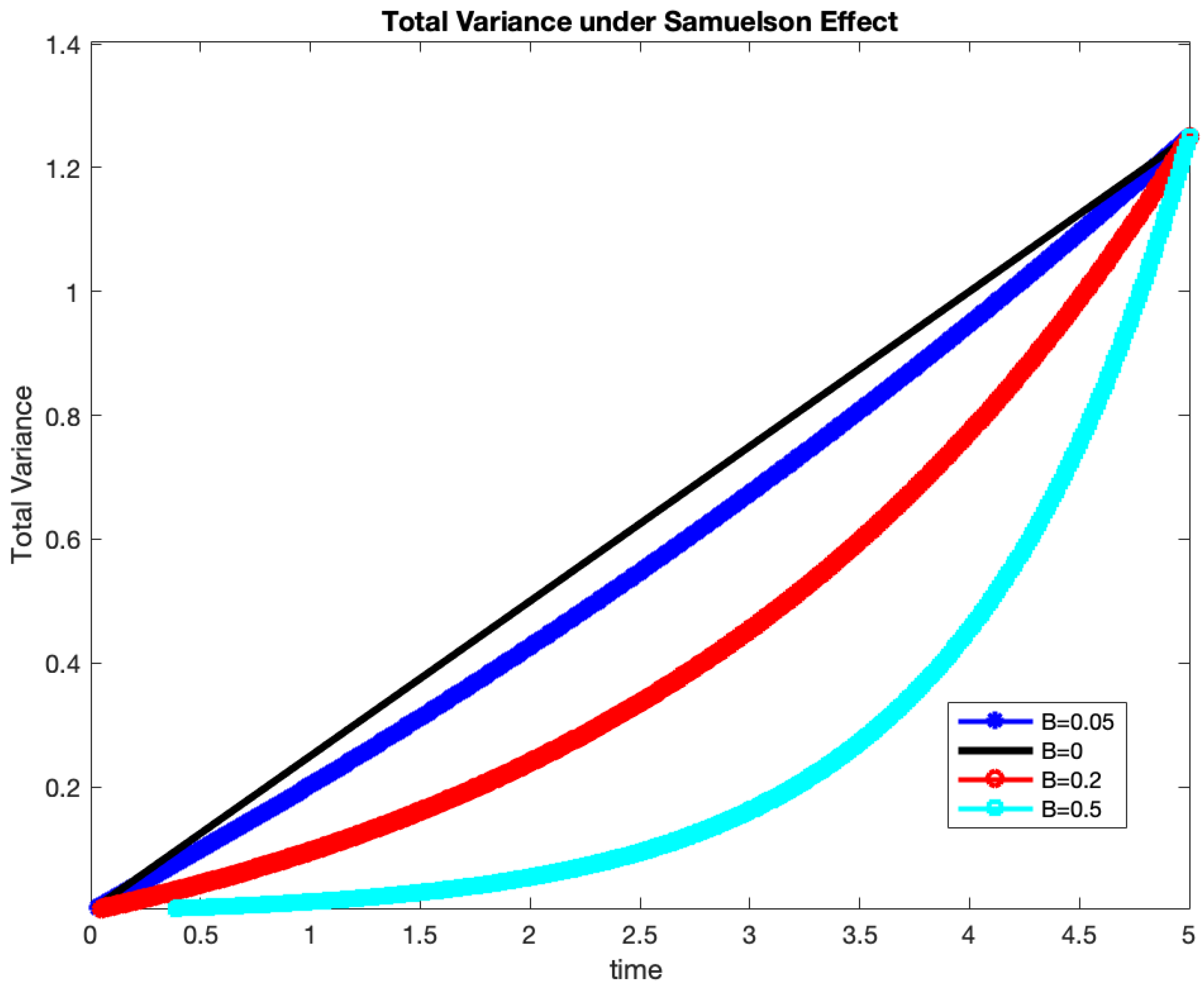
Introducing time-dependent instantaneous variance can be interpreted as a non-uniform clock: we treat the total realized variance as “time.” Under Samuelson, the clock ticks slowly regarding the distant future and accelerates as we approach expiry. Figure 1 below depicts this concept. The example employs the simplest model (1) for instantaneous variance (hence, ${\sigma }_{\infty }=0$). We compute the total variance of a futures contract with maturity of five years and plot it as a function of time t. The market-implied volatility of the future is set at ${\sigma }_{imp}=50\%$. We examine several decay values: $B=0,0.05,0.2,0.5$, from no Samuelson to slight, moderate, and very strong decay. In every instance, the total realized variance from $t=0$ to expiry T must correspond to the market-implied variance $I=0.5^2\times 5=1.25$, while the path used to achieve this is contingent upon B. For a strong Samuelson with $B=0.5$, about $60\%$ of the total variance occurs in the last year of the contract’s duration.

Our calibration technique involves capturing the instantaneous variance by computing variances of returns of nearby contracts. The closest research to our paper in the existing literature is the mentioned paper by Brooks and Teterin (“BT”) [19]. They also use returns of nearby futures, calculate the their standard deviations, and fit a three-factor parametrization by Nelson and Siegel [20] with exponential decay. However, there are key differences between our approaches. First, BT interpolate futures prices with a Nelson–Siegel curve [20], resulting in a vector of pseudo-price time-series with each time-series corresponding to an exact maturity on every trading day (in industry, such contracts are called constant-maturity contracts and used for risk management purposes). We use the raw prices of nearby future contracts. Even though, as calendar time passes, the time to expiration of nearby futures indeed changes and drifts to zero (Brooks and Teterin [19] called it “the maturity drift problem”), we deliver convincing results of the volatility–maturity relationship using raw prices.

Second, BT employ only 12 nearby contracts, while we include all available information, 60 contracts. BT do not account for seasonality when considering term structure of NG volatility. Our data includes crisis period of Spring 2020, which is quite an interesting period to test models.

Third, the models and the targets of the fit are different. The NS model [20] for yield curve $y_t\left(\tau \right)$ given by the parametric form

$$y_t\left(\tau \right)={\beta }_{1t}+{\beta }_{2t}\left({\displaystyle \frac{1-e^{-{\lambda }_t\tau }}{{\lambda }_t\tau }}\right)+{\beta }_{3t}\left({\displaystyle \frac{1-e^{-{\lambda }_t\tau }}{{\lambda }_t\tau }}-e^{-{\lambda }_t\tau }\right)$$

(3)

is based on the forward yield curve; see [34]:

$$f_t\left(\tau \right)={\beta }_{1t}+{\beta }_{2t}{e}^{-{\lambda }_t\tau }+{\beta }_{3t}{\lambda }_t{e}^{-{\lambda }_t\tau }$$

(4)

BT use (3) to model average volatility ${\sigma }_t\left(\tau \right)$ of a synthetic forward contract with constant maturity $\tau$ (in months). We fit instantaneous variance employing a representation (2) similar to (4) but with two exponential decays. The primary input in the model, which determines the Samuelson strength, is the exponential decay parameter B. In BT’s methodology, the exponential decay parameter ${\lambda }_t$ is constant during the initial fitting stages, while the key parameter reflecting the Samuelson effect is represented by the slope of the volatility-term structure ${\beta }_{2t}$.

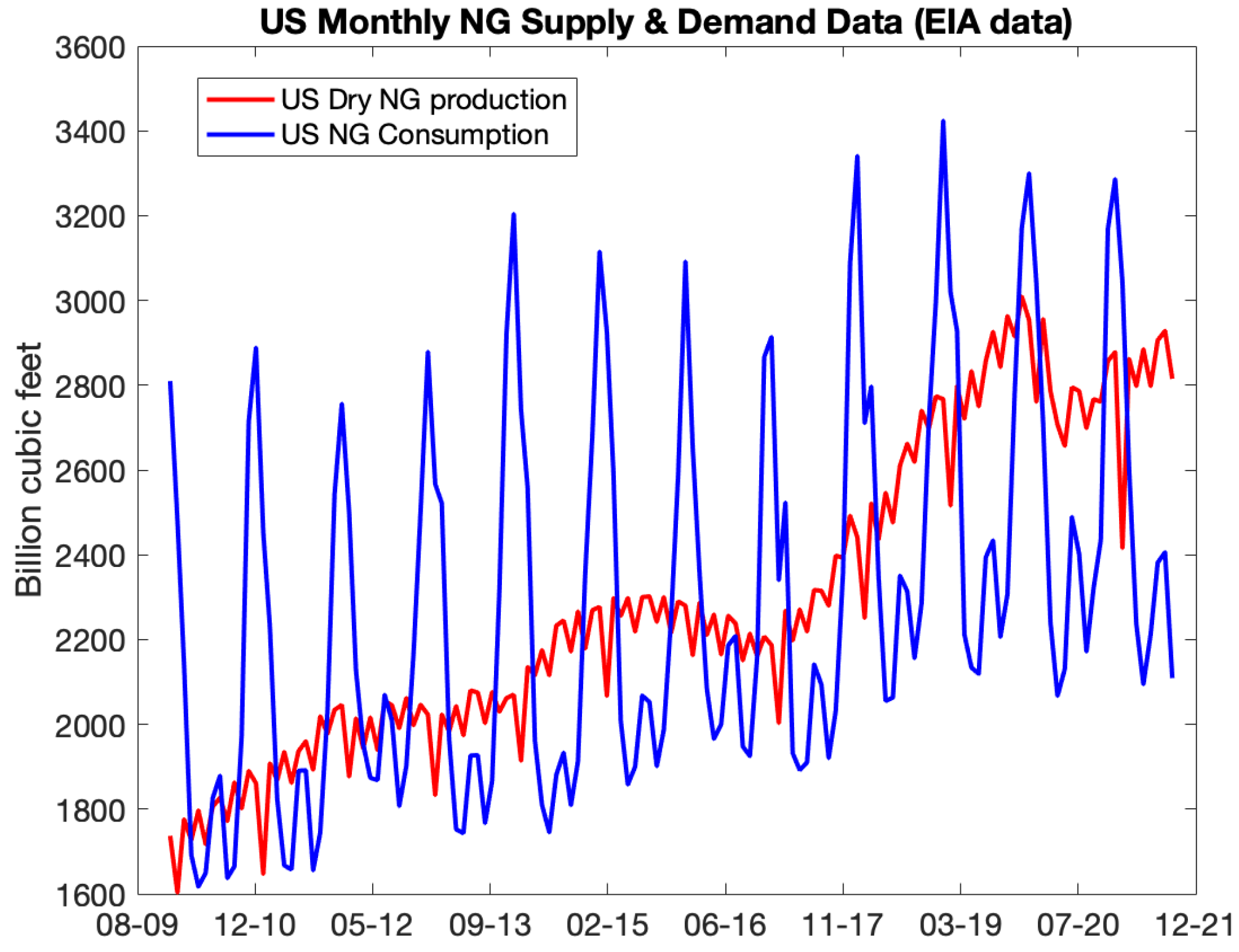
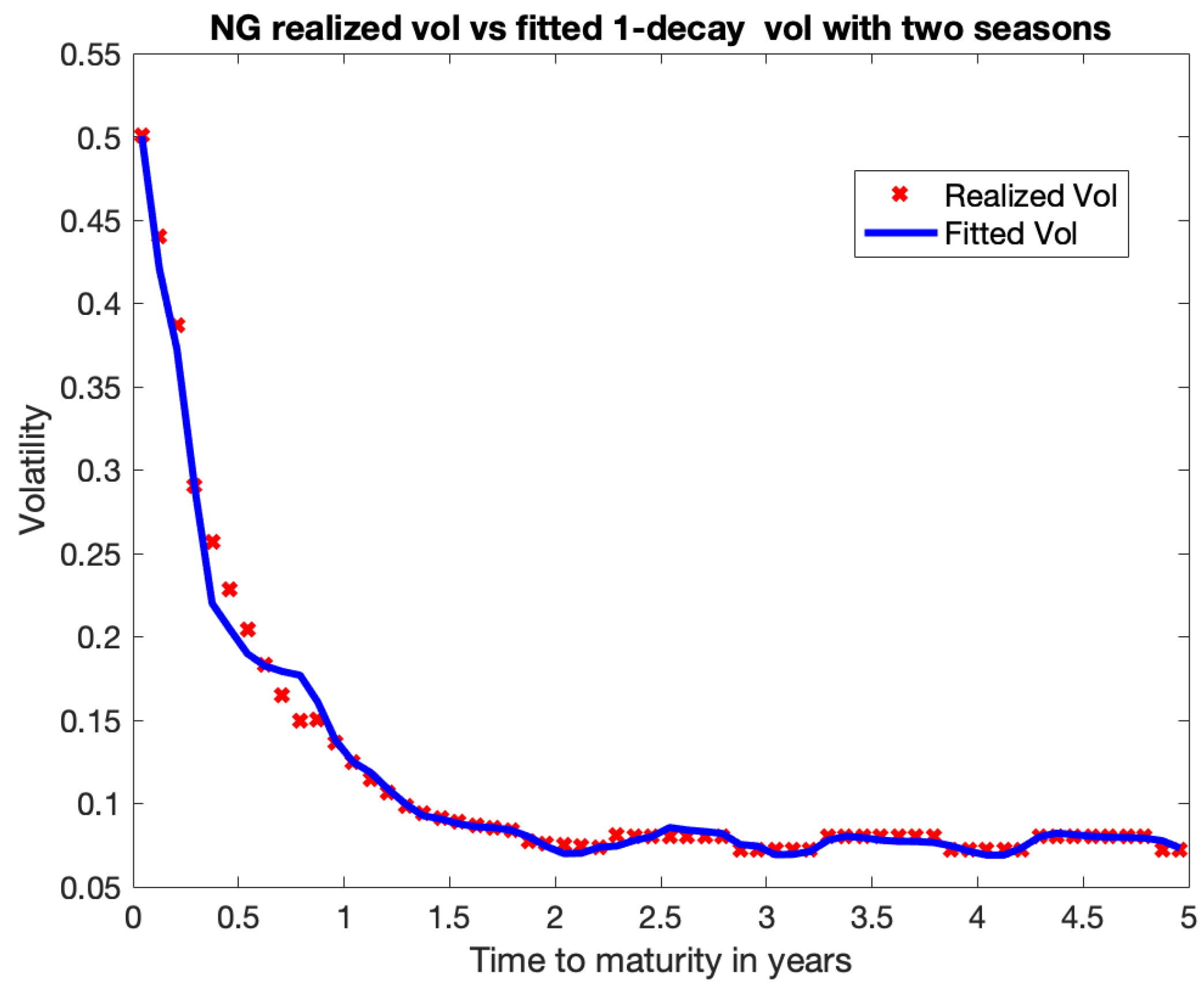
We generalize the calibration methodology to seasonal commodities such as natural gas. The natural gas term structure is defined by seasonality. Natural gas storage is a vital part of the natural gas delivery system and helps to balance supply and demand. During the winter season, from November to March (withdrawal season), gas consumption peaks as a result of increased heating demand. During the summer season, from April to October (injection season), gas demand decreases while production continues. Because of this, we fitted Samuelson independently after dividing the data for nearby futures into two periods: winter and summer. Due to our reliance on data regarding nearby contracts, this separation prevented us from combining returns from different periods, such as March and April. Consequently, we are compelled to employ only two months of the observation period data. Although the fitting findings were favorable, with errors remaining predominantly inside the statistical margin, the outcomes lack consistent stability due to the short observation period. Incorporating additional seasons might exacerbate the existing problems.

The next target is to find the methodology for the Samuelson effect for a more complicated case of seasonal commodities, in particular electricity futures. Electricity has always been the most fascinating commodity to study due to non-storability (at least in meaningful quantities), resulting in very high volatility and abundance of extreme events. Because supply and demand have to be in equilibrium at all times, the electricity seasonality is more refined than for any other seasonal commodity. Each hour in each weekday and month has its own pattern and can be traded separately. Therefore, using only two seasons would not be enough, and we need to come up with a more granular seasonal model. The previous seasonal model for natural gas implies that ${\sigma }_0$ is roughly the same for months in the same season, and the Samuelson parameters B, ${\sigma }_{\infty }$, and $\beta$ are different for winter and summer months. Since we used only two months of nearby futures data, we were catching the Samuelson effect locally, at that particular period of time. The goal is to come up with a methodology that is applicable to long-term deals, such as popular power purchase agreements (“PPA”), which become increasingly more popular in view of growing use of renewable energy. We use the same model for the instantaneous variance (2), with $\beta =0$; however, there are several differences between the two approaches. Firstly, we assume that the normalization constant ${\sigma }_0$ depends on a month in a year, and the Samuelson parameters B and ${\sigma }_{\infty }$ are the same for all the months. We consider only the 1-decay model with $\beta =0$. 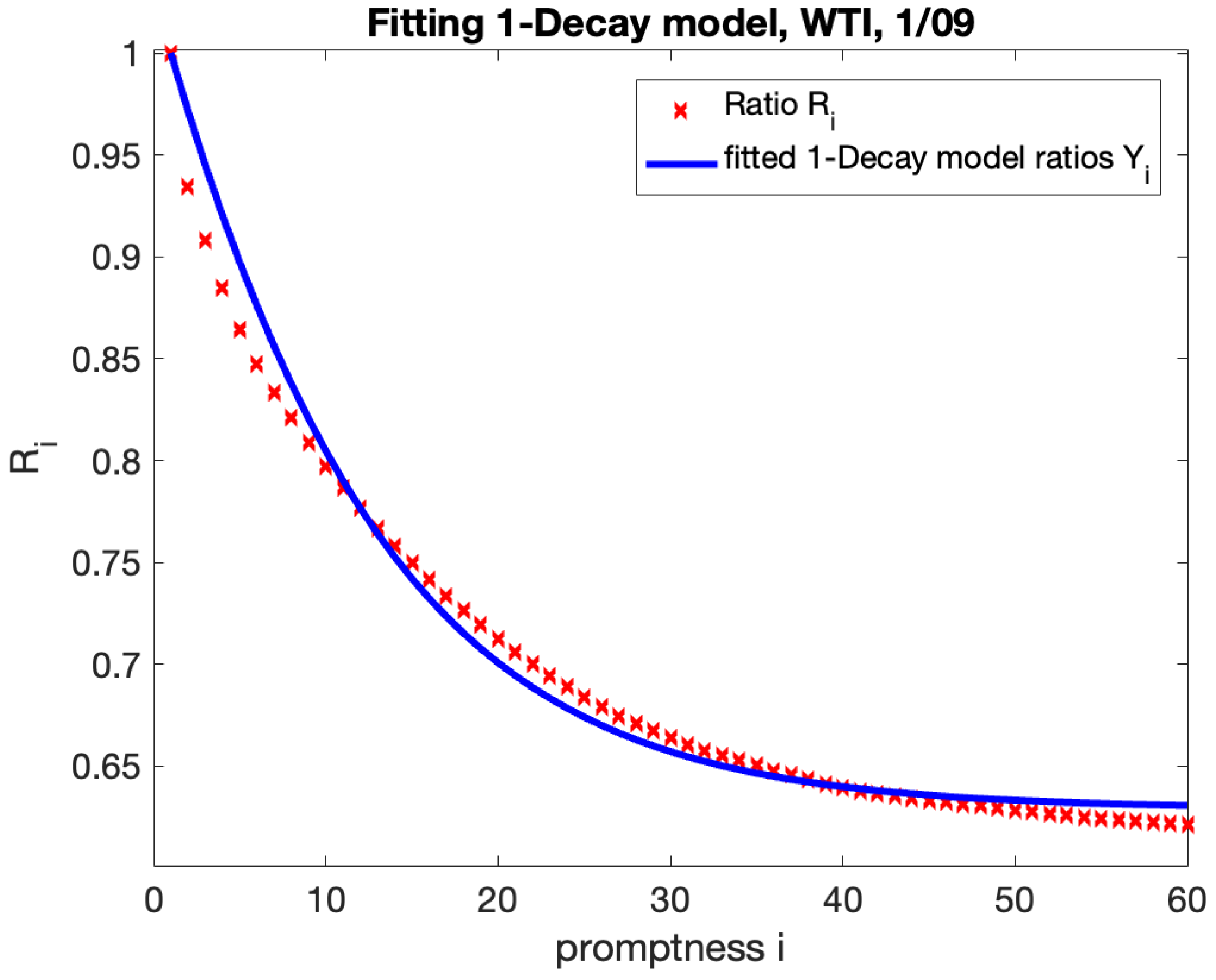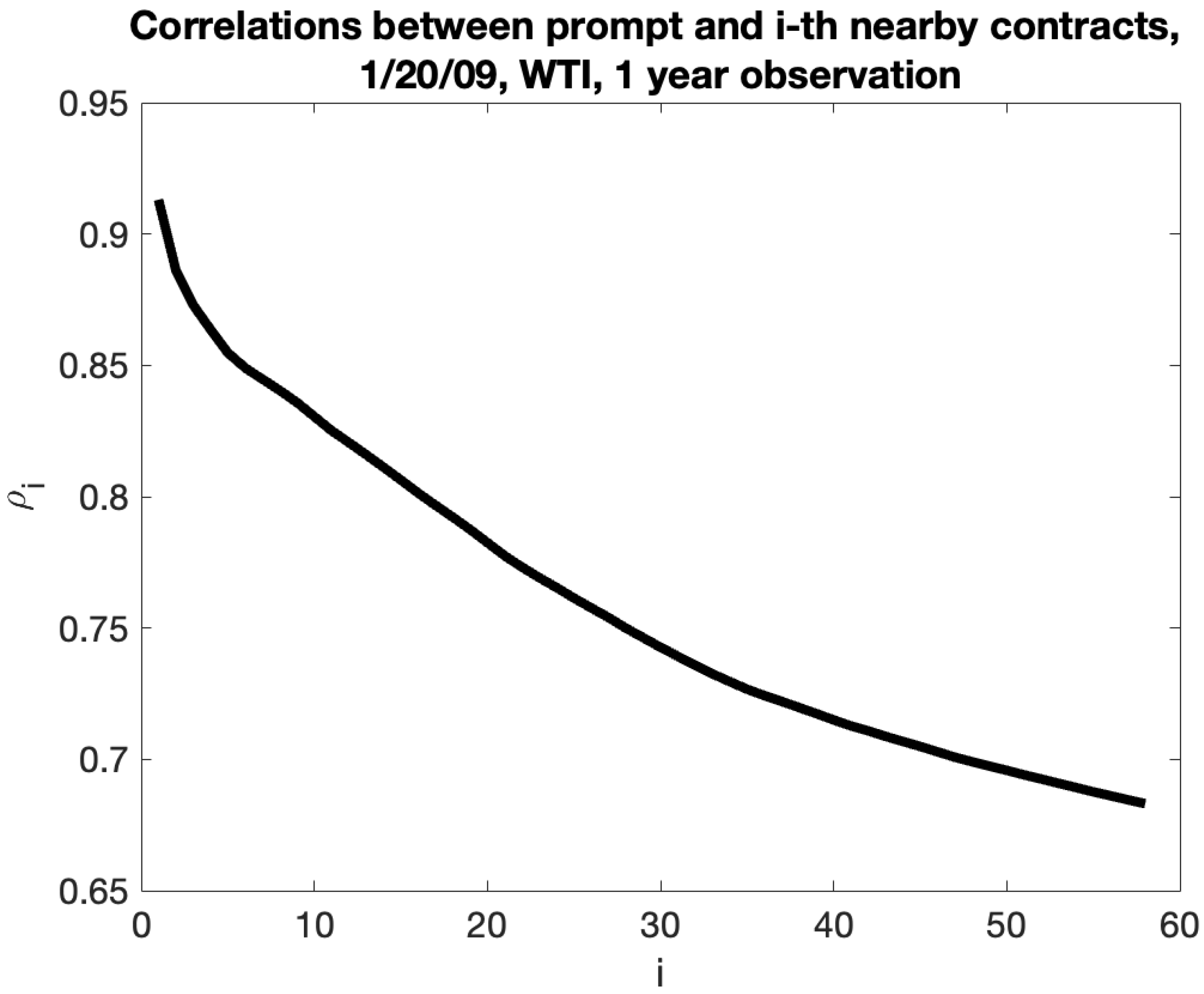Secondly, we use the real futures data and calculate the realized variance regarding a one-year observation period. As in the previous model, we calculate the ratios of variances, but now we use the variances of the same calendar month. We average the ratios for 12 moving observation periods and fit the model. The results are stable.

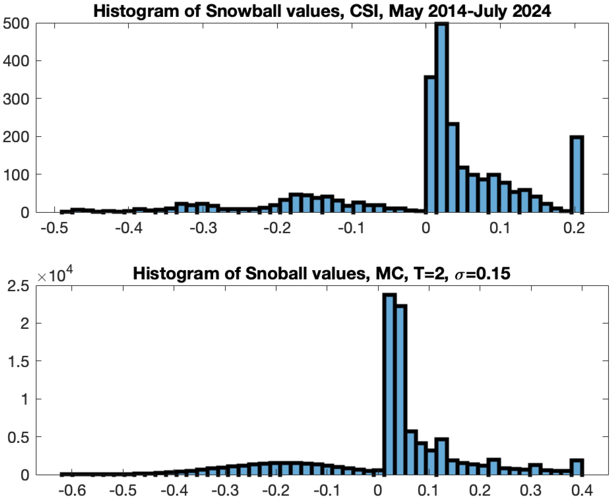
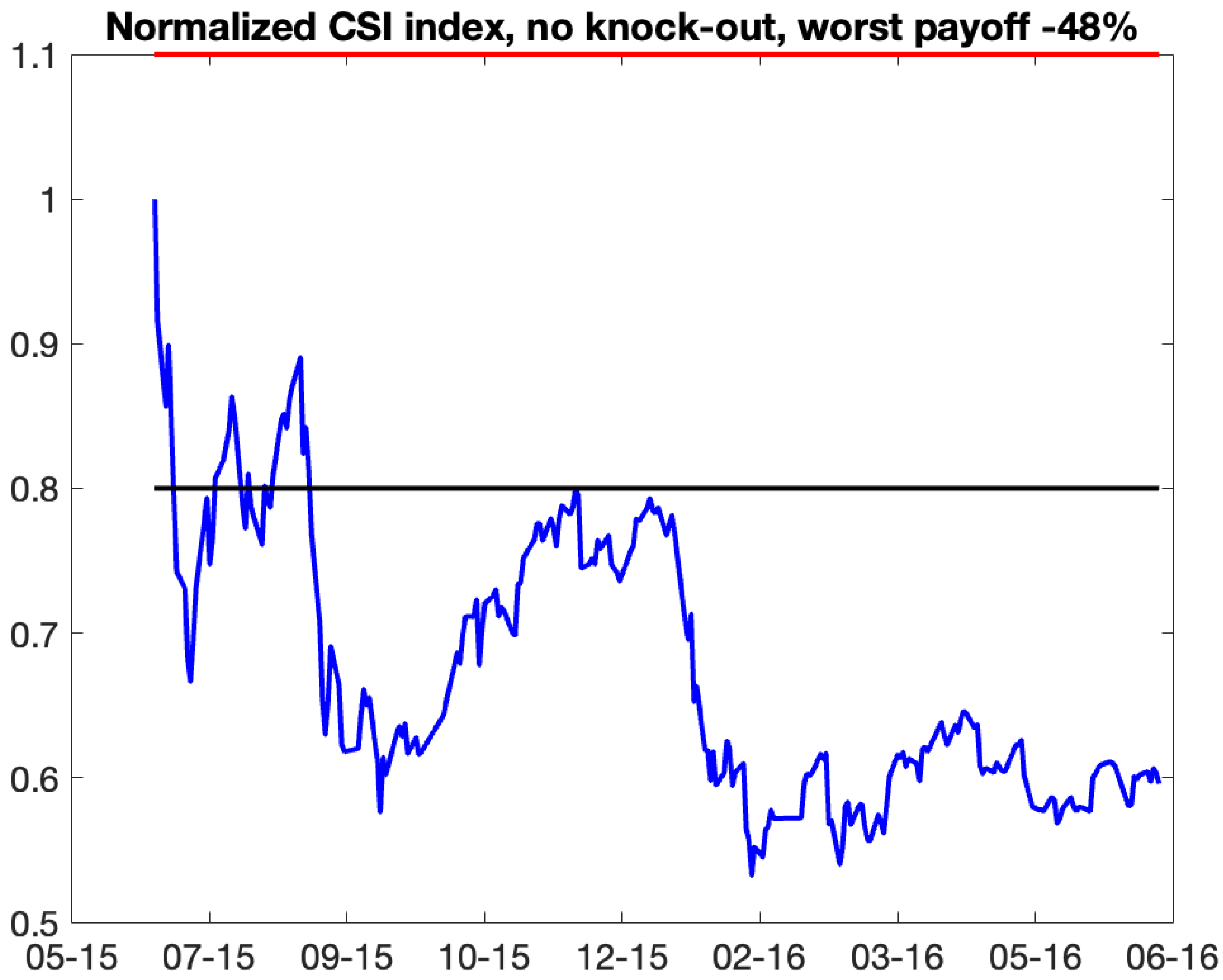
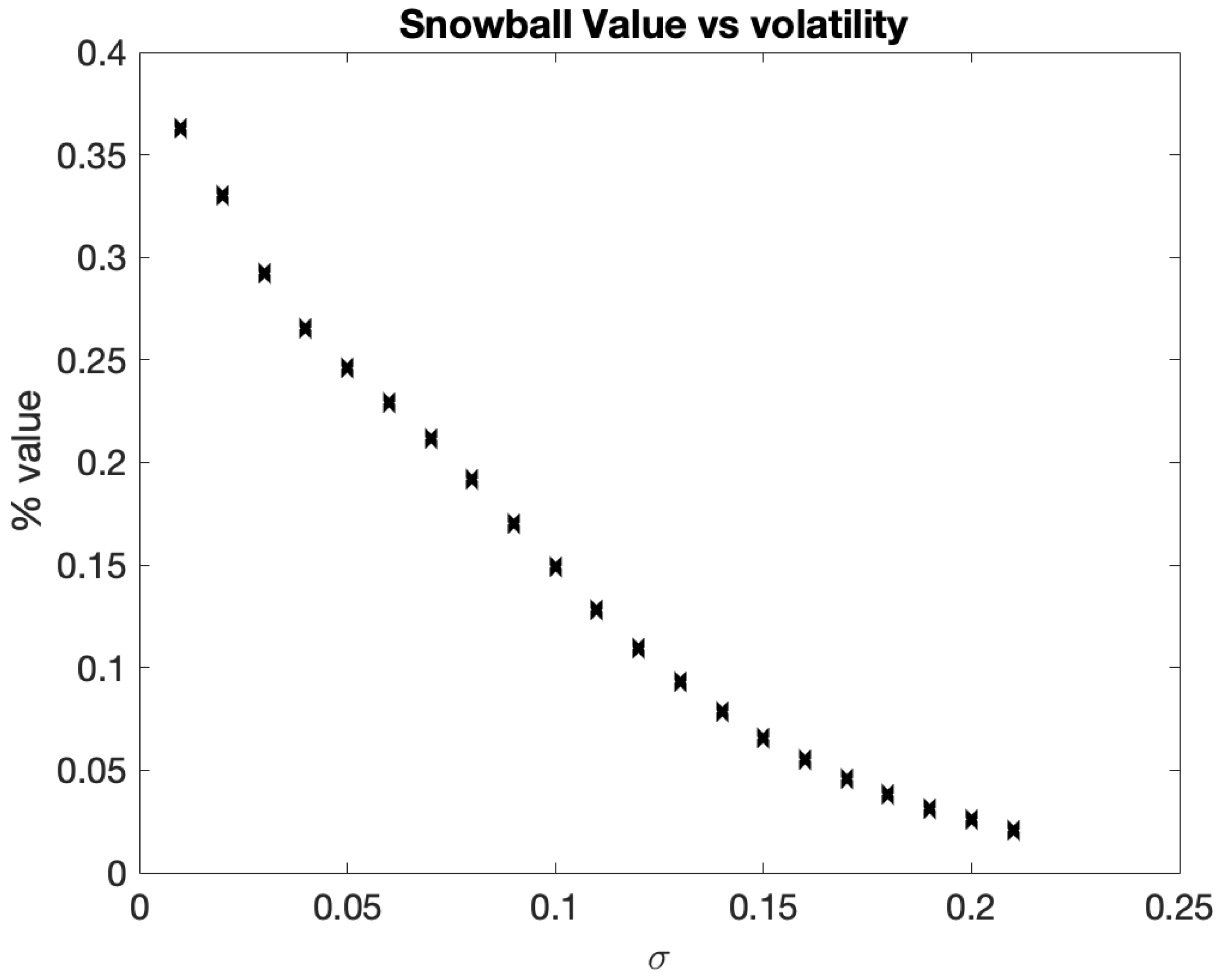
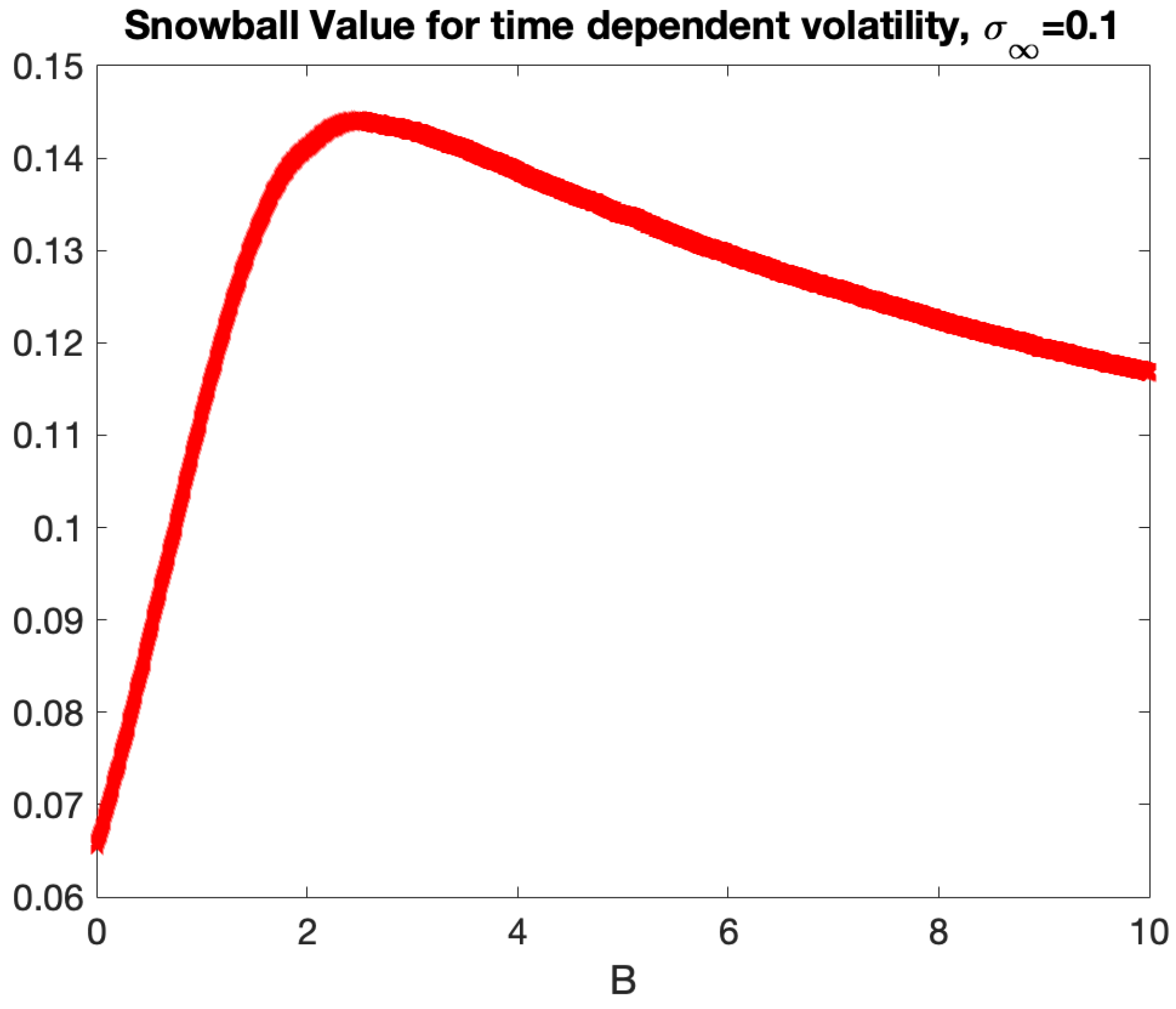
We demonstrate how the Samuelson effect can be used for commodity derivatives. Firstly, we outline the evaluation of early expiration options, such as swaptions. Secondly, we demonstrate how the calibrated model of the instantaneous variance can be used to extrapolate implied volatilities, which is crucially important in the evaluation of PPAs. Furthermore, we discovered an intriguing application of the Samuelson effect to a popular auto-callable equity derivative, the snowball; see [35]. The term ”snowball” describes an investor’s potential for profit accumulation. A snowball is type of auto-callable structure with two barriers: knock-out and knock-in set up as percentages of the initial price. The longer the investor retains an income certificate, the greater the profit, provided the underlying does not drop precipitously. Consequently, the payment of the snowball is contingent upon the realized variance of the underlying asset and the rate of its accumulation. Issuing auto-callable derivatives on assets influenced by the Samuelson effect can be beneficial as initial low volatility may extend the duration of the asset remaining within barriers, hence yielding greater profit. Furthermore, we identified that, based on the structure of a snowball, keeping the realized variance constant, there is an optimal rate of variance growth that yields maximal profit.

We will now delineate the subsequent sections of the article. Section 2 describes the calibration methodology, including generalization for seasonal commodities such as natural gas and electricity. Section 3 examines the results of the calibration employing 15 years of data for WTI, Brent, natural gas, and ERCOT North Hub electricity futures. We discuss the optimal choice in observation period, the model selection, and the analytics of the statistical errors to assess the goodness-of-fit. In Section 4, we demonstrate the application of the calibrated model of instantaneous variance for the evaluation of commodity derivatives, including swaptions, power purchase agreements (PPAs), and auto-callable derivatives linked to commodity futures. The main results of the article are presented in Section 5, which also details the direction of future research. Some specifics are provided in Appendix A and Appendix B.

2. Methodology for Samuelson Effect Calibration

This section is dedicated to providing an in-depth description of the Samuelson effect calibration process.

2.1. Data Selection and Calculation of Normalized Ratios

We start by going over the data selection process in depth, covering the features and scope of the data sample.

A variety of data types can be employed to calibrate a specific Samuelson form.

• Market-implied at-the-money volatilities.
• Historically realized volatilities of futures contract returns with expirations $T_i,i=1,2\dots n$, calculated at time period $[t_a,t_b],t_b<T_1$, $T_1<T_2\dots <T_n$.
• Historically realized volatilities of returns of nearby contracts.

In the last option, we employ the concept of “promptness” of a contract instead of specific contracts. The first nearby contract, referred to as the prompt, is the closest future contract that is accessible at time t and has the shortest duration to expiration. The second nearby contract is the next accessible contract, etc. The second neighboring contract takes over as the first one when the first one expires and so on. The Samuelson effect should result in lower volatility for futures with farther-off expirations.

Employing the first choice—market-implied volatilities, which include forward-looking information—offers clear benefits. The liquidity of options on futures beyond one year is, nevertheless, inadequate. The example below in Figure 2 does not show an immediate decrease in implied volatility, possibly due to local market disruptions. However, historical realized volatilities reveal that realized volatilities usually decrease with expiration $T_i$. Figure 2 presents a comparison.

Since our approach is based on modeling instantaneous variance, the second source of data would involve integration to arrive to realized variance. Therefore, we choose to employ nearby contracts to capture the “true” instantaneous volatility. Thus, the third approach—the volatilities of returns of nearby contracts—is the data of choice for our analysis, with the exception that, for electricity, we had to resort to the second option. Our investigation includes 15 years of data for WTI, Brent, and natural gas futures obtained from the Barchart website. To calibrate Samuelson for electricity futures, we utilize eight years of historical data on electricity futures from Argus Media.

In order to eliminate the impact of volatility level and make the statistics comparable, we normalize the variances of the i-th nearby contract by the variance of the first nearby contract:

$$R_i^2={\displaystyle \frac{{\sigma }_i^2}{{\sigma }_1^2}}$$

(5)

These ratios form the basis of the calibration procedure. Joarder [36] examined the statistical properties of the product and ratio of two correlated chi-squared random variables. The findings of the research can be used to calculate the statistical errors of the ratios. Appendix A offers the specifics.

2.2. Calibration Procedures

We establish a set of model parameter $\mathrm{\Theta }$:

$$\mathrm{\Theta }=\{B,{\sigma }_{\infty },\beta \}$$

and model ratios $Y{\left(\mathrm{\Theta }\right)}_i$ that are inferred from the instantaneous variance’s form (2):

$$Y{\left(\mathrm{\Theta }\right)}_i=\sqrt{{\displaystyle \frac{e^{-2B(T_i-t)}+{\sigma }_{\infty }^2{e}^{-2b(T_i-t)}}{e^{-2B(T_1-t)}+{\sigma }_{\infty }^2{e}^{-2b(T_1-t))}}}}$$

(6)

where $T_i$ and $T_1$ are times to maturity (in years) of the i-th and the first nearby contracts correspondingly.

The traditional model calibration procedure follows the conventional approach for identifying the model parameters that optimally align with historical data. First, we choose an observation period $[t_a,t_b]$ and construct series of nearby contracts $F_m^{\left(i\right)}$ of historical settlement prices observed daily at $t_m\in [t_a,t_b]$ and $m=1,2,\dots ,M$, $t_1=t_a$, $t_m=t_b$; $i=1,\dots N$, where N is the number of observed contracts. Usually, N = 60. For non-seasonal commodities, we employ observation periods of two and twelve months, while, for seasonal commodities, we utilize a two-month timeframe. A two-month observation period typically comprises M = 44 observations (days), whereas a twelve-month observation period has M = 252 days. We compute log-returns

$${\displaystyle \frac{ln(F_m^{\left(i\right)}/F_{m-1}^{\left(i\right)})}{{(t_m-t_{m-1})}^{1/2}}}$$

(7)

We next compute realized variances of returns and document the previously established ratios. A constrained minimization of the total error determines the optimal set of model parameters

$$E\left(\mathrm{\Theta }\right)=\sqrt{\sum _{i=2}^N{\displaystyle \frac{{[Y{\left(\mathrm{\Theta }\right)}_i-R_i]}^2}{N-1}}}$$

(8)

where $Y{\left(\mathrm{\Theta }\right)}_i$ are the model ratios given by (6). We assume that decay occurs mostly due to increase in $T_i$ and cancel out the normalization constant ${\sigma }_0$. The specific choices in parameters $\mathrm{\Theta }$ and constraints are revealed in each case.

The primary challenge of the minimization problem is the possibility of various solutions because of the way parameters influence the ratios: an increase in long-term volatility ${\sigma }_{\infty }$ weakens the decay, whereas a higher B drives ratios to decay more quickly. We should stay away from certain areas of the parameter space where slight adjustments to ratios result in significant changes to decay or long-term volatility. Several contour plots of the 12-month ratio $Y_{12}$ for the scenario where the long-term decay $\beta =0$ are shown in the following Figure 3 to demonstrate this.

The model with two decays, B and $\beta$, will be referred to as the 2-decay model, whereas the model with $\beta =0$ will be called the 1-decay model. Only in times of crisis, when Samuelson is very strong, do we need to use a more intricate 2-decay model. The following section will provide examples.

2.3. Samuelson Effect for Seasonal Commodities

To accommodate Samuelson, the previous approach must be modified for seasonal commodities such as electricity, natural gas, heating oil, and gasoline. Our first emphasis is on natural gas, one of the most significant and “physical” commodities. The first seasonal model for natural gas assumes that ${\sigma }_0$ is roughly the same throughout months within the same season, and the Samuelson parameters B, ${\sigma }_{\infty }$, and $\beta$ are different for winter and summer months.

The subsequent objective was to identify the methodology for the Samuelson effect in a more complex scenario involving seasonal commodities, specifically electricity futures. Seasonality is more nuanced for electricity than for any other seasonal commodity. Every hour of each weekday and month exhibits a distinct pattern and can be traded independently. Consequently, relying solely on two seasons is insufficient; we must develop a more detailed seasonal model. We employ the identical model for the instantaneous variance (2) with $\beta =0$ while positing that the normalization constant ${\sigma }_0$ is contingent upon the month of the year, while the Samuelson parameters B and ${\sigma }_{\infty }$ remain constant across all months. We utilize actual futures data to compute the realized variance over a one-year observation period. Similar to the prior model, we compute the ratios of variances; however, we now utilize the variances from the same calendar month. We compute the average ratios over a 12-month period, adjusting the observation timeframe, and subsequently fit the model. The results are stable.

2.3.1. Natural Gas

A typical monthly supply–demand chart for natural gas (NG) based on EIA data is shown in Figure 4. This type of chart can be found in many natural gas market references, such as [33]. Particularly during the winter, storage is essential to closing the gap between supply and demand.

There are significant winter peaks in demand because of the cold weather, and milder summer peaks because of rising power use. Demand is cyclical, which causes seasonal patterns in prices and volatility. This makes a volatility-term structure a superposition of decay with time to expiration and seasonal shape. An illustration of implied NG volatility can be found in Figure 5.

Based on the data and the widely accepted description of natural gas storage seasons, we also choose to divide the Samuelson data into two periods: a summer (injection) season that runs from April to October and a winter (withdrawal) season that runs from November to March.

Because of this division, we are unable to combine returns from various seasons, such March and April. Using an observation period of just one month is an easy fix. Fitting results are not convincing though because variance measured on (about) 22 data points is extremely noisy. As a result, we carefully chose a two-month observation period. For example, in September and October, we observe first nearby futures prices from different seasons; therefore, this period does not work. There are even more issues if we use additional months in the observation period, such as four or six, because we would have to leave out more combinations. Therefore, we decide to employ two months for the study time.

Using a similar process to that used for oil, mutatis mutandis, we fit a seasonal Samuelson independently.

2.3.2. Electricity

Electricity has consistently been the most intriguing commodity to examine due to its non-storability (at least currently, in significant quantities), resulting in considerable volatility and a prevalence of extreme events. Due to the necessity for supply and demand to be in equilibrium at all times, electricity seasonality is more nuanced than any other seasonal commodity regarding both prices and volatilities.

Given this behavior, we formulate the subsequent assumptions regarding the dynamics of instantaneous variance (2).

• We presume $\beta =0$.
• The parameters B and ${\sigma }_{\infty }$ remain constant throughout the year.
• The normalization constant ${\sigma }_0$ solely dependent on the month of the year and remains constant throughout all years.

We will now delineate the process for calibrating the Samuelson parameters B and ${\sigma }_{\infty }$ using historical data of futures prices seen over a one-year period. For instance, we consider the year 2022 as the targeted observation period. We select the initial contract as the one we monitored until its expiration throughout the observation period, specifically January 2023.

We adhere to the subsequent steps:

• Record prices for the chosen contract for about one year prior to the expiration. In this particular instance, observations commence at time $t_1$, 1 January 2022, and continue until the contract’s expiration at $t_2=T_1$, contingent upon the market (for example, ERCOT futures expire on the second to last business day of the month prior to the contract month). The observation period is defined as $[t_1,t_2]$.
• Calculate log-returns and their standard deviation ${\sigma }_{real}^{Jan23}$. This represents the realized volatility of the first contract.
• Simultaneously compute the log-returns of further forward contracts, including 23 February, 23 April, and extending four years forward to 26 December, with the identical observation period $[t_1,t_2]$, and determine the standard deviations of their log-returns. Document 48 realized volatilities.
• Calculate ratios by dividing the volatility of each month and year by the volatility of the same month in the previous year:

  $$R(t_1,t_2,T_i+1,T_i)={\displaystyle \frac{{\sigma }_{real}^{i,yr+1}}{{\sigma }_{real}^{i,yr}}},i=1,...36$$
• Record 36 ratios, which are functions of $T_i-t_1$ and $T_i-t_2$, only assuming the normalization constant ${\sigma }_0$.

Subsequently, replicate the aforementioned steps 1–4, commencing with 23 February, while advancing the observation term by one month, initiating from 1 February 2022, until the contract’s expiration. The approach yields an additional set of 36 ratios. Select 23 March and continue until December 2023. Consequently, we shall obtain 12 sets of 36 ratios. Observe that the time periods $T_i-t_1$ and $T_i-t_2$ are approximately same across all sets.

$$T_i-t_2\approx {\displaystyle \frac{i-1}{12}},T_i-t_1\approx {\displaystyle \frac{i-1}{12}}+1,i=1,2...,36.$$

Given that they rely solely on times rather than the month of the year, we can average each promptness i across 12 sets to determine the optimal parameters B and ${\sigma }_{\infty }$ that encapsulate the Samuelson effect.

Our objective is to develop a methodology suited to long-term agreements, such as prevalent power purchase agreements (PPAs). Consequently, we have opted to examine a global pattern of volatility-term structure rather than a more detailed seasonal decay as conducted in our analysis of natural gas.

We will now describe the outcomes of the calibration tasks.

3. Results

This section examines the calibration results using 15 years of data for WTI, Brent, and natural gas futures, along with the selection of the observation period and model (1-decay versus 2-decay). A 12-month observation period for WTI and Brent, a 2-month duration for natural gas, and a first-order decay model tend to be efficacious. During crises, when the Samuelson effect is significant, it is essential to employ a more refined 2-decay model. We provide analytics for statistical errors on normalized variances to provide a baseline for the calibration results and assess the error relative to the lower bound of the statistical error for WTI and Brent. To achieve this, we utilize a rolling window of 12 months (252-day interval). We conclude that, for a majority of times, excluding the crisis years of 2009 and 2020, the model aligns effectively with the data within the bounds of statistical error.

We provide the calibration results of the Samuelson effect for electricity futures at a major trading hub, namely ERCOT North in Texas. We begin with a review of the descriptive statistics of the log-returns for WTI, Brent, and natural gas futures.

3.1. Descriptive Statistics

We meticulously examine the returns of the first four nearby contracts. We label the first nearby contract series of WTI as WTI1, the second nearby as WTI2, and so forth. Correspondingly, we assign the names of the contracts Brent1 to Brent4 for Brent Oil futures and NG1 to NG4 for natural gas. The findings are displayed in

Table 1. Descriptive statistics of WTI, Brent, and natural gas return series.

Series	Count	Mean	Std. Dev.	Median	Minimum	Maximum	Skewness	Kurtosis
Dataset 1: WTI (Data Period: 21 April 2006–9 June 2021)
WTI1	3813	$0.0000$	$0.0246$	$0.0004$	$-0.3008$	$0.2239$	$-0.0854$	$21.1870$
WTI2	3813	$-0.0002$	$0.0229$	$0.0006$	$-0.3858$	$0.2182$	$-1.3883$	$32.2534$
WTI3	3813	$-0.0001$	$0.0213$	$0.0006$	$-0.2461$	$0.2002$	$-0.5281$	$13.6756$
WTI4	3813	$-0.0000$	$0.0204$	$0.0007$	$-0.2209$	$0.1858$	$-0.4155$	$10.5347$
Dataset 2: Brent (Data Period: 16 June 2006–9 June 2021)
Brent1	3869	$0.0001$	$0.0211$	$0.0005$	$-0.2798$	$0.1908$	$-0.4527$	$14.8710$
Brent2	3869	$-0.0000$	$0.0202$	$0.0006$	$-0.2338$	$0.1352$	$-0.3946$	$9.6590$
Brent3	3869	$-0.0000$	$0.0195$	$0.0006$	$-0.2054$	$0.1278$	$-0.3646$	$7.6978$
Brent4	3869	$-0.0000$	$0.0189$	$0.0006$	$-0.1865$	$0.1240$	$-0.3429$	$6.7611$
Dataset 3: Natural Gas (Data Period: 29 June 2006–9 June 2021)
NG1	3772	$-0.0011$	$0.0266$	$-0.0009$	$-0.1805$	$0.1651$	$0.1735$	$2.6956$
NG2	3772	$-0.0012$	$0.0238$	$-0.0011$	$-0.1918$	$0.1664$	$0.1204$	$3.0882$
NG3	3772	$-0.0010$	$0.0216$	$-0.0008$	$-0.2021$	$0.1713$	$0.0427$	$4.3136$
NG4	3772	$-0.0008$	$0.0199$	$-0.0006$	$-0.2180$	$0.1863$	$0.0078$	$7.2988$

. The standard deviations are daily and increase as maturity approaches. We opt to exclude the negative price date for WTI contracts to prevent complications in the calculation of log-returns.

3.2. Results of Samuelson Calibration, WTI, Brent, and Natural Gas

We conducted the fitting technique multiple times throughout a designated observation period for WTI, Brent Oil, and natural gas.

Table 2. Examples of WTI calibration results.

${\mathit{t}}_{\mathit{a}}$	${\mathit{t}}_{\mathit{b}}$	B	${\mathit{\sigma }}_{\mathbf{\infty }}$	RMSE
12/21/11	12/19/12	0.2937	0.5678	0.0014
11/19/12	11/20/13	0.4611	0.4953	0.0003
10/23/13	10/21/14	0.6627	0.4663	0.0004
9/23/14	9/22/15	0.4803	0.4856	0.0006
8/21/15	8/22/16	0.4624	0.5773	0.0063
7/21/16	7/20/17	0.3959	0.5966	0.0007
6/21/17	6/20/18	0.4864	0.6964	0.0008
5/23/18	5/21/19	0.2980	0.6775	0.0008
4/23/19	4/21/20	0.9093	0.3028	0.0252
02/21/19	02/20/20	0.3245	0.4458	0.0018

enumerates the outcomes of WTI calibration throughout a 12-month observation period. The last column denotes the root mean square error (8) computed using the optimal parameters $\mathrm{\Theta }$ of the 1-decay model, scaled by the volatility of the prompt contract.

As an example, we examine the instantaneous volatility of WTI realized during a 12-month observation period, from $t_a$ = 21 February 2019 to $t_b$ = 20 February 2020, with $N=60$. Figure 6 illustrates a fitting graph. The scatter points denote the actual realized volatilities, whereas the line graphs illustrate the fitted model with exponential 1-decay. We calibrated the volatility level by aligning ${\sigma }_0$ with the volatility of the prompt contract.

Table 3. Examples of Brent calibration results utilizing the 1-decay model.

${\mathit{t}}_{\mathit{a}}$	${\mathit{t}}_{\mathit{b}}$	B	${\mathit{\sigma }}_{\mathbf{\infty }}$	RMSE
10/17/12	10/16/13	0.2809	0.4159	0.0013
9/16/13	9/15/14	0.5306	0.4917	0.0004
8/15/14	8/14/15	0.3821	0.4267	0.0026
8/17/15	7/29/16	0.3498	0.5520	0.0012
7/1/16	6/30/17	0.3367	0.5495	0.00175
6/1/17	5/31/18	0.3629	0.6853	0.0025
5/1/18	4/30/19	0.2325	0.5715	0.0006
4/1/19	3/31/20	0.4789	0.3813	0.005

presents details on the RMSE errors for Brent over several observation periods.

To examine a seasonal instance of NG, we classify the data into two categories: summer, including April to October, and winter, spanning November to March. We eliminate inter-seasonal combinations and thereafter adjust the parameters for each season accordingly. Due to seasonality, we can only employ two months of return data. As a result, the assessments of true instantaneous volatility demonstrate increased noise. The model may not correspond as accurately as it does with WTI; however, it sufficiently represents seasonal fluctuations. The subsequent

Table 4. Natural gas calibration results: “W” denotes winter, whereas “S” signifies summer.

${\mathit{t}}_{\mathit{b}}$	B W	${\mathit{\sigma }}_{\mathbf{\infty }}$ W	B S	${\mathit{\sigma }}_{\mathbf{\infty }}$ S	RMSE
$11/24/08$	$0.721$	$0.434$	$0.660$	$0.487$	$0.0068$
$12/29/09$	$0.837$	$0.318$	$0.670$	$0.349$	$0.0118$
$12/28/10$	$0.913$	$0.265$	$0.865$	$0.294$	$0.0118$
$12/28/11$	$0.675$	$0.371$	$0.556$	$0.406$	$0.0071$
$11/28/12$	$0.647$	$0.375$	$0.526$	$0.416$	$0.006$
$11/26/13$	$0.486$	$0.327$	$0.447$	$0.368$	$0.0038$
$5/29/18$	$1.049$	$0.283$	$0.979$	$0.360$	$0.0038$
$12/27/19$	$1.586$	$0.137$	$1.581$	$0.181$	$0.0083$
$4/28/20$	$2.515$	$0.085$	$1.536$	$0.179$	$0.0141$

presents the calibration results for NG across various time periods.

Figure 7 illustrates the actual NG volatility compared to the fitted volatility with a 1-decay model. The realized volatility is calculated using the log-returns of natural gas for the period from 30 October 2019 to 27 December 2019.

3.3. Results of Samuelson Calibration for Electricity Futures

ERCOT Markets

We begin with the ERCOT (Electric Reliability Council of Texas) market, which is very unique and widely known for its significant price volatility. It is an energy-only market, which means generators are only compensated for the energy they provide to the grid, unlike other markets that also compensate for capacity availability. ERCOT added another component to wholesale prices in 2015, a scarcity adder. This scarcity adder represents the value of additional resources to grid reliability. Further, ERCOT’s electricity system operates within Texas and is not subject to federal control by the Federal Energy Regulatory Commission (FERC). ERCOT’s transmission grid is solely contained inside the state of Texas and is not linked to other states’ networks. These two facts make ERCOT an “energy island”.

ERCOT’s electricity prices are volatile due to several factors, including Texas’s unique weather patterns, its independent electrical grid, increasing demand, and the integration of intermittent renewable energy sources such as wind and solar. In February 2021, extremely low temperatures during Winter Storm Uri forced significant generation equipment to freeze, leading to prolonged outages throughout most of Texas. The scarcity adder resulted in elevated ERCOT energy prices, which remained at the price ceiling of USD 9000/MWh for three consecutive days.

Due to the inherent volatility of electricity contracts, we cannot anticipate flawless fitting results, as seen with WTI. The objective is to capture the general decline in volatility by calculating average seasonal ratios, as outlined in Section 2.3.2. The liquidity of energy futures tends to concentrate within the initial two to three years. Consequently, we employed only 24 ratios to calibrate Samuelson.

Figure 8 depicts the realized seasonal ratios in comparison to model ratios determined as of January 2021. This indicates that we computed the average of seasonal ratios for future contracts from January 2020 to December 2020. The fitted Samuelson is strong, which is unsurprising given that the period encompasses the COVID-19 era.

Not all ratios fit as well, but we can usually identify the trend. Figure 9 illustrates a more recent outcome of fitting the average of realized seasonal ratios from 23 June to 24 May.

Table 5. Calibrated Samuelson parameters and ERCOT electricity futures.

Date	B	${\mathit{\sigma }}_{\mathbf{\infty }}$
1/1/18	$0.638$	$0.427$
1/1/19	$0.358$	$0.638$
1/1/20	$3.088$	$0.24$
1/1/21	$0.1702$	$0.15$
1/1/22	$1.522$	$0.146$
1/1/23	$1.548$	$0.325$
1/1/24	$1.218$	$0.493$

shows the results of the Samuelson effect calibration for ERCOT electricity futures. We record the parameters at the start of each year, using an average of 12 seasonal ratios from January to December of the preceding year.

3.4. Finding the Optimal Length of Observation Period

The length of the observation period is essential for volatility calculation and calibration procedures. We provide the subsequent considerations for its selection.

Calculating instantaneous volatility with one-month data from nearby contracts is not adequate as 22 data points might yield a noisy result, leading to a wide confidence interval for the volatility estimate. Therefore, we selected a minimum observation period of two months. A two-month observation period could be a judicious decision, especially during times of crisis. In the spring of 2020, global market volatility was exceptionally high, and conditions were rapidly changing. Employing a two-month period might prove a prudent choice. In a less volatile market, like that of 2019, one may choose a 6-month or 12-month period. A 12-month observation period is optimal as it consistently includes the most liquid December contract. Another rationale for selecting a 12-month observation period is the stability of the fitted parameters.

In conclusion, the selection of a 12-month observation period is our preference and primary case study.

3.5. Model Selection

Upon analyzing the results of the fit across several historical periods, we conclude that the 1-decay model yields fair results in comparison to the 2-decay model in the majority of periods. During stable market conditions, devoid of significant disruptions like the COVID-19 crisis in 2020 or the 2009 financial crisis, it is entirely justifiable to utilize the parsimonious 1-decay model.

Figure 10 illustrates a comparison between the 1-decay exponential model and the 2-decay exponential model. The black line illustrates the graph of the fitted 1-decay exponential model, while the blue line depicts the graph of the 2-decay exponential model. The observed realized volatilities in the tail exhibit a clear decay in long-term volatility. The 2-decay exponential model more accurately reflects the pattern, resulting in an improvement of around 80 basis points in RMSE accuracy, as seen in

Table 6. WTI calibration results: 1 exponential decay model vs. 2 exponential decay model; “1-D” denotes 1-decay model, whereas “2-D” stands for 2-decay model.

	${\mathit{t}}_{\mathit{a}}$	${\mathit{t}}_{\mathit{b}}$	B	${\mathit{\sigma }}_{\mathbf{\infty }}$	b	RMSE
2-D	$11/2008$	$11/2009$	$1.51$	$0.71$	$0.07$	$0.0098$
1-D	$11/2008$	$11/2009$	$0.92$	$0.52$	0	$0.018$

. In 2009 and 2020, the 2-decay model presents far better performance. Similar patterns emerge during periods of market volatility, namely during the crises of 2009 and 2020.

3.6. Statistical Errors on the Normalized Ratios

To evaluate model performance, we developed analytics on the statistical errors of the normalized ratios $R_i^2$ as defined by (5). We consider log-returns (7) of nearby contracts, which have a multivariate normal distribution. The ratio of the variance of the i-nearby contract, normalized by the “true” variance ${\displaystyle \frac{S_i^2}{{\sigma }_i^2}}$, follows a chi-squared distribution with m degrees of freedom, where $m=M-1$ and M equals the number of observations.

Define $U_i={\displaystyle \frac{m{S}_i^2}{{\sigma }_i^2}}$ and $U_1={\displaystyle \frac{m{S}_1^2}{{\sigma }_1^2}}$. The joint distribution of $U_1$ and $U_2$ is referred to as the bivariate chi-squared distribution. Joarder (2009) examined the distribution of the product and the ratio of two correlated chi-squared random variables. We utilized the findings presented in this paper, namely the formulae of the first and second moments of the ratio $W_i={\displaystyle \frac{U_i}{U_1}}$. Specifically, if ${\rho }_i$ denotes the correlation between the log-returns of the i-th nearby contract and the prompt contract, then, for $m>8$ and $-1<{\rho }_i<1$, we have

(i)

$E\left(W_i\right)={\displaystyle \frac{m-2{\rho }_i^2}{m-2}}$, $m>2$

(ii)

$E\left(W_i^2\right)={\displaystyle \frac{1}{(m-2)(m-4)}}\left(24{\rho }_i^4-8(m+2){\rho }_i^2+m(m+2)\right)$, $m>4$

The variance of the ratio W can be computed by

$$Var\left(W_i\right)=E\left(W_i^2\right)-{\left(E\left(W_i\right)\right)}^2$$

As expected, $Var\left(W_i\right)$ vanishes for perfect correlations ${\rho }_i=1$. By substituting $U_i$ and $U_1$ into the equation, we can establish a relationship between $W_i$ and $R_i={\displaystyle \frac{S_i^2}{S_1^2}}$, which is our target variable, the normalized ratio.

$$Var\left({\displaystyle \frac{S_i^2}{S_1^2}}\right)=Var\left(R_i^2\right)={\left({\displaystyle \frac{{\sigma }_i^2}{{\sigma }_1^2}}\right)}^2·Var\left(W_i\right)$$

(9)

Since the “true” variances ${\sigma }_i$ and ${\sigma }_1$ are unknown, it is essential to derive a lower bound using their estimates, $S_i$ and $S_1$. The variances of the normalized ratios (A1) are contingent upon the number of points M, correlations, and Samuelson strength. The ratios decrease with stronger Samuelson and increase with weaker Samuelson. Increasing the number of observations M results in a decline in the ratios. In times of crisis, strong Samuelson decay leads to lower statistical errors, hence compromising model performance. Conversely, during crises and severe Samuelson effects, calendar correlations decrease, leading to contrary outcomes.

We need to find a lower constraint on the total error and verify that the fitting error resides within this statistical error lower bound. For conciseness, the particulars are provided in Appendix A. We present the findings of the comparison between the actual error and the lower bound of the statistical error for WTI and Brent, utilizing a rolling window of 12 months. We conclude that, for the majority of periods, excluding the crisis years of 2009 and 2020, the model aligns closely with the data. We provide an example of computing statistical error and verify the computations using simulations. Simulation examples suggest that the lower bound might be $70\%$ of the true average error. Refer to Appendix A for details.

4. Applications of Samuelson Modeling to Commodity Derivatives

The Samuelson effect must be considered when evaluating early expiration options, path-dependent options (such as extendibles), CVA computations, hedging decisions, and numerous other scenarios. This section demonstrates the applicability of Samuelson modeling for early-exercise options, such as swaptions, which are prevalent in energy markets. Subsequently, we illustrate the application of the calibrated model of instantaneous variance to extrapolate implied volatilities, which is essential for the evaluation of PPAs.

4.1. Swaptions

A swaption is a derivative contract that grants the purchaser the right, but not the obligation, to partake in a swap agreement at a specified future date $t_s$. The buyer compensates the seller with a premium for this option. The payoff of a swaption can be written as

$$max\left({\displaystyle \frac{{\sum }_{i}d{f}_i\times N_i\times F(t_s,T_i^{pay})}{{\sum }_{i}d{f}_i\times N_i}}-K,0\right),t_s<T_1,\dots T_n$$

(10)

where $F(t_s,T_i)$ represent the futures prices in the underlying swap at the swaption expiry, $t_s$ and $d{f}_i$ denote the discount factors from the swap payment time $T_i^{pay}$ to the swaption expiry, and $t_s$ and $N_i$ represent the volumes, whereas K denotes the strike of the swaption. Swaptions are naturally embedded into more complex contracts like extendible swaps or callable swaps, which allow for the extension or reduction of the period.

The inputs to a swaption evaluation comprise futures prices $F_i$, implied volatilities ${\sigma }_i$, interest rates, and the correlation matrix. Samuelson decay must also be taken into account as the implied volatilities constitute the total variance of the underlying futures and should be properly mapped to the swaption expiration $t_s<min\left(T_i\right)$. We will outline the mapping process below.

We commence with the quotes for implied at-the-money volatilities of commodity futures. The implied volatility ${\sigma }_i$ represents the expectation of realized volatility over the interval $[0,T_i]$ (We must utilize the expiration of the option on the future ${\tau }_i<T_i$. For the sake of simplicity, we elect to disregard this difference and assume ${\tau }_i=T_i$. Thus, we must calibrate ${\sigma }_{0_i}$ to align with the market-implied volatility. Consequently, we compute the total realized variance from the present time ($t=0$) to the contract delivery expiry $T_i$:

$$Va{r}_{0,T}={\int }_0^{T_i}{\sigma }_i^2(s,T_i)ds={\sigma }_{im{p}_i}^2·T_i$$

(11)

where the instantaneous variance ${\sigma }_i^2(s,T_i)$ is given by (2). Upon calibrating ${\sigma }_{0,i}$ for each contract in the underlying swap, we can compute the variance realized between the present time and the swaption expiration $t_s$:

$$Va{r}_i^{[0,t_s]}={\int }_0^{t_s}{\sigma }_i^2{(s,T_i)}^{2}ds$$

and obtain the volatility to be utilized in the swaption Monte Carlo evaluation.

$${\sigma }_i^{[0,t_s]}=\sqrt{{\displaystyle \frac{Va{r}_i^{[0,t_s]}}{t_s}}}$$

4.2. Applications of Samuelson Modeling to Evaluation of Power Purchase Agreements

Power purchase agreements (PPAs) have grown in popularity as renewable energy has become more widely used. The client is able to purchase electricity from a renewable energy project at a fixed price over the course of the contract term, which enables them to maintain long-term cost stability. Typically, a PPA for renewable energy has a duration of between 10 and 20 years. The seller guarantees the client a fixed generation shape—a predetermined quantity of energy delivered over a predetermined period—in the case of the so-called Fixed Shape Fixed Price PPA. An evaluation of a fixed-price PPA is equivalent to the pricing of a swap.

In order to safeguard a buyer from low electricity prices, the contract may be subject to an additional floor feature: a floor that limits the utmost amount of the buyer’s loss per $MWh$ downward $a>0$. The payoff is equivalent to a swap and a put option:

$$v^{floor}\left(t\right)=\omega \left(t\right)\left[max\left(p\right(t)-K,-a)\right]=\omega \left(t\right)\left(p\left(t\right)-K\right)+\omega \left(t\right)\left[max\left((K-a)-p\left(t\right),0\right)\right]$$

where $\omega \left(t\right)$ represents a predefined volume in $MWh$, $p\left(t\right)$ denotes the varying market price of electricity for period t, and K signifies the contractual fixed price in ${\displaystyle \frac{USD}{MWh}}$ that the PPA customer remits to the generator. The period of time t may encompass an hour, a day, or peak hours during weekdays within a month.

In the same vein, the contract may include a cap provision that limits the buyer’s profit to a cap $b>0$ in order to safeguard the vendor from exorbitant electricity prices. In this case, the payoff is equivalent to a swap and a short call option:

$$v^{cap}\left(t\right)=\omega \left(t\right)\left[min\left(p\right(t)-K,b)\right]=\omega \left(t\right)\left(p\left(t\right)-K\right)-\omega \left(t\right)\left[max\left(p\right(t)-(K+b),0)\right]$$

The contract, which secures both parties with a cap and floor, is equivalent to a swap and a collar from the buyer’s viewpoint. To determine the cost of a PPA with protection (e.g., caps, floors, or both), it is necessary to evaluate hourly, daily, or Asian monthly options, contingent upon the contractual definition of the period t.

We examine the case of daily protection throughout peak hours. We utilize data from Argus Media, encompassing daily and monthly implied volatilities for a two-year horizon. Figure 11 displays the monthly and daily ATM peak volatilities as of 5 January 2023. Since a typical renewable energy PPA lasts between 10 and 20 years, we must be able to extrapolate market implied volatilities over periods longer than two years. We use our Samuelson effect model for volatility of electricity futures to demonstrate how we can achieve this.

To evaluate the previously presented caps and floors, we must first determine how to calculate daily volatility. The best way for calculating volatility is to employ market data, which is always a preference. Specifically, as detailed in the book by A. Eydeland et al. (2003) [37], there are several types of options (which “imply volatilities”). First, monthly options imply the volatility of monthly forwards ${\sigma }_m$. Second, index options imply volatility within the month (cash volatility), ${\sigma }_{cash}$. Finally, daily options imply daily volatility, ${\sigma }_D$. They are related structurally in that the variance of the forward contract until the settlement date $T_m$ and the cash variance during the month make up the total variance underpinning daily options:

$${\sigma }_D^2\left(T_d\right)={\sigma }_m^2\left(T_m\right)+{\sigma }_{cash}^2(T_d-T_m)$$

(12)

where $T_m$ denotes the settlement date of the underlying forward, and $T_d$ signifies the expiration of the daily option. Therefore, if both monthly and daily options (pertaining to the same month) are accessible, we can calculate cash volatility utilizing (12). We present an additional presumption on cash volatility:

Cash volatility changes month to month; it is seasonal and does not change year to year.

We compute the average cash volatility (average of two numbers) for each month of the next 24 months using the data provided by Argus Media. This would be the cash volatility for all subsequent years. As a result, if we can extend monthly volatility over more than two years, we will have daily volatility for every month of the PPA’s lifetime.

We employ assumptions on instantaneous variance for electricity futures to extrapolate monthly implied volatilities. We assume that the Samuelson parameters B and ${\sigma }_{\infty }$ have been calibrated according to the outlined method, together with the monthly normalization constants ${\sigma }_{0,i}$ for each month of the year, utilizing Equation (11). We opt to utilize market-implied volatilities ${\sigma }_{im{p}_i}$ for the second year provided by Argus Media. The rationale for this decision is the potential for an additional premium in the quoted implied volatilities for the first year, particularly for prompt months. For each month J during the duration of the PPA, we possess all the necessary components to compute the expectation of realized volatility by integrating the seasonal instantaneous variance until the contract’s expiration $T_J$:

$${\sigma }_{impl}^J={\sigma }_0^{\left(m\right)}\sqrt{{\displaystyle \frac{\left(1-exp(-2*B*T_J)\right)}{2B{T}_J}}+{\sigma }_{\infty }^2}$$

(13)

where ${\sigma }_0^{\left(m\right)}$ is the normalization constant for the calendar month m of the contract.

4.3. Snowball Derivative on Commodity Futures

In China, a structured instrument termed “snowball derivative” provides investors receive coupons if the underlying stock index remains within a specified range; see [35]. The phrase “snowball” refers to an investor’s capacity for profit accumulation. The longer one holds an income certificate, the greater her return, assuming the underlying asset does not decline sharply. Snowballs, providing annual returns between 12 and 20%, became increasingly popular among affluent Chinese investors and asset managers during the COVID-19 epidemic. Since 2019, snowball has transitioned to a non-principal-guaranteed income, rendering it hazardous. The two prominent small-cap indices, the CSI 500 and CSI 1000, are primarily associated with snowball.

We will now outline a typical snowball structure. Snowball is a type of auto-callable structure featuring two barriers: a knock-out and a knock-in, both established as a percentage of the initial price. The knock-out barrier is monitored monthly, whereas the knock-in is assessed daily. Upon knock-out, the contract is annulled, and the buyer receives the principal along with the annualized coupon accrued during the period preceding the knock-out. When a knock-in event occurs without a subsequent knock-out, the derivative transforms into a short at-the-money put option devoid of coupons:

$$-Notional\times max\left({\displaystyle \frac{S_0-S_T}{S_0}},0\right)$$

The evaluation of snowball derivative can be conducted utilizing the Monte Carlo method, as well as by historical simulation. The latter can be accomplished by selecting a period of one or two years and evaluating the snowball using historical index prices and moving the window one day forward. Figure 12 presents a comparison of histograms generated from historical simulation of the CSI500 index with those derived from the Monte Carlo approach. For Monte Carlo simulations, we employed daily price simulations based on the Geometric Brownian Motion (GBM) assumption and aligned the volatility with the realized historical volatility.

The ideal scenario occurs when there are neither knock-outs nor knock-ins, allowing the investor to achieve maximum profit; conversely, the worst-case scenario arises when the underlying asset declines below the knock-in threshold and fails to rebound to the knock-out level. Figure 13 depicts a scenario using a snowball structured on the CSI500 index, featuring a knock-out at $110\%$ and a knock-in at $85\%$ of the initial price, a coupon rate of $20\%$, and a maturity of one year. This setup will be maintained for all following cases.

Subsequently, Figure 14 presents a worst-case scenario of snowball payout with the same attributes written on the same underlying:

It appears that the expected snowball payout decreases as the realized variation increases. In the basic GBM case of constant volatility, the subsequent Figure 15 illustrates the relationship between the expected payoff and the volatility of the underlying asset. The evaluation is conducted using daily Monte Carlo simulation.

We now turn our attention to a more interesting example: a snowball written on a commodity future whose volatility is influenced by the Samuelson effect. Snowball payout would seem to benefit from a more quiet underlying behavior at the start of the observation period. To examine the relationship between the expected payoff of the snowball and the Samuelson strength, it is necessary to preserve a constant total realized variance while applying various Samuelson times, as depicted in Figure 15. The subsequent Figure 16 illustrates the behavior of the expected snowball payoff. We employed the 1-decay model, fixed the long-term volatility parameter ${\sigma }_{\infty }=0.1$, set the maturity of the snowball at $T=1$, and fixed the total realized variance at $0.04$. This parallels the scenario in which we analyze a snowball contract on a commodity future that will expire in one year, with an implied volatility of ${\sigma }_{imp}=20\%$.

When $B=0$, indicating the absence of Samuelson, the snowball value corresponds to the value under constant volatility of $\sigma =0.2$. The reduction in the snowball value for stronger Samuelson can be attributed to an increased risk of knock-in, resulting in a negative payout. Notably, for a given parameter ${\sigma }_{\infty }$, there exists an optimal decay B that maximizes the expected profit, potentially resulting in a significant increase.

5. Conclusions

This paper is devoted to the well-known property of increased futures volatility as they reach maturity, called the Samuelson effect. The vast body of literature, comprising empirical studies regarding the effect, validates that it is supported in a subset of markets. The effect is especially pronounced for energy contracts, with a particularly steep increase in volatility occurring in the last months of the life of the contract.

In our research, we investigated how to parameterize and calibrate the effect for commodity futures, in particular oil, natural gas, and electricity. We chose to model the instantaneous variance and employ exponential decay models. We considered a simpler model with long-term zero decay, called the 1-decay model, and a more general model with non-zero long-term decay, called the 2-decay model. We demonstrated the effectiveness of our methodology on the historical data of WTI, Brent, NG, and electricity.

The main results of our paper are as follows:

• We developed procedures for the calibration of the Samuelson effect, using the normalized variances (ratios) of returns of nearby contracts. We fit exponential decay models for WTI and Brent, using historical data of 15 years.
• We generalized the calibration procedures for seasonal commodities, such as natural gas. This was achieved by separating the data into two seasons, winter and summer, and fitting Samuelson for each season.
• In the more complex case of electricity futures, where seasonality is even more pronounced, we were compelled to use a more refined model to establish the calibration procedure of the Samuelson effect. Our objective was to identify a global decay in volatility and develop a methodology that could be applied to long-term electricity contracts. In light of this, we presupposed that the Samuelson parameters were the same across all the months of the year, while the normalization constant depended upon the month. We employed actual futures data, not nearby futures as for oil and NG. The historical data of the ERCOT North Hub futures indicates that the results are reasonable.
• We worked out the analytics regarding statistical errors on the normalized ratios to serve as a benchmark for the model performance. The analysis shows very good results, with the error of the fit being well within the statistical error, except during periods that include crises.
• We provided a rationale for choosing the optimal length of the observation period and the model choice. We established that, at normal times, the 1-decay model is adequate. During crisis times, when the Samuelson effect is strong, a more refined model with two decays should be used.
• We demonstrated how the Samuelson effect can be used for commodity derivatives. We outlined the evaluation of early expiration options, such as swaptions. Next, we demonstrated how the calibrated model of the instantaneous variance can be used to extrapolate implied volatilities, which is important in the evaluation of PPAs. Furthermore, we discovered an intriguing application of the Samuelson effect to a popular auto-callable equity derivative, the snowball.

The limitation of our research is its exclusive focus on the Samuelson phenomenon and the term structure of volatility. Future studies may focus on developing a model for the entire volatility surface that integrates appropriate decay of volatility levels and coherent behavior of the skew term structure in alignment with empirical evidence. This demands having accurate and reliable information on liquid options regarding commodity futures. A different path for future research may entail an in-depth examination of the crisis period and refining the model to achieve better fit. Additionally, researchers may investigate the impact of geopolitical and climate risks on the Samuelson effect.

In conclusion, in this paper, we showed that the relatively simple and well-known exponential decay models capture the famous Samuelson effect consistently well. We determined the optimal method to calibrate it in practice, ensuring stability, proper model choice, and established goodness-of-fit criteria. The model can easily be calibrated to particular market information and effectively used for path-dependent or early-expiration pricing options, CVA calculations, and hedging decisions of commodity portfolios.