Oil Commodity Movement Estimation: Analysis with Gaussian Process and Data Science

Abstract

In this study, Gaussian process (GP) regression is used to normalize observed commodity data and produce predictions at densely interpolated time intervals. The methodology is applied to an empirical oil price dataset. A Gaussian kernel with data-dependent initialization is used to calculate prediction means and confidence intervals. This approach generates synthetic data points from the denoised dataset to improve prediction accuracy. From this augmented larger dataset, a procedure is developed for estimating an upcoming crash-like behavior of the commodity price. Finally, multiple data-science-driven algorithms are used to demonstrate how data densification using GP regression improves the detection of forthcoming large fluctuations in a particular commodity dataset.

1. Introduction

The goal of this paper is to forecast impending large movements in a commodity price dataset. It is evident from the literature that commodity markets, like the crude oil market, may not have received as much attention as stock markets in some areas of financial study, even though the gap is narrowing. Although there is research on the connections between commodity and equity markets, most of it focuses on developed equity market indices, which give commodity markets little consideration. Studies frequently draw attention to volatility spillovers from stock markets to commodity markets, indicating a better grasp of how stock markets affect commodities than the other way around.

In this paper, we offer an approach to denoising the commodity data. This process will generate synthetic data points that will augment the original data points to create a larger dataset. With the augmented dataset, a threshold-based analysis is implemented to predict a significant future fluctuation. This is applied to the futures contract for the West Texas Intermediate (WTI) Light Sweet Crude Oil on the CME Globex futures exchange. This data is commonly denoted as “CL=F”.

The matched field processing (MFP) method for identifying sound-emitting sources in the ocean serves as the driving force behind the analysis in this paper. For locating a source in the water, MFP is frequently utilized (see [1]). The standard beamformer, sometimes referred to as the Bartlett or linear processor, is the most fundamental MFP system. It examines the squared moduli of inner products between the acoustic input and normalized replica fields.

Numerous studies in the literature offer the MFP technique based on Gaussian processes (GPs) (see, for example, [2,3,4,5,6,7,8,9]). In order to forecast acoustic fields, GPs are frequently employed to interpolate direct observations of a function. However, a crucial difficulty is to select the correlation kernel between the observation points. The implementation of the Gaussian kernel, often referred to as the radial basis function kernel (see [5]), demonstrates that it reduces noise effects on damaged data and improves localization performance compared to a conventional Bartlett correlation.

Crude oil is a commodity of basic importance. A study of the dynamics of the time series of crude oil prices is of great importance. This makes it possible to determine how its shocks can affect other economies as well as other financial assets. The initial segment of this paper develops a GP-based method to analyze the daily recorded CL=F crude oil price data. The two goals are to denoise empirical commodity data and produce synthetic data points to improve forecast accuracy. In the latter segment of this paper, we use this enriched collection of synthetic data to anticipate a substantial future fluctuation in the CL=F crude oil price data using various data-science-driven methods.

In the pioneering work [10], machine learning methods are implemented to analyze commodity data. The dataset in that work is the West Texas Intermediate (WTI or NYMEX) crude oil prices dataset for the period 1 June 2009 to 30 May 2019. The paper proposes a simple method for upgrading the classical Barndorff-Nielsen and Shephard (BN-S) stochastic volatility model using machine learning algorithms. This modified BN-S model is more efficient and requires fewer parameters than other models used in practice as upgrades to the BN-S model. The approach and model demonstrate how data science can extract a “deterministic component” from a typical commodity dataset. Empirical applications confirm the effectiveness of the suggested model for long-range dependence. Similar analysis is explored in [11].

In more recent literature, stochastic models and data-science-driven techniques have been implemented to enhance the performance of a commodity market analysis. For example, the paper [12] provides a stochastic model and calculates the Value at Risk (VaR) for a diversified portfolio made up of numerous cash commodity positions driven by standard Brownian motion and jump processes. Following that, a detailed analytical estimation of the VaR is performed for the suggested model. The findings are then applied to two distinct commodities, corn and soybean, allowing for a detailed comparison of VaR values in the presence and absence of “jumps”. The paper [13] presents a general model for the dynamics of soybean export market share. Over an 8-year period, weekly time series data are studied to train, validate, and forecast US Gulf soybean market shares to China using machine and neural networks. In [14] an improved BN-S model is used to determine the best hedging strategy for commodities. The BN-S model is refined using a variety of data-science-driven algorithms. The methodology is applied to Bakken crude oil data. In [15] a generic mathematical model is developed for assessing yield data. The data used in that paper are from a typical cornfield in the upper midwestern United States. The statistical moment expressions are developed from the stochastic model. As a result, it is shown how a certain feature variable influences the statistical moments of the yield. The data is also analyzed using neural network techniques. Finally, the works [16,17] further enhance these studies by refining the underlying stochastic model through a sequential hypothesis testing approach driven by machine learning. The results are implemented in oil price analysis.

In this paper, with the aid of GPs, we conduct a data-science-driven analysis of the augmented set of CL=F crude oil price data. This study provides a novel way to generate synthetic data for a commodity market and, based on the augmented dataset, analyzes the dataset to predict a big upcoming fluctuation. The rest of the paper is structured as follows: Section 2 provides a detailed description of Gaussian process (GP) regression methods applied to commodity price data for denoising the empirical data and generating synthetic data points, including hyperparameter initialization and tuning. Section 3 presents a procedure for developing a crash indicator using the standard deviation of the daily percentage change for the GP-denoised CL=F crude oil price data. Section 4 presents the supervised learning outcomes from the dataframe generated in Section 3, providing classifier evaluations along with numerical examples, tables, and figures. These analyses are further illustrated using empirical CL=F crude oil price data. Finally, a brief conclusion is provided in Section 5.

2. Denoising and Synthetic Oil Data

2.1. Gaussian Process (GP) Regression

Given some data points, for a parametric model, we can predict the function value $f\left(x\right)$ for a new specific x, where the observed value is modeled as $y=f\left(x\right)+ϵ$, with $ϵ$ representing noise. Suppose that we have the training dataset D comprising n observed points, $D=\{(x_i,y_i)\mid i=1,\dots ,n\}$, to train the model. After the training process, all the information in the dataset is assumed to be encapsulated by the feature parameters $\beta$; thus, predictions are independent of the training dataset D. This can be expressed as $P(f_{*}\mid x_{*},\beta ,D)=P(f_{*}\mid x_{*},\beta )$, in which $f_{*}$ are predictions made at unobserved data points $x_{*}$.

Gaussian process regression falls under a type of nonlinear regression and classification model that is both generic and adaptable. This is used as a primary tool for our work. For details, see [7,18,19]. A Gaussian process is a stochastic process for which any finite collection of random variables has a multivariate normal (Gaussian) distribution. That is, $(f\left(x_1\right),f\left(x_2\right),\dots ,f\left(x_n\right))\sim \mathcal{N}(m\left(x\right),k(x,x^{\prime }))$, for every finite n. We write $f\left(x\right)\sim \mathcal{GP}$ to denote that the function f is a Gaussian process.

A Gaussian process is entirely specified by its mean and covariance function. Those are given by

$$m\left(x\right)=\mathbb{E}\left[f\right(x\left)\right],$$

(1)

and

$$k(x,x^{\prime })=\mathbb{E}\left[(f\left(x\right)-m\left(x\right))(f\left(x^{\prime }\right)-m\left(x^{\prime }\right))\right].$$

(2)

Thus, we can write $f\left(x\right)\sim \mathcal{GP}(m\left(x\right),k(x,x^{\prime }))$. For simplicity of notation and calculation, we assume $m\left(x\right)=0$, and hence,

$$f\left(x\right)\sim \mathcal{GP}(0,k(x,x^{\prime })).$$

(3)

For our analysis, we consider the closing price of a commodity (such as oil) as a noisy set of data. Suppose that we have a training dataset $\mathbf{D}={\left\{(t_i,y_i)\right\}}_{i=1}^n$, where $t_i$ represents the time in days when we evaluate the commodity price $y_i$ at the closing time. The observations $y_i$ are assumed to be noisy, and they are modeled as $\mathbf{y}=\mathbf{f}\left(\mathbf{t}\right)+ϵ$, such that $y_i=f\left(t_i\right)+{ϵ}_i$, where ${ϵ}_i\sim \mathcal{N}(0,{\sigma }_n^2)$ are independent and identically distributed (i.i.d.) Gaussian noise terms with noise variance ${\sigma }_n^2$. Since we do not observe $\mathbf{f}\left(\mathbf{t}\right)$ directly, we assume a Gaussian process prior distribution for $\mathbf{f}\left(\mathbf{t}\right)$ with zero mean $\mathbf{f}(·)\sim \mathcal{GP}(0,K)$, where K is a covariance matrix with entries $k(t_i,t_j)$.

The objective in GP regression is to estimate the underlying function $\mathbf{f}\left(\mathbf{t}\right)$ by leveraging the assumed correlations among observations, effectively denoising the observed data $\mathbf{y}$. For our analysis, the objective is to compute the posterior density at a denser set of time points.

Once we have the noisy closing price data $\mathbf{y}$, the covariance function of $\mathbf{y}$ is defined with entries as

$$\mathrm{cov}(y_i,y_j)=k(t_i,t_j)+{\sigma }_n^2{\delta }_{ij},$$

(4)

where cov represents the covariance values between different time points, incorporating the effect of noise on the data; ${\delta }_{ij}$ is the Dirac delta function, which equals 1 when $i=j$ and 0 otherwise; and $k(t_i,t_j)$ is the Gaussian kernel:

$$k(t_i,t_j)={\sigma }_f^{2}exp\left(-{\displaystyle \frac{1}{2{\ell }^2}}{(t_i-t_j)}^2\right).$$

(5)

The hyperparameters ${\sigma }_f$ (signal variance) and ℓ (length scale) determine the vertical and horizontal variations of the functions. Consequently, $\mathrm{cov}\left(\mathbf{y}\right)=K+{\sigma }_n^{2}I$, and the probability density function for y under prior (where $X={[t_1,\dots ,t_n]}^T$) is

$$p\left(\mathbf{y}\right|X)=\mathcal{N}(0,K+{\sigma }_n^{2}I).$$

(6)

In this paper, we consider 10 years of daily recorded CL=F crude oil price data (15 April 2015 to 15 April 2025). We employ GP regression to interpolate denser time points. With GP regression, from intraday data, we construct data for finer time steps with a separation of ${\displaystyle \frac{1}{4}}$ days. With this, we obtain (augmented) 10,057 time points, while maintaining the same start and end dates as the original dataset of 2515 time points.

2.2. The Mathematical Construction

For the analysis we let

$$X=\left[\begin{array}{c}{t}_1\\ ⋮\\ t_n\end{array}\right],\mathbf{y}=\left[\begin{array}{c}{y}_1\\ ⋮\\ y_n\end{array}\right],f=\left[\begin{array}{c}{f}_1\\ ⋮\\ f_n\end{array}\right],\mathrm{and}ϵ=\left[\begin{array}{c}{ϵ}_1\\ ⋮\\ {ϵ}_n\end{array}\right].$$

Define the test points

$$X_{*}=\left[\begin{array}{c}{t}_{*1}\\ ⋮\\ t_{*N}\end{array}\right]\mathrm{and}{f}_{*}=\left[\begin{array}{c}{f}_{*1}\\ ⋮\\ f_{*N}\end{array}\right].$$

The joint distribution of the observed data $\mathbf{y}$ and the unobserved function ${\mathbf{f}}_{*}$ given X and $X_{*}$ under the prior is

$$\left[\begin{array}{c}\mathbf{y}\\ {\mathbf{f}}_{*}\end{array}\right]\sim \mathcal{N}\left(\left[\begin{array}{c}0\\ 0\end{array}\right],\left[\begin{array}{cc}K(X,X)+{\sigma }_n^{2}I& K(X,X_{*})\\ K{(X,X_{*})}^T& K(X_{*},X_{*})\end{array}\right]\right).$$

(7)

We provide a couple of results (see [20] for details) that are used in this paper. The first result is related to the marginalization and conditional distributions, and the second result is related to the Gaussian process regression (GPR) predictions and uncertainty.

Theorem 1. 

Let y be a multivariate normal such that $y=\left(\begin{array}{c}{y}_1\\ y_2\end{array}\right)\sim \mathcal{N}(\mu ,\mathrm{\Sigma })$, with the mean vector μ and covariance matrix Σ:

$$\mu =\left(\begin{array}{c}{\mu }_1\\ {\mu }_2\end{array}\right),\mathrm{and}\mathrm{\Sigma }=\left(\begin{array}{cc}{\mathrm{\Sigma }}_{11}& {\mathrm{\Sigma }}_{12}\\ {\mathrm{\Sigma }}_{21}& {\mathrm{\Sigma }}_{22}\end{array}\right),\mathrm{with}{\mathrm{\Sigma }}^{-1}=\mathsf{\Lambda }=\left[\begin{array}{cc}{\mathsf{\Lambda }}_{11}& {\mathsf{\Lambda }}_{12}\\ {\mathsf{\Lambda }}_{21}& {\mathsf{\Lambda }}_{22}\end{array}\right].$$

Then we have the posterior conditional distribution of $y_2$ given that $y_1$ is also normal, i.e., $p\left(y_2\right|y_1)\sim \mathcal{N}(y_2;{\mu }_{2|1},{\mathrm{\Sigma }}_{2|1})$, where ${\mathrm{\Sigma }}_{2|1}={\mathrm{\Sigma }}_{22}-{\mathrm{\Sigma }}_{21}{\mathrm{\Sigma }}_{11}^{-1}{\mathrm{\Sigma }}_{12}$ and ${\mu }_{2|1}={\mu }_2+{\mathrm{\Sigma }}_{21}{\mathrm{\Sigma }}_{22}^{-1}(y_1-{\mu }_1)$.

Theorem 2. 

Let $f\left(x\right)\sim \mathcal{GP}(m\left(x\right),k(x,x^{\prime }))$ be a Gaussian process with mean function $m\left(x\right)$ and covariance function $k(x,x^{\prime })$. Given the training data $\mathcal{D}={\left\{(x_i,y_i)\right\}}_{i=1}^n$ and testing points $X_{*}=\{x_1,\dots ,x_m\}$, the predictive distribution of $f_{*}$ at the test point is Gaussian with mean ${\overline{f}}_{*}=K_{*}^T{(K+{\sigma }_n^{2}I)}^{-1}y$ and covariance $\mathit{Cov}\left(f_{*}\right)=K_{\ast \ast }-K_{*}^T{(K+{\sigma }_n^{2}I)}^{-1}{K}_{*}$, where $K=K(X,X)$ ($n\times n$-dimensional matrix), $K_{*}=K(X,X_{*})$ ($n\times m$ dimensional matrix), and $K_{\ast \ast }=K(X_{*},X_{*})$ ($m\times m$ dimensional matrix).

In particular, the expressions for ${\overline{f}}_{*}$ and $\mathit{Cov}\left({\mathit{f}}_{*}\right)$ are given by

$${\overline{f}}_{*}=\mathbb{E}\left[{\mathit{f}}_{*}\right|X_{*},\mathit{y},X]=K(X_{*},X){[K(X,X)+{\sigma }_n^{2}I]}^{-1}\mathit{y},$$

(8)

$$\mathit{Cov}\left({\mathit{f}}_{*}\right)=K(X_{*},X_{*})-K(X_{*},X){[K(X,X)+{\sigma }_n^{2}I]}^{-1}K(X,X_{*}).$$

(9)

In this paper, we focus on the squared exponential kernel function. Hence, the kernel’s parameters ${\sigma }_f$ and ${\sigma }_l$, along with the noise variance ${\sigma }_n$, are unknown hyperparameters. To compute Equations (8) and (9), it is crucial to obtain optimized hyperparameters. This can be achieved by maximizing the marginal likelihood (or equivalently, by minimizing the negative marginal likelihood) (see [7]), as follows:

$${\theta }_{*}=arg\underset{\theta }{min}\left(-logP\left(y\right|X,\theta )\right),$$

(10)

where $\theta \in {\mathbb{R}}^3$, $\theta =\{{\sigma }_f,{\sigma }_l,{\sigma }_n\}$, and

$$-logP\left(y\right|X,\theta )={\displaystyle \frac{1}{2}}{y}^T{(K+{\sigma }_n^{2}I)}^{-1}y+{\displaystyle \frac{1}{2}}log|K+{\sigma }_n^{2}I|+{\displaystyle \frac{n}{2}}log2\pi .$$

Hyperparameter initialization specifically for the Gaussian kernel is introduced in [21]. We adopt this deterministic hyperparameter initialization method. Unlike conventional approaches that rely on random initialization or meta-learning-based strategies, this method directly utilizes the dataset to establish initial values for hyperparameters. Before initialization, the input data X and $X_{*}$, as well as the output values y, are normalized using their respective means and standard deviations:

$$x_j^i\leftarrow {\displaystyle \frac{x_j^i-{\mu }_j}{{\sigma }_j}},x_{*j}^i\leftarrow {\displaystyle \frac{x_{*j}^i-{\mu }_j}{{\sigma }_j}},y^i\leftarrow {\displaystyle \frac{y^i-{\mu }_y}{{\sigma }_y}}$$

For the initialization of hyperparameters, a sorting step is typically required. However, in our work, since we have a single input variable that is already in ascending order, sorting does not introduce any changes. This remains true even when the normalized values are used, as they preserve the original order. Hence, the length scale initialization $\eta$ is computed as the mean absolute difference between adjacent training data points:

$${\eta }_{\mathrm{ini}}={\displaystyle \frac{1}{n}}\sum _{i=1}^{n-1}|x_{\left(j\right)}^i-x_j^{i+1}|.$$

The signal variance $\alpha$ and noise variance $\sigma$ are initialized based on the sorted response values:

$${\alpha }_{\mathrm{ini}}={\displaystyle \frac{1}{n}}\sum _{i=1}^{n-1}|y^i-y^{i+1}|,$$

and

$${\sigma }_{\mathrm{ini}}=\gamma {\alpha }_{\mathrm{ini}}+\delta min\left(dy\right),\gamma ,\delta \in (0,1),$$

where $\gamma$ and $\delta$ are small positive constants with non-zero values. We use the same values for $\gamma =\delta =0.5$ as in [21].

2.3. Experimental Evaluation

We begin our analysis using one year (15 April 2024 to 15 April 2025) of empirical data for CL=F, with summary metrics presented in

Table 1. Some properties of the empirical 1-year empirical dataset.

Metrics	Original Data—Daily Price Change	Original Data—Daily Price Change (%)
Mean	−0.09476	−0.11129
Median	−0.02999	−0.038951
Maximum	3.61000	5.14979
Minimum	−4.95999	−7.40851

, showing some time series characteristics of the crude oil price. This table shows that during that year, the daily average and median price changes are slightly negative. In addition to that, the minimum daily price change is (in magnitude) bigger than the maximum daily price change.

We first implement the analysis of one year of daily CL=F data (15 April 2024 to 15 April 2025) to assess how the optimized hyperparameters improve our visualizations. There are 252 data points for 1 year. After that, we extend the analysis to the proposed 10 years of CL=F data. The optimal normalized and denormalized hyperparameters (following the stated initialization procedure) are listed in

Table 2. Optimal hyperparameter values for predicted closing price for CL=F from 15 April 2024 to 15 April 2025.

Hyperparameter	Initialization	Normalized Optimal Values	Denormalized Optimal Values
Noise Variance (${\sigma }_n^2$)	0.010446	0.056605	1.635761
Signal Variance (${\sigma }_f^2$)	0.041027	1.494630	43.191622
Length Scale (ℓ)	0.013747	0.050929	3.704892

.

The data-dependent initialization improved the log marginal likelihood of the predicted closing price from $-1243.78768$ to $-182.99880$, reflecting a better model fit, as a smaller-magnitude negative value (closer to 0) means the model better explains the observed data. The tuned length scale of $3.704892$ suggests that the commodity price correlations decay over about 3 trading days, indicating short-term trends. For commodity price analysis, a high ${\sigma }_f^2$ (signal variance) indicates significant volatility in commodity price movements, allowing the model to capture large price swings. A high ${\sigma }_n^2$ (noise variance) suggests considerable observation noise, likely from market fluctuations, leading to a smoother predictive function with increased uncertainty. Together, these high values reflect a volatile and noisy commodity price dataset, requiring careful tuning to balance trend capture and noise filtering as in Table 2. A similar interpretation holds for the other results as well.

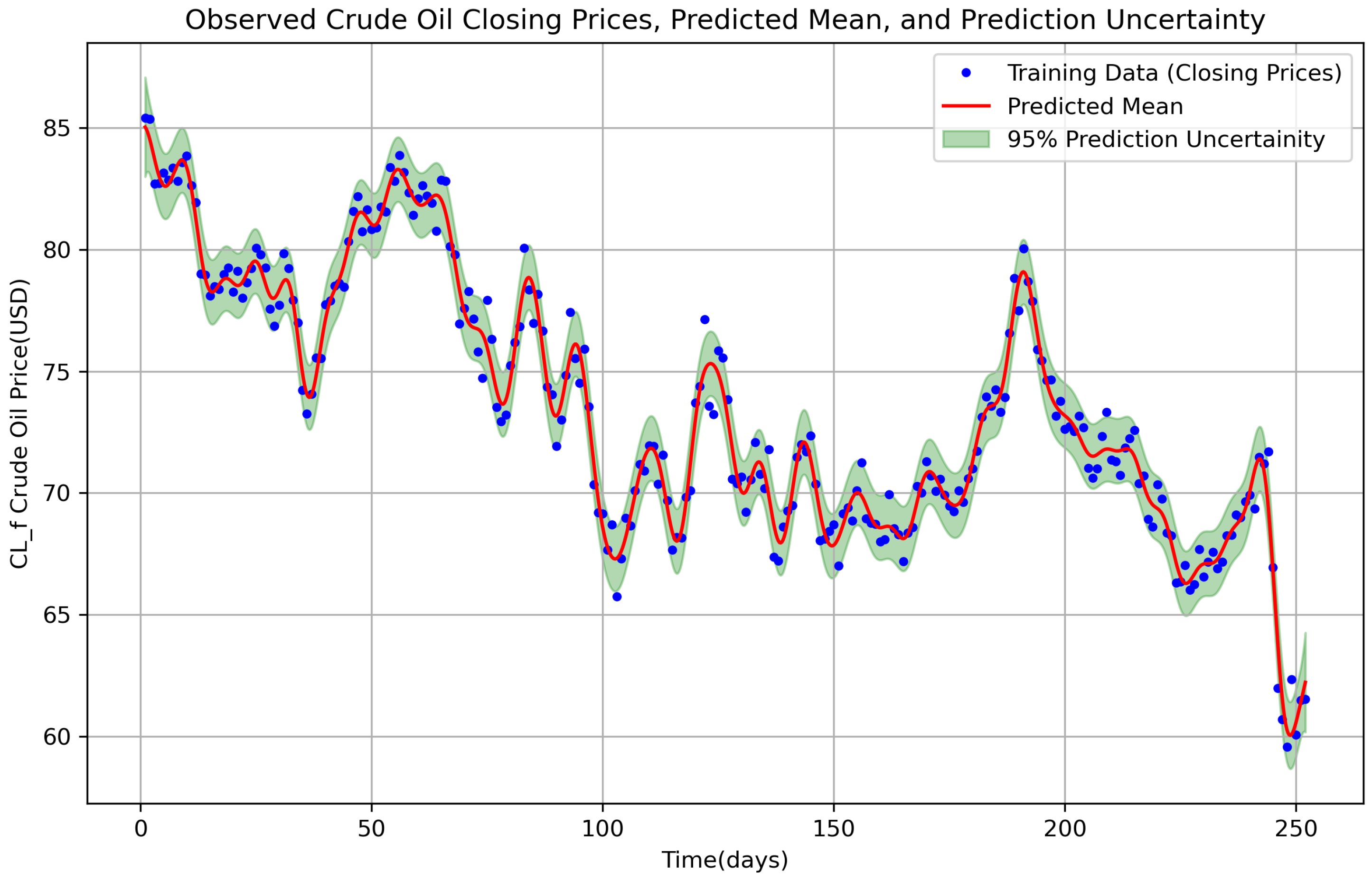
Once the optimal hyperparameters are obtained, we compute the predicted mean and the uncertainty region with (8) and (9). Figure 1 provides a visualization of the observed data, predicted mean, and uncertainty.

We compute the predicted mean for the closing price and the shaded uncertainty region and obtain Figure 1. More precisely, we obtain $N=1005$ interpolated closing commodity price data points, which is four times the original 252 closing commodity price data points. The predicted mean obtained by the non-parametric model GP regression follows the general pattern of the noise-free data (i.e., true data) at the dense data time point. This analysis agrees with [5].

3. Daily Change and Threshold Calculations

After obtaining the predicted closing price data for one year of crude oil in the augmented larger dataset, we compute the daily change and its percentage change. These values are added to the original dataframe. We then define a crash indicator using the standard deviation of the daily percentage change. Specifically, we set a threshold

$$KS=1.5\times \mathrm{standard}\mathrm{deviation}\left(\mathrm{daily}\mathrm{percentage}\mathrm{change}\right).$$

If the daily percentage change is less than $-KS$, we assign a value of 1 in the crash column; otherwise, we assign 0. This criterion helps us identify whether a significant drop in oil prices is likely in the upcoming days. In

Table 3. Predicted closing prices, daily change, daily percent change, and crash label, for $KS=0.3874$.

Index	Predicted Close	Daily Change	Daily Percent Change	Crash
0	85.0276	0.0000	0.0000	0
1	84.9473	−0.0803	−0.0944	0
2	84.8338	−0.1134	−0.1335	0
3	84.6918	−0.1420	−0.1674	0
4	84.5263	−0.1655	−0.1954	0
...	...	...	...	...
1000	61.3962	0.2089	0.3415	0
1001	61.6053	0.2091	0.3405	0
1002	61.8129	0.2077	0.3371	0
1003	62.0187	0.2057	0.3329	0
1004	62.2231	0.2044	0.3295	0

and 

Table 4. Original crude oil data, daily change, daily percent change, and crash labels, for $KS=2.9089$.

Index	Open	High	Low	Close	Volume	Daily Change	Daily Percent Change	Crash
0	85.9300	86.1100	84.0500	85.4100	343894	0.0000	0.0000	0
1	85.7000	86.1800	84.7500	85.3600	241343	−0.0500	−0.0585	0
2	85.3600	85.5100	82.5500	82.6900	259540	−2.6700	−3.1279	1
3	82.7900	83.4700	81.5600	82.7300	84468	0.0400	0.0484	0
4	82.6200	86.2800	81.8000	83.1400	76901	0.4100	0.4956	0
...	...	...	...	...	...	...	...	...
247	61.0300	61.7500	57.8800	59.5800	557655	−1.1200	−1.8451	0
248	58.3200	62.9300	55.1200	62.3500	592250	2.7700	4.6492	0
249	62.7100	63.3400	58.7600	60.0700	391826	−2.2800	−3.6568	1
250	60.2000	61.8700	59.4300	61.5000	306231	1.4300	2.3806	0
251	61.7000	62.6800	60.5900	61.5300	238068	0.0300	0.0488	0

, the Crash column is shown using a threshold value of $KS=0.3874$ and $2.9089$, respectively.

We consider a 1-year crude oil dataset as described in Section 2. We create a dataframe with 10 features for the predicted close price of crude oil data, and a similar procedure is applied to the original crude oil data as follows: Denote the daily change prices as $p_1,p_2,p_3,\dots ,p_{1004},p_{1005}$. Then, the new dataframe created will have 986 rows, where each row (consisting of 10 “features”) looks like the following:

$$\begin{array}{cc}& \mathrm{First}\mathrm{row}:p_1,p_2,\dots ,p_{10}\hfill \\ & \mathrm{Second}\mathrm{row}:p_2,p_3,\dots ,p_{11}\hfill \\ & \mathrm{Third}\mathrm{row}:p_3,p_4,\dots ,p_{12}\hfill \\ & ⋮\hfill \\ & \mathrm{Last}\mathrm{row}:p_{986},p_{987},\dots ,p_{995}.\hfill \end{array}$$

Once we create the dataframe, then we create a “target” variable Theta ($\theta$) that takes a value—either 1 or 0. This target variable will depend on the values of the next 10 days. Those are used to label each sample observation (i.e., each feature row as designed in the above) based on the daily change percent calculation. For instance, for the first row (i.e., $p_1,p_2,\dots ,p_{10}$), the target variable will be determined by whether it has a crash or not (as detailed below) on $p_{10},p_{11},\dots ,p_{19}$, etc.

Corresponding to the daily change prices $p_1,p_2,p_3,\dots ,p_{1004},p_{1005}$, we calculate the crash based on the daily percent change. To assign values to the target column of the dataframe, we count the number of crash values that are equal to 1 for the next 10 days. For example, to determine the target label for the row $p_1,\dots ,p_{10}$, we first count the crash values = 1, for the next 10 days, $p_{11},\dots ,p_{20}$. If this crash count is strictly greater than one (i.e., the number of crash values=1 for the next 10 days is $\ge 2$), we assign a value of 1 to the target column for the first row. Otherwise, we assign 0. Similarly, for the row $p_2,\dots ,p_{11}$, we conduct the crash count of the next 10 days, $p_{12},\dots ,p_{21}$, and if the crash count (for crash = 1) is greater than 1, we set the target value to 1; otherwise, we set it to 0. We apply the same procedure for the rest of the rows, labeling the target column with 1s and 0s for each row of the dataframe accordingly.

Finally, we apply machine learning algorithms where our sample observations comprise the daily change prices. For the analysis, we run the various classification algorithms. We provide the classification report and confusion matrix results in the next section.

4. Data Analysis Results

4.1. Data Analysis Procedures

We implement various supervised learning algorithms for dataset classification. To run supervised learning algorithms, we use the dataframes in

Table 5. Crude oil dataframe daily change for predicted closing price for augmented synthetic dataset.

Index	Daily Change 1	Daily Change 2	Daily Change 3	Daily Change 4	Daily Change 5	Daily Change 6	Daily Change 7	Daily Change 8	Daily Change 9	Daily Change 10	Target
0	0.000000	−0.080275	−0.113435	−0.142010	−0.165518	−0.183608	−0.196062	−0.202804	−0.203898	−0.199547	0
1	−0.080275	−0.113435	−0.142010	−0.165518	−0.183608	−0.196062	−0.202804	−0.203898	−0.199547	−0.190081	0
2	−0.113435	−0.142010	−0.165518	−0.183608	−0.196062	−0.202804	−0.203898	−0.199547	−0.190081	−0.175953	0
3	−0.142010	−0.165518	−0.183608	−0.196062	−0.202804	−0.203898	−0.199547	−0.190081	−0.175953	−0.157719	0
4	−0.165518	−0.183608	−0.196062	−0.202804	−0.203898	−0.199547	−0.190081	−0.175953	−0.157719	−0.136027	0
...	...	...	...	...	...	...	...	...	...	...	...
981	−0.659798	−0.614577	−0.559984	−0.497851	−0.430186	−0.359083	−0.286640	−0.214869	−0.145620	−0.080514	0
982	−0.614577	−0.559984	−0.497851	−0.430186	−0.359083	−0.286640	−0.214869	−0.145620	−0.080514	−0.020892	0
983	−0.559984	−0.497851	−0.430186	−0.359083	−0.286640	−0.214869	−0.145620	−0.080514	−0.020892	0.032228	0
984	−0.497851	−0.430186	−0.359083	−0.286640	−0.214869	−0.145620	−0.080514	−0.020892	0.032228	0.078170	0
985	−0.430186	−0.359083	−0.286640	−0.214869	−0.145620	−0.080514	−0.020892	0.032228	0.078170	0.116601	0

(augmented dataset with synthetic data) and

Table 6. Crude oil dataframe daily change for original data (i.e., no data augmentation).

Index	Daily Change 1	Daily Change 2	Daily Change 3	Daily Change 4	Daily Change 5	Daily Change 6	Daily Change 7	Daily Change 8	Daily Change 9	Daily Change 10	Target
0	0.000000	−0.050003	−2.669998	0.040001	0.409996	−0.290001	0.510002	−0.550003	0.760002	0.279999	0
1	−0.050003	−2.669998	0.040001	0.409996	−0.290001	0.510002	−0.550003	0.760002	0.279999	−1.220001	0
2	−2.669998	0.040001	0.409996	−0.290001	0.510002	−0.550003	0.760002	0.279999	−1.220001	−0.699997	0
3	0.040001	0.409996	−0.290001	0.510002	−0.550003	0.760002	0.279999	−1.220001	−0.699997	−2.930000	0
4	0.409996	−0.290001	0.510002	−0.550003	0.760002	0.279999	−1.220001	−0.699997	−2.930000	−0.050003	0
...	...	...	...	...	...	...	...	...	...	...	...
228	1.430000	−1.129997	0.629997	0.400002	−0.680000	0.260002	1.099998	0.019997	0.830002	−0.110001	1
229	−1.129997	0.629997	0.400002	−0.680000	0.260002	1.099998	0.019997	0.830002	−0.110001	0.650002	1
230	0.629997	0.400002	−0.680000	0.260002	1.099998	0.019997	0.830002	−0.110001	0.650002	0.269997	1
231	0.400002	−0.680000	0.260002	1.099998	0.019997	0.830002	−0.110001	0.650002	0.269997	−0.559998	1
232	−0.680000	0.260002	1.099998	0.019997	0.830002	−0.110001	0.650002	0.269997	−0.559998	2.120003	1

(original data), where we divide the dataset using the 60%–20%–20% split for training, validation, and testing, respectively. The data consists of 986 samples (or, rows, as described in Section 3) from 1-year data for crude oil. In the training dataset, there is a data imbalance with the class labels. There are 503 samples classified as label 0, while the remaining 88 samples are classified as label 1. To address the data imbalance, we implement an oversampling technique on the training dataset. This means increasing the number of instances in the minority class (i.e., class 1) to match the number of instances in the majority class (i.e., class 0). Essentially, oversampling works by repeatedly sampling from the minority class to increase its size, ensuring that it balances with the majority class in the dataset.

Then, we run the various algorithms like Logistic Regression (LR), K Nearest Neighbors (KNN), Random Forest (RF), Support Vector Machine (SVM), Decision Tree (DT), Deep Learning (DL), LSTM, and the LSTM Method with Batch Normalizer (BN), and the table results of the performance metrics follow in Section 4.2.

4.2. Performance Metrics of Machine Learning Models

4.2.1. Confusion Matrix and Performance Metrics

The following quantities are well-known:

• True Positive (TP): The number of positive instances correctly predicted as positive.
• True Negative (TN): The number of negative instances correctly predicted as negative.
• False Positive (FP): The number of negative instances incorrectly predicted as positive.
• False Negative (FN): The number of positive instances incorrectly predicted as negative.

For a binary classification problem with two class labels, positive (P) and negative (N), the confusion matrix is organized as follows:

$$\begin{array}{ccc}\mathrm{Actual}\setminus \mathrm{Predicted}& P& N\\ P& TP& FN\\ N& FP& TN\end{array}$$

Before performing any analysis, it is important to define evaluation metrics to assess the quality of predictions. They provide different perspectives on the model’s performance:

• Recall (Sensitivity or True Positive Rate): This measures how well the model identifies actual positive instances. It is defined as

  $$\mathrm{Recall}={\displaystyle \frac{TP}{TP+FN}}.$$
• Precision (Positive Predictive Value): This measures how accurate the positive predictions are. It is defined as

  $$\mathrm{Precision}={\displaystyle \frac{TP}{TP+FP}}.$$
• Accuracy: This measures the overall correctness of the model. It is defined as

  $$\mathrm{Accuracy}={\displaystyle \frac{TP+TN}{TP+FP+TN+FN}}.$$

Defining these metrics upfront is crucial for our machine learning analysis, enabling us to understand and select the most suitable models when working with both the original and synthetic data. In our analysis, we use classes 1 (big fluctuation in commodity) and 0 (regular fluctuation in commodity), as described earlier.

4.2.2. Crude Oil (CL=F) Data for One Year (from 15 April 2024 to 15 April 2025)

After applying oversampling to address the data imbalance (503 samples for label 0 and 88 for label 1), the machine learning models show improved performance on the minority class when we compare them with the original data. We provide the results in

Table 7. Performance metrics for traditional machine learning models for CL=F 1-year predicted data.

Models	$\mathit{\theta }$	Precision	Recall	F1-Score	Support	Accuracy
LR	0	1.00	0.94	0.97	172	0.94
	1	0.70	1.00	0.83	26
KNN	0	0.97	0.92	0.95	172	0.91
	1	0.62	0.81	0.70	26
RF	0	0.97	0.97	0.97	172	0.94
	1	0.78	0.81	0.81	26
SVM	0	1.00	0.96	0.98	172	0.96
	1	0.79	1.00	0.88	26
DT	0	0.96	0.94	0.95	172	0.92
	1	0.67	0.77	0.71	26

,

Table 8. Performance metrics for neural networks for CL=F 1-year predicted data.

Models	$\mathit{\theta }$	Precision	Recall	F1-Score	Support	Accuracy
DL	0	0.99	0.95	0.97	172	0.95
	1	0.74	0.96	0.83	26
LSTM	0	1.00	0.95	0.97	172	0.95
	1	0.74	1.00	0.85	26
BN	0	1.00	0.94	0.97	172	0.94
	1	0.70	1.00	0.83	26

,

Table 9. Performance metrics for traditional machine learning models for CL=F 1-year original data.

Models	$\mathit{\theta }$	Precision	Recall	F1-Score	Support	Accuracy
LR	0	0.78	0.64	0.70	39	0.55
	1	0.07	0.12	0.09	8
KNN	0	0.75	0.46	0.57	39	0.43
	1	0.09	0.25	0.13	8
RF	0	0.82	0.95	0.88	39	0.79
	1	0.00	0.00	0.00	77
SVM	0	0.83	1.00	0.91	39	0.83
	1	0.00	0.00	0.00	8
DT	0	0.76	0.64	0.69	39	0.53
	1	0.00	0.00	0.00	8

and

Table 10. Performance metrics for neural networks for CL=F 1-year original data.

Models	$\mathit{\theta }$	Precision	Recall	F1-Score	Support	Accuracy
DL	0	0.78	0.72	0.75	39	0.60
	1	0.00	0.00	0.00	8
LSTM	0	0.80	0.62	0.70	39	0.55
	1	0.12	0.25	0.16	8
BN	0	0.89	0.82	0.85	39	0.77
	1	0.36	0.50	0.42	8

. The results in Table 7 and Table 8 are for the augmented dataset.

For the original dataset (with no augmentation with synthetic data), there are 119 samples labeled as class 0 and 20 as class 1. After applying the oversampling technique, the results are provided in Table 9 and Table 10.

Oversampling also improves the neural networks’ performance on the minority class (label 1). The results displayed in Table 7 and Table 8 are better than the results in Table 9 and Table 10.

From the above tables, we observe the superiority in performance of both traditional machine learning (ML) and neural network (NN) models for the 1-year predicted data over the 1-year original data. This can be attributed to two major factors. First, the GP regression process smooths out the inherent noise and volatility present in commodity time series such as our crude oil price data. This smoothing reduces irregular fluctuations and high-frequency components, which allows models to learn more coherent and separable decision boundaries. Second, the predicted dataset shows lower variability in model performance because all models are trained on a more regular and noise-filtered version of the underlying dynamics. On the other hand, the original dataset contains abrupt jumps and microstructure noise, which can negatively affect learning and may cause overfitting or underfitting depending on the model.

As a result, there is a greater spread in model accuracy for the original data, reflecting differences in how each model responds to noise. For example, in the original dataset, accuracy ranges from 0.43 for KNN and 0.53 for the Decision Tree, both of which are sensitive to local noise, to 0.79 for Random Forest and 0.83 for SVM, which are more robust and able to capture complex patterns (i.e., nonlinear relationships). In contrast, the predicted dataset results in much more consistent performance, with accuracy variation limited to only 0.05 for ML models and 0.01 for NN models. This is because smoother and less noisy data allow all models, including simpler ones, to perform effectively.

4.2.3. Crude Oil (CL=F) Data for 10 Years (from 15 April 2015 to 15 April 2025)

We now apply machine learning techniques to 10 years of CL=F data. The original dataset, augmented with quarterly intervals, while maintaining the original starting and ending time points, will be shown to improve prediction accuracy.

The data-dependent initialization improved the log marginal likelihood from $-113541.1936$ to $-888.0075$, reflecting a better model fit. This is described in

Table 11. Optimal hyperparameter values from 15 April 2015 to 15 April 2025.

Hyperparameter	Initialization	Normalized Optimal Values	Denormalized Optimal Values
Noise Variance (${\sigma }_n^2$)	0.001012	0.017585	5.718099
Signal Variance (${\sigma }_f^2$)	0.004048	1.100225	357.762116
Length Scale (ℓ)	0.001377	0.010260	7.448797

. The tuned length scale of $7.448797$ suggests oil price correlations decay over about 7 trading days.

Table 12. Predicted closing prices, daily change, percentage change, and crash label for 10 yr.

Index	Predicted Close	Daily Change	Daily Change Percent	Crash
0	56.553343	0.000000	0.000000	0
1	56.468885	−0.084458	−0.149342	0
2	56.391173	−0.077712	−0.137619	0
3	56.320490	−0.070683	−0.125344	0
4	56.257094	−0.063396	−0.112563	0
...	...	...	...	...
10,052	60.494617	0.097117	0.160796	0
10,053	60.626566	0.131949	0.218117	0
10,054	60.792239	0.165673	0.273267	0
10,055	60.990280	0.198041	0.325767	0
10,056	61.219103	0.228823	0.375180	0

presents the predicted closing prices and other features for 10 years.

Table 13. Predicted crude oil daily percentage change features (window size = 10) and target labels for crash detection.

Index	Daily Change 1	Daily Change 2	Daily Change 3	Daily Change 4	Daily Change 5	Daily Change 6	Daily Change 7	Daily Change 8	Daily Change 9	Daily Change 10	Target
0	0.000000	−0.084458	−0.077712	−0.070683	−0.063396	−0.055880	−0.048163	−0.040279	−0.032258	−0.024136	0
1	−0.084458	−0.077712	−0.070683	−0.063396	−0.055880	−0.048163	−0.040279	−0.032258	−0.024136	−0.015946	0
2	−0.077712	−0.070683	−0.063396	−0.055880	−0.048163	−0.040279	−0.032258	−0.024136	−0.015946	−0.007726	0
3	−0.070683	−0.063396	−0.055880	−0.048163	−0.040279	−0.032258	−0.024136	−0.015946	−0.007726	0.000490	0
4	−0.063396	−0.055880	−0.048163	−0.040279	−0.032258	−0.024136	−0.015946	−0.007726	0.000490	0.008665	0
...	...	...	...	...	...	...	...	...	...	...	...
10,033	−0.421399	−0.413875	−0.403301	−0.389730	−0.373247	−0.353962	−0.332011	−0.307557	−0.280786	−0.251903	0
10,034	−0.413875	−0.403301	−0.389730	−0.373247	−0.353962	−0.332011	−0.307557	−0.280786	−0.251903	−0.221135	0
10,035	−0.403301	−0.389730	−0.373247	−0.353962	−0.332011	−0.307557	−0.280786	−0.251903	−0.221135	−0.188726	0
10,036	−0.389730	−0.373247	−0.353962	−0.332011	−0.307557	−0.280786	−0.251903	−0.221135	−0.188726	−0.154931	0
10,037	−0.373247	−0.353962	−0.332011	−0.307557	−0.280786	−0.251903	−0.221135	−0.188726	−0.154931	−0.120019	0

provides the results for the predicted daily percentage change of crude oil (window size = 10) and the target labels for crash detection. On the other hand,

Table 14. Original crude oil price data (without synthetic date), daily change, percentage change, and crash labels.

Index	Open	High	Low	Close	Volume	Daily Change	Daily Change Percent	Crash
0	53.549999	56.689999	53.389999	56.389999	508904	0.000000	0.000000	0
1	55.919998	57.419998	55.070000	56.709999	413134	0.320000	0.567476	0
2	56.560001	56.880001	55.310001	55.740002	230623	−0.969997	−1.710452	0
3	56.160000	57.169998	54.849998	56.380001	112382	0.639999	1.148187	0
4	56.410000	56.910000	55.009998	55.259998	354244	−1.120003	−1.986525	0
...	...	...	...	...	...	...	...	...
2510	61.029999	61.750000	57.880001	59.580002	557655	−1.119999	−1.845138	0
2511	58.320000	62.930000	55.119999	62.349998	592250	2.769997	4.649205	0
2512	62.709999	63.340000	58.759998	60.070000	391826	−2.279999	−3.656774	0
2513	60.200001	61.869999	59.430000	61.500000	306231	1.430000	2.380557	0
2514	61.700001	62.680000	60.590000	61.529999	238068	0.029999	0.048779	0

provides original crude oil price data (without synthetic date), daily change, percentage change, and crash labels, and

Table 15. Original crude oil daily percentage change features (window size = 10) and crash target labels.

Index	Daily Change 1	Daily Change 2	Daily Change 3	Daily Change 4	Daily Change 5	Daily Change 6	Daily Change 7	Daily Change 8	Daily Change 9	Daily Change 10	Target
0	0.000000	0.320000	−0.969997	0.639999	−1.120003	0.900002	1.580002	−0.590000	−0.160000	0.070000	0
1	0.320000	−0.969997	0.639999	−1.120003	0.900002	1.580002	−0.590000	−0.160000	0.070000	1.520000	0
2	−0.969997	0.639999	−1.120003	0.900002	1.580002	−0.590000	−0.160000	0.070000	1.520000	1.049999	0
3	0.639999	−1.120003	0.900002	1.580002	−0.590000	−0.160000	0.070000	1.520000	1.049999	−0.480000	0
4	−1.120003	0.900002	1.580002	−0.590000	−0.160000	0.070000	1.520000	1.049999	−0.480000	−0.220001	0
...	...	...	...	...	...	...	...	...	...	...	...
2491	1.430000	−1.129997	0.629997	0.400002	−0.680000	0.260002	1.099998	0.019997	0.830002	−0.110001	0
2492	−1.129997	0.629997	0.400002	−0.680000	0.260002	1.099998	0.019997	0.830002	−0.110001	0.650002	0
2493	0.629997	0.400002	−0.680000	0.260002	1.099998	0.019997	0.830002	−0.110001	0.650002	0.269997	0
2494	0.400002	−0.680000	0.260002	1.099998	0.019997	0.830002	−0.110001	0.650002	0.269997	−0.559998	0
2495	−0.680000	0.260002	1.099998	0.019997	0.830002	−0.110001	0.650002	0.269997	−0.559998	2.120003	0

shows the original crude oil daily percentage change features (window size = 10) and crash target labels.

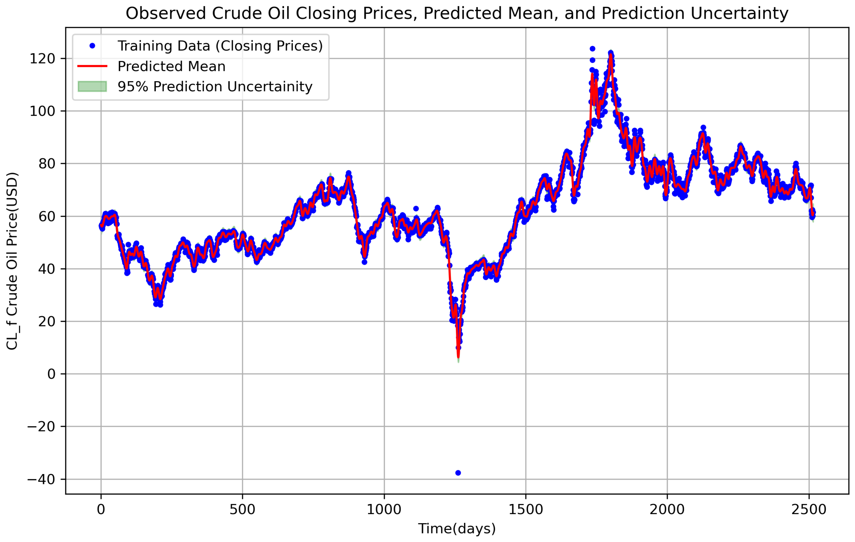
The column “Crash” in Table 12 and Table 14 is calculated with the threshold $KS=0.42714$ and $7.21208$ considered one standard deviation of the daily percent change. As a result, the dataframes in Table 13 and Table 15 expand to dimensions $10,038\times 11$ and $2496\times 11$, respectively (including the target variable column). Figure 2 demonstrates the predicted mean along with its uncertainty region. The results obtained during this 10-year period are also promising, as shown in

Table 16. Performance metrics for traditional machine learning models for CL=F 10-year predicted data (augmented synthetic dataset).

Models	$\mathit{\theta }$	Precision	Recall	F1-Score	Support	Accuracy
LR	0	1.00	0.90	0.94	1898	0.90
	1	0.35	0.93	0.50	110
KNN	0	0.99	0.95	0.97	1898	0.94
	1	0.48	0.76	0.59	110
RF	0	0.98	0.98	0.98	1898	0.96
	1	0.67	0.61	0.64	110
SVM	0	0.98	0.95	0.97	1898	0.94
	1	0.44	0.65	0.53	110
DT	0	0.98	0.94	0.96	1898	0.93
	1	0.43	0.75	0.55	110

and

Table 17. Performance metrics for neural networks for CL=F 10-year predicted data (augmented synthetic dataset).

Models	$\mathit{\theta }$	Precision	Recall	F1-Score	Support	Accuracy
DL	0	1.00	0.91	0.95	1898	0.91
	1	0.37	0.94	0.54	110
LSTM	0	1.00	0.92	0.96	1898	0.93
	1	0.42	0.95	0.58	110
BN	0	1.00	0.92	0.96	1898	0.92
	1	0.41	0.95	0.57	110

.

Finally, in the following analysis, we apply the aforementioned machine learning classifiers to the original CL=F 10-year commodity price data. By comparing the classifiers’ accuracy results, we clearly observe that the denoised data computed at dense time points yield the highest accuracy. The methods previously employed for the synthetic data at dense time points are similarly applied here. We construct the dataframe in Table 15, indicating 2496 samples, each with 10 features and one target, consistent with our synthetic data procedure. Upon calculating the threshold we obtain KS = 7.212088. Subsequently, we apply the machine learning classifiers to evaluate the performance improvements achieved using densely sampled data points. For this dataset, we have 119 training samples labeled as class 0 and 20 as class 1. The same oversampling techniques used for the densified data were applied here as well. The results are summarized in

Table 18. Performance metrics for traditional machine learning models on the original CL=F 10-year data (i.e., no augmented synthetic data).

Models	$\mathit{\theta }$	Precision	Recall	F1-Score	Support	Accuracy
LR	0	0.99	0.85	0.91	489	0.84
	1	0.06	0.45	0.11	11
KNN	0	0.98	0.99	0.98	489	0.97
	1	0.12	0.09	0.11	11
RF	0	0.98	1.00	0.99	489	0.98
	1	0.00	0.00	0.00	11
SVM	0	0.98	1.00	0.99	489	0.98
	1	0.00	0.00	0.00	11
DT	0	0.98	0.99	0.98	489	0.97
	1	0.00	0.00	0.00	11

and

Table 19. Performance metrics for neural networks for original CL=F 10-year data (i.e., no augmented synthetic data).

Models	$\mathit{\theta }$	Precision	Recall	F1-Score	Support	Accuracy
DL	0	0.98	0.98	0.98	489	0.91
	1	0.25	0.27	0.26	11
LSTM	0	0.99	0.99	0.99	489	0.97
	1	0.42	0.45	0.43	11
BN	0	0.99	0.96	0.97	489	0.94
	1	0.17	0.36	0.24	11

.

Many of the classifiers fail to detect any crash signals on the original data with fewer points (giving zero precision, recall, and F1-scores) for $\theta =1$, as we can see in Table 18 and Table 19. We compare the classifiers obtained from the densed time points in Table 16 and Table 17. It is worth noting that for 10-year data, there are already a good number of data points, and thus the synthetic set of data marginally improves the prediction results. However, as we have seen before, the improvement is much better for 1-year data. The number of data points in 1-year data is small, and hence the incorporation of synthetic data makes more improvement to the original results.

Even for the 10-year data, despite the similar accuracies of the machine learning (ML) and neural network (NN) models on both the 10-year original and predicted data, the ML and NN models trained on the original data struggle to detect class 1, as evidenced by the low precision, recall, and F1-scores for $\theta =1$. In contrast, the predicted data yields better performance for class 1 detection, even with a limited dataset such as the 1-year data. This suggests that GPR is particularly effective for tasks like ML and NN when working with smaller datasets, as supported by [3]. However, using a larger dataset, such as 10 years of data, still outperforms the ML and NN results on the predicted data when compared to the original data, particularly in terms of precision, recall, and F1-score for $\theta$.

The above results provide the analysis for CL=F data for various time frames. It is very clear from the tables that for shorter time intervals, the synthetic data generation provides much more improvement to the prediction. The synthetic data provides an additional source of data that augments the original dataset. As observed above, for a shorter time frame, where there is a lack of sufficient data points in the original set, the presented method helps to boost the analysis and provide a much better prediction.

5. Conclusions

In this paper, we introduce Gaussian process (GP) regression as a method to denoise observed financial data and generate predictions at densely interpolated time points. Specifically, we apply our methodology to one-year and ten-year datasets of CL=F crude oil prices. Using a Gaussian kernel with data-dependent initialization to optimize hyperparameters, we compute predictive means and uncertainty regions (i.e., confidence interval).

Subsequently, we construct a dataset that incorporates ten predictive features derived from the mean predictions, alongside the calculated daily changes and their percentages. We utilize the standard deviation of the daily change percent, multiplying it by a scalar as much as we need the threshold to be, to decide whether the daily change percent is categorized as under crash or not; then, later, we apply the crash count technique over subsequent 10-day intervals as class labels, enabling the application of various machine learning algorithms. Our analysis reveals that the predictive means obtained via GP regression yield higher accuracy compared to the original sparse data within an identical time period. Thus, data densification using GP regression enhances the detection of potential market crashes or fluctuations over the subsequent 10-day period.

As shown in this paper, the improvement in prediction is significantly greater for one year’s worth of data (compared to a bigger dataset). Since there are only a few data points in a one-year dataset, adding synthetic data improves the initial findings even more. This suggests that the proposed method can be implemented for small-data analysis. There are many occasions when procuring a large dataset is difficult. In those cases, the generation of synthetic data and the corresponding analysis presented in this paper can be implemented. The predictions are of importance for practitioners and policymakers.

References

- Tolstoy, A. Matched Field Processing for Underwater Acoustics; World Scientific: Singapore, 1993. [Google Scholar]
- Caviedes-Nozal, D.; Riis, N.A.; Heuchel, F.M.; Brunskog, J.; Gerstoft, P.; Fernandez-Grande, E. Gaussian processes for sound field reconstruction. J. Acoust. Soc. Am. 2021, 149, 1107–1119. [Google Scholar] [CrossRef]
- Frederick, C.; Michalopoulou, Z. Seabed classification and source localization with Gaussian processes and machine learning. JASA Express Lett. 2022, 2, 084801. [Google Scholar] [CrossRef] [PubMed]
- Michalopoulou, Z.-H.; Gerstoft, P. Inversion in an uncertain ocean using Gaussian processes. J. Acoust. Soc. Am. 2023, 153, 1600–1611. [Google Scholar] [CrossRef] [PubMed]
- Michalopoulou, Z.-H.; Gerstoft, P.; Caviedes-Nozal, D. Matched field source localization with Gaussian processes. JASA Express Lett. 2021, 1, 064801. [Google Scholar] [CrossRef] [PubMed]
- Murphy, K.P. Machine Learning: A Probabilistic Perspective; MIT Press: Cambridge, MA, USA, 2012. [Google Scholar]
- Rasmussen, C.E.; Williams, C.K. Gaussian Processes for Machine Learning; MIT Press: Cambridge, MA, USA, 2006. [Google Scholar]
- Valentine, A.P.; Sambridge, M. Gaussian process models—I. A framework for probabilistic continuous inverse theory. Geophys. J. Int. 2020, 220, 1632–1647. [Google Scholar] [CrossRef]
- Valentine, A.P.; Sambridge, M. Gaussian process models—II. Lessons for discrete inversion. Geophys. J. Int. 2020, 220, 1648–1656. [Google Scholar] [CrossRef]
- SenGupta, I.; Nganje, W.; Hanson, E. Refinements of Barndorff-Nielsen and Shephard model: An analysis of crude oil price with machine learning. Ann. Data Sci. 2021, 8, 39–55. [Google Scholar] [CrossRef]
- Hui, X.; Sun, B.; Jiang, H.; SenGupta, I. Analysis of stock index with a generalized BN-S model: An approach based on machine learning and fuzzy parameters. Stoch. Anal. Appl. 2023, 41, 938–957. [Google Scholar] [CrossRef]
- Lin, M.; SenGupta, I.; Wilson, W. Estimation of VaR with jump process: Application in corn and soybean markets. Appl. Stoch. Model. Bus. Ind. 2024, 40, 1337–1354. [Google Scholar] [CrossRef]
- Awasthi, S.; SenGupta, I.; Wilson, W.; Lakkakula, P. Machine learning and neural network based model predictions of soybean export shares from US Gulf to China. Stat. Anal. Data Mining Asa Data Sci. J. 2022, 15, 707–721. [Google Scholar] [CrossRef]
- Shoshi, H.; SenGupta, I. Hedging and machine learning driven crude oil data analysis using a refined Barndorff-Nielsen and Shephard model. Int. J. Financ. Eng. 2021, 8, 2150015. [Google Scholar] [CrossRef]
- Shoshi, H.; Hanson, E.; Nganje, W.; SenGupta, I. Stochastic analysis and neural network-based yield prediction with precision agriculture. J. Risk Financ. Manag. 2021, 14, 397. [Google Scholar] [CrossRef]
- Roberts, M.; SenGupta, I. Infinitesimal generators for two-dimensional Lévy process-driven hypothesis testing. Ann. Financ. 2020, 16, 121–139. [Google Scholar] [CrossRef]
- Roberts, M.; SenGupta, I. Sequential Hypothesis Testing in Machine Learning, and Crude Oil Price Jump Size Detection. Appl. Math. Financ. 2020, 27, 374–395. [Google Scholar] [CrossRef]
- Bisht, A.; Chahar, A.; Kabthiyal, A.; Goel, A. Stock prediction using Gaussian process regression. In Proceedings of the 2022 6th International Conference on Computing Methodologies and Communication (ICCMC), Erode, India, 29–31 March 2022; IEEE: New York, NY, USA, 2022; pp. 693–699. [Google Scholar]
- Chen, Z. Gaussian Process Regression Methods and Extensions for Stock Market Prediction. Ph.D. Dissertation, University of Leicester, Leicester, UK, 2017. [Google Scholar]
- Gebreslasie, M.; SenGupta, I. Synthetic stocks and market movement estimation: An analysis with Gaussian process, drawdown, and data science. 2025; submitted. [Google Scholar]
- Ulapane, N.; Thiyagarajan, K.; Kodagoda, D. Hyper-parameter initialization for squared exponential kernel-based gaussian process regression. In Proceedings of the 2020 15th IEEE Conference on Industrial Electronics and Applications (ICIEA), Kristiansand, Norway, 21–25 June 2020; IEEE: New York, NY, USA, 2020; pp. 1154–1159. [Google Scholar]
Figure 1.
Crude oil data trend (15 April 2024 to 15 April 2025) for the noisy data (blue dots) for one year and the predicted mean for the closing price at quarterly time steps obtained using GP regression (solid red line). The shaded area is the uncertainty of the mean prediction obtained via the square root of the diagonal elements of , given by .
Figure 2.
CL=F oil price data trend (15 April 2015 to 15 April 2025) for the noisy data (blue dots) for two years and the predicted mean at densed points (virtual time steps) obtained for (i.e., denormalized) using GP regression (solid red line). The shaded area is the uncertainty of the mean prediction obtained via the square root of the diagonal elements of , given by .