Performance of Commodity Futures-Based Dynamic Portfolios ^†

Abstract

This paper analyzes the return performance of various commodity futures-based dynamic portfolios over the period from 31 January 1986 to 31 July 2023. By constructing 30 distinct portfolios categorized by style and performance, we assess their potential for enhancing the performance of traditional portfolios consisting of equity and bonds. We find that most commodity portfolios do not offer statistically significant returns, either in terms of average or risk-adjusted returns. Only the portfolios in the basis category and portfolios in the term structure category exhibit significantly positive risk-adjusted returns, indicating their potential value for portfolio enhancement. The performance of these portfolios is not different in pre-financialization and financialization periods.

1. Introduction

Over the years, investors have regarded commodities as a distinct asset class that offers high returns, provides diversification benefits, and protects against inflation. Several studies have provided evidence supporting higher returns for tactical portfolios of commodity futures, including those by [1,2,3,4,5,6,7,8]. In their influential paper, Gorton and Rouwenhorst analyzed a basket of 36 commodity futures from 1959 to 2004. They found that this basket offered returns and risk premiums comparable to equities, was negatively correlated with equity and bond returns, and served as a hedge against both expected and unexpected inflation. Building on these findings, ref. [3] reinforced the conclusions of Gorton and Rouwenhorst but also pointed out that “[historically] the average annualized excess return of the average individual commodity future has been approximately zero, and commodity futures returns have been largely uncorrelated with one another. However, the annualized excess return of a rebalanced portfolio of commodity futures can be ‘equity-like’”.

Refs. [4,7] provide strong evidence of significant positive returns across various ranking and holding periods, extending up to 12 months, through momentum strategies. Notably, ref. [7] report returns of 0.7% for low-return momentum portfolios and 13.1% for high-return momentum portfolios. Ref. [4] identify 13 profitable momentum strategies in the commodity futures markets, yielding an average annual return of 9.38% by strategically reallocating wealth toward top-performing commodities and away from the underperformers. Additionally, refs. [4,8] introduce innovative tactical strategies that incorporate term structure information, alongside momentum strategies in some cases, to achieve substantial returns. [4] report annualized alphas of 10.14% and 12.66% for momentum and term structure strategies, respectively. However, a combined double-sort strategy that leverages both components generates an impressive return of approximately 21.02%.

In this paper, we examine the return performance of six buy-and-hold and twenty-four tactical portfolios of commodity futures. Traditionally, only those directly or indirectly involved in commodity production or consumption participated in the commodity futures market to mitigate the risk of price changes; however, over the past two and a half decades, changes in the commodity futures market have provided a low-cost vehicle for investors to include commodities in well-diversified portfolios. Institutional investors and large traders, with no interest in the workings of the underlying markets, began to participate in the commodity futures markets. Consequently, there was a significant influx of capital from institutional investors and large traders. This increased participation in both equity and commodity futures markets may have an integrating effect, reducing segmentation, equating risk prices, and increasing the exposure of futures markets to other financial markets; therefore, it is pertinent to ask whether financialization has impacted the benefits of investing in commodity futures markets.

To assess performance, we analyze both the monthly average returns and the risk-adjusted returns of six traditional buy-and-hold portfolios alongside twenty-four tactical portfolios from January 1986 to July 2023. We employ a dataset of 29 commodity futures to construct five sector-specific buy-and-hold portfolios, including foods and fibers, grains and oilseeds, livestock, energy, and precious metals, as well as an equally weighted portfolio that covers all these sectors. These portfolios serve as benchmarks against which we compare the efficacy of various investment strategies.

In exploring the strategic opportunities available within commodity futures, we harness data on the basis and excess speculation. Building on previous empirical research that associates the basis and excess speculation of commodity futures with their return characteristics, we seek to exploit this information by creating portfolios based on these criteria. According to [2], portfolios that select commodity futures based on prior returns and the futures basis, particularly with lower-than-average inventories, are poised to achieve superior risk premiums, aligning with the theory of storage predictions; thus, these basis portfolios integrate a unique risk element unrelated to inventory fluctuations, which is recognized with higher average returns.

Furthermore, portfolios based on excess speculation are designed following the notion that commodity producers and consumers offload price volatility risks to speculators, as discussed by [9,10]. When short hedgers outnumber long hedgers, the current futures price tends to underestimate the future maturity price, known as normal backwardation. Conversely, if hedgers predominantly hold long positions, the current price will likely exceed the future maturity price to motivate speculators to adopt short positions, a situation referred to as contango. Given that commodity returns are influenced by hedger demand, excess speculation could provide a valuable tactical approach. As further supported by [11,12], hedging pressure—which reflects genuine hedging demands—is a plausible proxy for broader nonmarketable risks.

Additionally, we developed nine portfolios, each based on return momentum and term structure. [4] describe how momentum strategies, which capitalize on markets’ tendencies toward backwardation or contango, are not just compensations for risk but also offer low correlation with traditional asset classes, making them excellent for portfolio diversification. Our review extends this analysis to recent market conditions to validate the efficacy of momentum strategies as diversifiers. Similarly, term structure portfolios, which capitalize on differences in risk–return characteristics across various contract maturities, offer insights into reducing volatility and enhancing returns through strategic contract selection.

The main result of the paper is that most portfolios do not offer statistically significant returns in terms of both average and risk-adjusted returns, similar to the finding of [13]. Only the Highb portfolio in the Basis category and the HighTS12 portfolio in the term structure category exhibit significantly positive risk-adjusted returns, indicating their potential value for enhancing a portfolio. Conversely, many portfolios show negative or non-significant returns, underscoring their limited importance for inclusion in a traditional portfolio to improve performance.

The major contribution of the paper is the assessment of 30 distinct portfolios, categorized by style and performance, to evaluate their potential for enhancing traditional equity and bond portfolios. The study examines raw returns without incorporating risk-free rates and employs time series regression in a factor model format. We conclude that long-only portfolios typically do not yield statistically significant average returns, but combining long and short positions might be an effective strategy.

The remainder of this paper is organized as follows: Section 2 outlines the dataset used and details formation on the commodity futures return series. Section 3 delves into the development of the various buy-and-hold and tactical commodity futures portfolios and analyzes their respective returns. In Section 4, we present the methodology and empirical results of portfolio performance analysis. Finally, Section 5 provides concluding observations.

2. Data and Commodity Futures Return Construction

The futures prices of the 29 commodity futures used in this study were obtained from Barchart.com Inc. We extracted the price series information from 1 January 1986 to 31 July 2023. The breakdown of the commodities by sector is as follows: six from foods and fibers, nine from grains and oilseeds, four from livestock, five from energy, and five from precious metals. All commodities and the time period considered for each commodity are provided in

Table 1. Commodity futures contracts and period covered.

Food and Fibers	Exchange	Period Covered
Cocoa (CC)	ICE	1/01/1986 to 7/31/2023
Coffee (KC)	ICE	1/01/1986 to 7/31/2023
Orange Juice (JO)	ICE	1/01/1986 to 7/31/2023
Sugar #11 (SB)	ICE	1/01/1986 to 7/31/2023
Cotton (CT)	ICE	1/01/1986 to 7/31/2023
Lumber (LB)	CME	1/01/1986 to 7/31/2023
Grains and Oilseeds
Corn #2 (C_)	CBOT	1/01/1986 to 7/31/2023
Oats (O_)	CBOT	1/01/1986 to 7/31/2023
Rough Rice #2 (RR)	CBOT	8/20/1986 to 7/31/2023
Soybeans (S_)	CBOT	1/01/1986 to 7/31/2023
Soybean Meal (SM)	CBOT	1/01/1986 to 7/31/2023
Soybean Oil (BO)	CBOT	1/01/1986 to 7/31/2023
Wheat (W_)	CBOT	1/01/1986 to 7/31/2023
Barley (WA)/NCDEX Barley	WCE/ NCDEX	5/24/1989 to 12/13/2006 and 12/14/2006 to 7/31/2023
Canola (WC)	WCE	1/01/1986 to 7/31/2023
Livestock
Feeder Cattle (FC)	CME	1/01/1986 to 7/31/2023
Live Cattle (LC)	CME	1/01/1986 to 7/31/2023
Lean Hogs (LH)	CME	1/01/1986 to 7/31/2023
Pork Bellies (PB)	CME	1/01/1986 to 12/31/2009
Energy
Crude Oil (CL)	NYMEX	1/01/1986 to 7/31/2023
Heating Oil #2 (HO)	NYMEX	1/01/1986 to 7/31/2023
Unleaded Gas (HU/RB)	NYMEX	1/01/1986 to 7/31/2023
Natural Gas (NG)	NYMEX	4/4/1990 to 7/31/2023
Propane (PN)	NYMEX	8/24/1987 to 8/31/2009
Precious Metals
Copper (HG)	NYMEX	1/01/1986 to 7/31/2023
Gold (GC)	NYMEX	1/01/1986 to 7/31/2023
Palladium (PA)	NYMEX	1/01/1986 to 7/31/2023
Platinum (PL)	NYMEX	1/01/1986 to 7/31/2023
Silver (SI)	NYMEX	1/01/1986 to 7/31/2023

Note: Table 1 shows the different commodities and the periods covered in this study. The second column shows the name of the exchange where the commodity is traded. The ticker symbol for each commodity is given within the parentheses next to the commodity.

.

In order to construct the futures return series, we follow the procedure outlined by [4] whereby, for each particular commodity, we roll the daily futures prices of the nearby contract over to the next next-nearby contract one month prior to the maturity of the nearby contract. This procedure is performed for the entire dataset of commodity futures to generate a continuous series of futures prices. We denote the daily price of futures expiring in the T period by $\left({\mathrm{F}}_{\mathrm{d},\mathrm{T}}\right)$. We compute the daily return series $\left({\mathrm{r}}_{\mathrm{d}}\right)$, for each commodity future by taking the natural logarithm difference of the daily futures prices on two consecutive trading days (${\mathrm{r}}_{\mathrm{d}}=\mathrm{L}\mathrm{o}\mathrm{g}\left({\mathrm{F}}_{\mathrm{d},\mathrm{T}}\right)-\mathrm{L}\mathrm{o}\mathrm{g}\left({\mathrm{F}}_{\mathrm{d}-1,\mathrm{T}}\right))$. The return on the rollover day is calculated as the average of the returns from the day before and the day after the rollover day. This ensures a continuous return series without any gaps. To facilitate our analysis, we convert the daily returns into a monthly series. 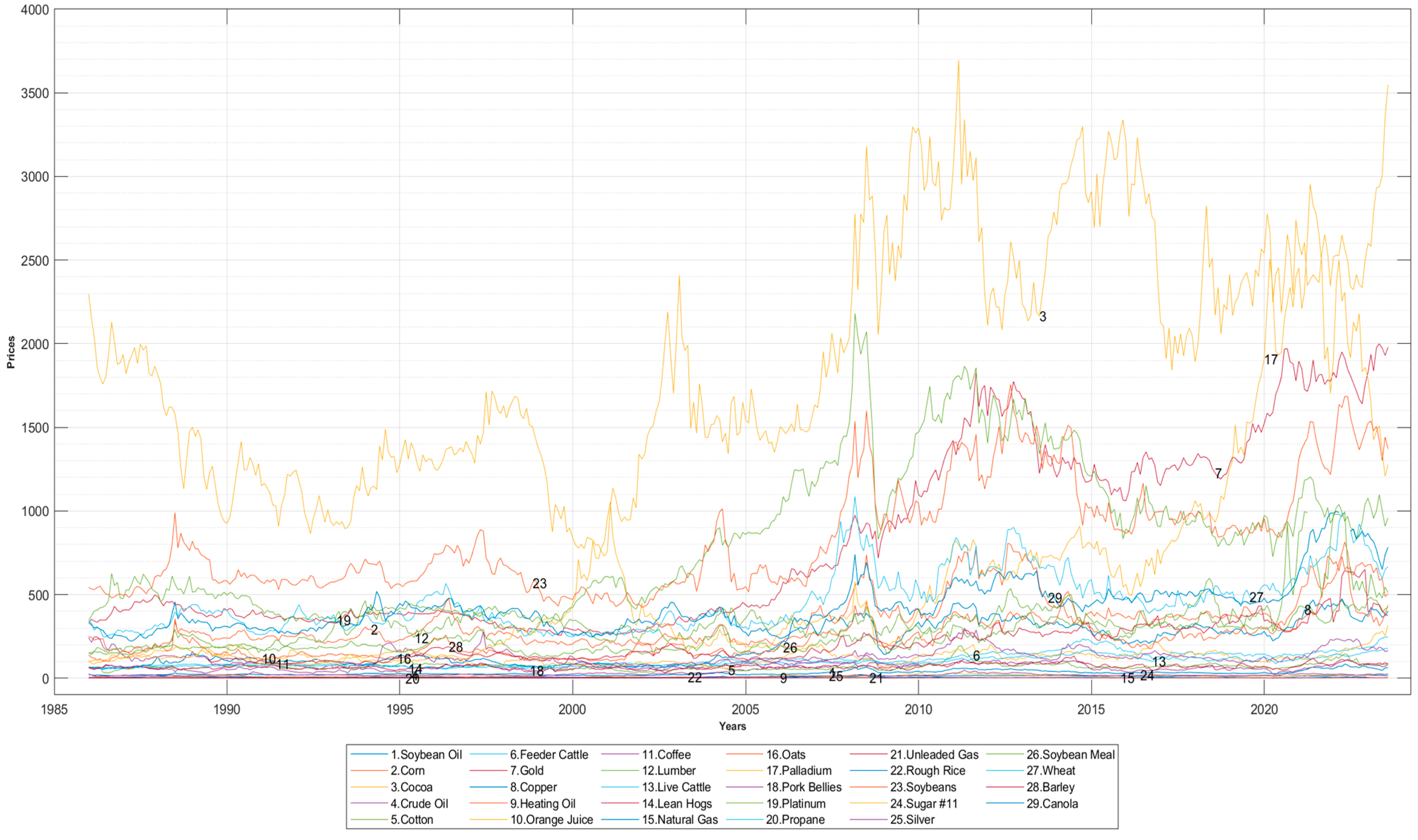Specifically, following the work of [7], we compound the daily returns into cumulative monthly returns, $R_{it}={\sum }_{d=1}^{eom}{r}_{id}$, where eom refers to the end of the month. These return series are then used to create and evaluate the various types of commodity portfolios. Historical prices of individual commodities are plotted in Figure A1, and descriptive statistics of individual commodity returns are presented in

Table A1. Descriptive statistics: individual commodities.

	Mean	CR	SD	Min	Max	Skewness	Kurtosis
Cocoa	−0.5188	−234	8.0165	−28.785	29.6875	0.1243	3.636
Coffee	−0.6278	−283.1206	10.1143	−31.3365	42.6613	0.5551	4.5992
Orange Juice	−0.0147	−6.6269	8.6995	−25.0407	29.4374	0.094	3.617
Sugar #11	0.1362	61.4315	9.0644	−34.5713	34.9778	0.0418	4.3874
Cotton	−0.0184	−8.2789	7.6949	−31.0388	23.8461	−0.1978	4.0266
Lumber	−0.2596	−117.0842	10.8236	−64.2389	46.0502	−0.2975	7.6888
Barley	0.1508	61.9738	6.1868	−21.8238	39.8793	1.0039	7.791
Canola	−0.0223	−10.0427	6.1831	−28.7142	23.3994	−0.4552	5.4765
Corn	−0.4608	−207.8256	7.3697	−25.8788	35.956	0.2619	4.7705
Oats	−0.1975	−89.0938	9.1273	−31.1162	63.8516	0.7947	8.3305
Rough Rice	−0.4947	−219.6356	7.2810	−25.9026	38.6637	0.4419	5.7463
Soybean	0.4025	181.5385	6.5993	−25.3235	20.4418	−0.3283	4.4149
Soybean Meal	0.6729	303.4608	7.3226	−25.576	26.347	0.1317	3.8379
Soybean Oil	−0.1718	−77.4763	7.2582	−29.0301	27.9058	−0.0013	4.6903
Wheat	−0.5632	−253.9907	7.6865	−31.5706	32.0203	0.0689	4.4944
Feeder Cattle	0.0781	35.2143	4.3210	−18.4293	12.9021	−0.3944	3.9947
Live Cattle	0.1114	50.2436	4.0466	−23.6854	14.8651	−0.6142	5.9341
Lean Hugs	−0.6009	−271.0264	7.7993	−36.5695	22.8088	−0.4324	4.3179
Pork Bellies	−0.6014	−173.2065	10.3961	−40.0671	27.1559	−0.1094	3.9253
Crude Oil	−0.0006	−0.2509	10.7254	−77.8608	42.0971	−0.9359	10.2093
Heating Oil	0.2263	102.0503	9.4193	−46.563	29.717	−0.312	4.5338
Unleaded Gas	0.887	400.0487	10.7391	−96.3345	32.1207	−1.7899	18.3911
Natural Gas	−1.2001	−480.0289	13.9262	−42.4143	50.6537	0.0069	3.9244
Propane	0.7635	202.3269	10.9807	−51.1416	53.4501	−0.136	7.5856
Copper	0.5755	259.5598	7.5804	−45.3674	27.8567	−0.4115	6.9585
Gold	0.0782	35.2861	4.4640	−20.4083	14.6615	−0.1063	4.337
Palladium	0.5365	241.9544	9.2337	−41.4469	43.6526	−0.18	5.6968
Platinum	0.2309	104.1423	6.5427	−41.0041	29.2858	−0.615	7.2354
Silver	−0.0028	−1.2552	8.2676	−30.832	30.3172	0.0584	4.2434

(see Appendix A).

The equity return data used to construct the buy-and-hold US domestic reference portfolio were extracted from CRSP. These equity returns are based on a value-weighted index of all NYSE, AMEX, and NASDAQ stocks. The bond index return data for the buy-and-hold US domestic reference portfolio were obtained from Bloomberg, with the returns calculated by Barclays Capital.

3. Commodity Futures Portfolio Construction

After constructing the futures return series, we developed 30 distinct portfolios of commodity futures, categorized by style and performance. This group includes six portfolios following a buy-and-hold strategy, one of which is an equally weighted composite of all included sectors. The five other portfolios are also equally weighted and pertain to specific commodity sectors—foods and fibers, grains and oilseeds, livestock, energy, and precious metals. These are calculated by averaging the monthly return series for each, denoted as $R_{pt}={\sum }_i^n{R}_{it}/n$. The sector-based portfolios are designed to reveal the diverse behaviors of commodity futures returns, underscoring the unique attributes each commodity and sector brings to diversification and risk management. This differentiation suggests that some groups of commodity futures may serve as more effective diversification tools or offer more profitable investment strategies than others. The remaining 24 portfolios are tactically managed, with 21 rebalanced monthly and three, termed net speculation portfolios, rebalanced weekly. These weekly rebalanced portfolios are then compounded to a monthly horizon to support further analysis. The decision for monthly rebalancing aligns with findings that both momentum and term structure strategies yield the highest profits over this timeframe.

The nine momentum portfolios are constructed as follows: at the end of a specified look-back period of L months, all commodities in the sample are ranked in descending order based on their average returns over these L months. The top third of these commodities are placed into a “High” return portfolio, the middle third into a “Medium” return portfolio, and the bottom third into a “Low” return portfolio. These portfolios are then held for H months. We report and analyze results using look-back periods of 1, 3, and 12 months, each paired with a holding period of one month. This methodology follows the approaches of [4,5,7,14,15], assessing the performance of the High, Medium, and Low portfolios over the subsequent H months immediately after the ranking period, without any lag. [15] recommend delaying the measurement of returns by two months post-initial ranking to mitigate issues like non-synchronous trading and bid-ask bounce. However, ref. [7] found that, for commodity futures, delaying or not delaying the measurement after the ranking period does not significantly impact the results; therefore, following the suggestion of [7], we measure the portfolio returns immediately after the ranking period without any lag, creating a single time series of monthly returns for each actively managed trading strategy.

The nine-term structure portfolios are designed differently from the approach outlined by [8]. Inspired by the concepts introduced by [1,3], these strategies aim to capitalize on the term structure of commodity futures prices. This approach is rooted in [16] theory, which suggests that the volatility of futures returns diminishes as the maturity of the contracts extends. Consequently, front-month contracts are most sensitive to immediate changes in supply, demand, and news, whereas contracts further out on the maturity curve are less affected. Additionally, as observed by [8], even contracts of the same commodity with varying maturities can demonstrate significant differences in returns and risks. This indicates that contracts not at the front of the curve may offer distinct investment opportunities due to their different behaviors. We calculate the term structure measures in the following manner:

$${TS}_{i\_j}={\displaystyle \frac{F_{it}-F_{jt}}{F_{it}}}$$

(1)

where ${\mathrm{F}}_{\mathrm{i}\mathrm{t}}$ is the futures price of the nearby contract $\mathrm{i}$ at time $\mathrm{t}$ and ${\mathrm{F}}_{\mathrm{j}\mathrm{t}}$ is the futures price of the next nearby contract $\mathrm{j}$ at time $\mathrm{t}$. For each individual commodity, we utilize Equation (1) at various contract horizons to obtain a daily price difference in percentages. Then, we compute monthly series by averaging daily price differences and use them to sort commodities in descending order. The commodity futures in the top 33% are assigned to a “High” term structure (TS) portfolio, the commodity futures in the middle 33% are assigned to a “Med” TS portfolio, and those commodity futures in the bottom 33% are assigned to a “Low” TS portfolio. The portfolios are then held for one month and rebalanced. For each of the portfolios, the returns for the month, t+1, are calculated using equal weights for all the futures contracts contained within the respective portfolio. This process is repeated to obtain a continuous time series of returns for the portfolios based on the term structure.

The remaining six portfolios employ tactical strategies based on commodity futures and excess speculation. Specifically, for the basis strategy, we sort three portfolios according to the basis of the future (spot price minus futures price) of commodities. For commodities whose spot prices are not available, we use future prices of nearby futures as spot prices and the next nearby future price as the future price to compute the basis. Each month, commodities are ranked in descending order based on the past month’s basis, mirroring the ranking process used in the momentum and term structure strategies. Commodities are then allocated into three portfolios: the top 33% form the “High” basis portfolio, the middle 33% form the “Medium” basis portfolio, and the bottom 33% form the “Low” basis portfolio. Like the earlier portfolios, these are rebalanced monthly. At the end of each month, we calculate the basis for each of the 29 commodity futures, following the methodology of Gorton et al. (2013) [2], where the basis for each commodity, i, is calculated as

$${Basis}_i=\left({\displaystyle \frac{F_{1t}}{F_{2t}}}-1\right)\times {\displaystyle \frac{365}{D_{2t}-D_{1t}}}$$

(2)

where ${\mathrm{F}}_{1\mathrm{t}}$ is the price of the nearest futures contract, ${\mathrm{F}}_{2\mathrm{t}}$ is the price of the next nearby futures contract, and ${\mathrm{D}}_{1\mathrm{t}}$ and ${\mathrm{D}}_{2\mathrm{t}}$ are the number of days before the futures contracts ${\mathrm{F}}_{1\mathrm{t}}$ and ${\mathrm{F}}_{2\mathrm{t}}$ expire, respectively. For each of the portfolios, the returns for the month, t+1, are calculated using equal weights for all the futures contracts contained within their respective portfolio. This process is repeated to obtain a continuous time series of returns for the portfolios based on basis.

In order to construct portfolios based on excess speculators’ positions, we utilize the position of trader data in the US Commodity Futures Trading Commission (CFTC)’s weekly reports. The CFTC data divides traders into commercial hedgers, non-commercial hedgers, and small traders. Those categorized as commercial hedgers participate in the futures market to hedge their inherent commodity price exposure. In contrast, those categorized as speculators hold positions with the intent to profit by anticipating commodity price movements. Following [11,12,17], we calculate excess speculation for each commodity traded in the ith market as follows:

$${\mathrm{Excess\; Speculation}}_{\mathrm{I},\mathrm{t}}=\left\{\begin{array}{c}{\displaystyle \frac{{\mathrm{SS}}_{\mathrm{i}}}{{\mathrm{H}\mathrm{S}}_{\mathrm{I},\mathrm{t}}+{\mathrm{H}\mathrm{L}}_{\mathrm{I},\mathrm{t}}}} \mathrm{if} {\mathrm{HS}}_{\mathrm{I},\mathrm{t}}\ge {\mathrm{HL}}_{\mathrm{I},\mathrm{t}}\\ {\displaystyle \frac{{\mathrm{SL}}_{\mathrm{i}}}{{\mathrm{HS}}_{\mathrm{I},\mathrm{t}}+{\mathrm{HL}}_{\mathrm{I},\mathrm{t}}}} \mathrm{if} {\mathrm{HS}}_{\mathrm{I},\mathrm{t}}<{\mathrm{HL}}_{\mathrm{I},\mathrm{t}}\end{array}\right.$$

(3)

where SS (speculative short) refers to the total non-commercial short position held by all traders, SL (speculative long) refers to the total non-commercial long position held by all traders, HS (hedging short) refers to the total commercial short positions, and HL (hedging long) refers to the total commercial long positions.

Following our prior procedure, each week, t, we rank the commodity futures in descending order based on the past month’s excess speculation positions (${\mathrm{E}\mathrm{S}}_{\mathrm{i},\mathrm{t}}$) and again divide them into three groups. The top one-third of commodities are assigned to a “High” net speculation portfolio, the middle one-third of commodities are assigned to a “Med” net speculation portfolio, and the bottom one-third of commodities are assigned to a “Low” net speculation portfolio. We calculate the portfolio returns by rebalancing weekly and then convert these weekly returns into monthly returns by adding the weekly returns.

4. Buy-and-Hold and Actively Rebalanced Commodity Portfolio Performance

In this section, we present the performance of buy-and-hold and other commodity futures-based portfolios. Before we present descriptive statistics, we provide a density plot of different portfolio returns and a correlation between commodity futures and stock market returns. Figure 1 displays the probability density estimates of returns for selected commodity portfolios, including EWport (an equally weighted portfolio of commodity futures), and portfolios formed based on basis, excess speculation, momentum, and term structure signals (High Basis, High Excess Speculation, High LBP1HP1 Momentum, and HighTS12, respectively). The EWport returns are more concentrated around zero, indicating lower volatility compared to the other portfolios. Actively managed portfolios exhibit broader distributions, suggesting higher risk levels. Portfolios formed on a High Basis and High Excess Speculation information experience negative returns less frequently, as their density peaks are more centered toward positive returns. Overall, while the equally weighted portfolio demonstrates a more stable return distribution, the actively managed portfolios, despite being riskier, show different tendencies for positive returns based on the strategy employed.

4.1. Commodity Portfolio Performance

Table 2. Performance of different styles of commodity portfolios: full sample period.

Portfolios	Mean	p-Value	SD	SR
A: Buy and Hold
Softs	−0.026	0.314	0.159	−0.165
Grains	−0.007	0.820	0.175	−0.037
Livestock	−0.030	0.264	0.165	−0.182
Energy	0.024	0.637	0.301	0.079
Metals	0.034	0.270	0.182	0.185
Ewport	−0.002	0.936	0.119	−0.013
Panel B: Bais
Lowb	−0.116	0.000	0.165	−0.703
Medb	0.007	0.735	0.134	0.056
Highb	0.079	0.002	0.151	0.527
Panel C: Speculation
Lowspec	0.009	0.760	0.169	0.051
Medspec	−0.013	0.588	0.145	−0.089
Highspec	−0.011	0.607	0.131	−0.084
Panel D: Momentum
Lowl1h1	−0.012	0.625	0.151	−0.080
Medl1h1	−0.003	0.877	0.133	−0.026
Highl1h1	0.012	0.650	0.160	0.075
Lowl3h1	−0.020	0.435	0.153	−0.128
Medl3h1	0.000	0.995	0.130	−0.001
Highl3h1	0.017	0.507	0.158	0.110
Lowl12h1	−0.046	0.040	0.139	−0.332
Medl12h1	0.017	0.466	0.139	0.121
Highl12h1	0.032	0.235	0.162	0.199
Panel E: Term Structure
LowTS12	−0.074	0.001	0.143	−0.518
MidTS12	0.004	0.855	0.146	0.030
HighTS12	0.072	0.004	0.147	0.489
LowTS13	−0.038	0.094	0.140	−0.272
MidTS13	0.017	0.464	0.142	0.122
HighTS13	0.014	0.592	0.152	0.089
LowTS14	−0.018	0.415	0.136	−0.134
MidTS14	0.050	0.040	0.142	0.349
HighTS14	−0.039	0.113	0.152	−0.257

Table 2 provides the return performance of the various styles of commodity futures portfolios over the full sample period (31 January 1986 to 31 July 2023). “Mean” represents the average annualized return of the commodity portfolio in percent, “p-val” is the p-value based on two-tailed significance tests for testing the hypothesis of whether the mean return is equal to zero, “SD” is the standard deviation of the portfolio, and “SR” is the Sharpe Ratio.

presents the return performance of various styles of commodity futures portfolios over the period from 31 January 1986 to 31 July 2023. The table is divided into panels based on different portfolio strategies: Buy and Hold (Panel A), Basis (Panel B), Speculation (Panel C), Momentum (Panel D), and Term Structure (Panel E). For each portfolio, the table lists the mean monthly return, the p-value for testing the hypothesis that the mean return is zero, the standard deviation (SD) of the returns, and the Sharpe Ratio (SR), which measures risk-adjusted returns. The returns for buy-and-hold portfolios are mostly negative or close to zero, with low Sharpe Ratios indicating poor risk-adjusted performance. The Energy and Metals portfolios show positive returns, but their p-values suggest these returns are not statistically significant, highlighting the uncertainty and risk associated with these strategies. Panel B presents Basis portfolios, revealing a stark contrast in performance. Highb (High Basis) portfolios exhibit significantly positive returns and a high Sharpe Ratio, indicating good risk-adjusted performance. In contrast, Lowb (Low Basis) portfolios show significantly negative returns and poor risk-adjusted performance. This suggests that basis information can be a critical factor in determining the success of commodity futures portfolios.

Panel C looks at excess speculation portfolios. Lowspec (Low excess Speculation) portfolios display positive returns and a moderate Sharpe Ratio, though the results are not statistically significant. This indicates that while low speculation strategies may offer some potential for positive returns, the associated risks and uncertainties may undermine their overall effectiveness. Panel D covers Momentum portfolios, with a particular focus on high-momentum strategies. High-momentum portfolios, especially Highl3h1 (High long-term momentum), have positive returns and decent Sharpe Ratios, suggesting they may offer better risk-adjusted performance compared to other momentum strategies; however, the varying levels of statistical significance highlight the challenges in consistently leveraging momentum signals for reliable returns. Panel E assesses Term Structure portfolios. HighTS12 portfolios demonstrate significantly positive returns and high Sharpe Ratios, indicating strong performance based on term structure signals. Mid-term structure portfolios also show positive returns and reasonable risk-adjusted performance, underscoring the potential benefits of term structure strategies in commodity futures investing.

4.2. Risk-Adjusted Commodity Portfolio Performance

In order to evaluate the risk-adjusted measures of performance, we calculate risk-adjusted returns for the different portfolios of commodity futures using the autocorrelated regression model of the following form

$$\left.\begin{array}{c}{R}_t=\alpha +X_t\beta +u_t\\ \mathrm{i}\\ u_t={\displaystyle \sum _{i=1}^p{\rho }_i{u}_{t-i}}+v_t+{\displaystyle \sum _{i=1}^q{\delta }_i{v}_{t-i}}\\ \mathrm{i}\\ v_t~iidN\left(0,{\sigma }^2\right)\end{array}\right\}$$

(4)

where ${\mathrm{R}}_{\mathrm{t}}$ is a vector of commodity portfolio return time series, ${\mathrm{X}}_{\mathrm{t}}$ is a matrix of stock and bond market returns, and ${\mathrm{u}}_{\mathrm{t}}$ is a vector of disturbance terms. The regression model is estimated using maximum likelihood. A characteristic advantage of regression models with time series error terms is that a shock at time $\mathrm{t}$, as represented by ${\mathrm{v}}_{\mathrm{t}}$, has an immediate effect on ${\mathrm{R}}_{\mathrm{t}}$ and continues to have an effect at time $\mathrm{t}+1,\mathrm{t}+2,$ etc. Moreover, regression models with time series errors are still able to preserve the sensitivity and interpretation of the regression coefficients; therefore, the autocorrelated regression model helps us to correct for the simple multiple regression model that underestimates returns for some periods and overestimates returns for others. We regress the monthly returns of the various commodity portfolios on the CRSP value-weighted market index and the Barclays Capital U.S. Aggregate Bond index to obtain the risk-adjusted returns. The risk-adjusted return results from the model in (4) are presented in Table 2.

Table 3. Risk-adjusted returns of different portfolios.

Portfolios	Alphas	p-Value	Stock	p-Value	Bond	p-Value
A: Buy and Hold
Softs	−0.003	0.946	0.262	0.000	−0.321	0.965
Grains	−0.001	0.701	0.192	0.000	−0.216	0.854
Livestock	−0.003	0.863	0.124	0.003	−0.241	0.890
Energy	0.000	0.473	0.378	0.000	−0.423	0.891
Metals	0.000	0.510	0.326	0.000	−0.054	0.604
Ewport	−0.001	0.772	0.247	0.000	−0.246	0.963
Panel B: Basis
Lowb	−0.012	1.000	0.317	0.000	−0.324	0.962
Medb	0.000	0.496	0.227	0.000	−0.351	0.987
Highb	0.005	0.014	0.213	0.000	−0.192	0.875
Panel C: Speculation
Lowspec	0.000	0.514	0.178	0.000	−0.196	0.854
Medspec	−0.003	0.903	0.182	0.000	−0.004	0.510
Highspec	−0.002	0.806	0.115	0.000	−0.103	0.765
Panel D: Momentum
Lowl1h1	−0.003	0.881	0.323	0.000	−0.321	0.960
Medl1h1	−0.002	0.780	0.237	0.000	−0.227	0.921
Highl1h1	0.000	0.425	0.166	0.000	−0.236	0.909
Lowl3h1	−0.003	0.904	0.282	0.000	−0.307	0.959
Medl3h1	−0.001	0.659	0.229	0.000	−0.305	0.980
Highl3h1	0.000	0.460	0.214	0.000	−0.185	0.824
Lowl12h1	−0.005	0.990	0.240	0.000	−0.359	0.989
Medl12h1	0.000	0.484	0.200	0.000	−0.130	0.800
Highl12h1	0.001	0.337	0.290	0.000	−0.251	0.916
Panel E: Term Structure
LowTS12	−0.008	1.000	0.265	0.000	−0.167	0.857
MidTS12	−0.002	0.751	0.244	0.000	−0.072	0.663
HighTS12	0.006	0.005	0.243	0.000	−0.506	0.999
LowTS13	−0.005	0.981	0.236	0.000	−0.169	0.847
MidTS13	−0.001	0.640	0.243	0.000	−0.023	0.560
HighTS13	0.001	0.349	0.272	0.000	−0.541	0.999
LowTS14	−0.002	0.880	0.185	0.000	−0.183	0.863
MidTS14	0.002	0.233	0.285	0.000	−0.056	0.641
HighTS14	−0.004	0.956	0.292	0.000	−0.442	0.995

Table 3 provides the risk-adjusted return performance of the various styles of commodity futures portfolios over the full sample period (31 January 1986 to 31 July 2023) using the autocorrelated regression model of the form stated in Equation (4). “Alpha” represents the average annualized risk-adjusted return of the commodity portfolio, “p-val” is the p-value based on two-tailed significance tests for testing the hypothesis of whether the mean return is equal to zero, “stock” is the CRSP value-weighted market index, and “bond” is the Barclays Capital U.S. Aggregate Bond index. p-values that are less than 5% are shaded with gray color.

provides the risk-adjusted performance of various commodity portfolios. For the buy-and-hold portfolios, the results reveal that the alphas, which represent the average annualized risk-adjusted returns, are generally negative and not statistically significant. This implies that these portfolios do not consistently provide returns above what would be expected after adjusting for risk. The stock market coefficients are positive and highly significant across all buy-and-hold portfolios, indicating a strong positive correlation with the stock market. This suggests that as stock market returns increase, so do the returns of these commodity portfolios. Conversely, the bond market coefficients are negative but not significant, suggesting a weaker and inconsistent relationship with bond market returns.

Basis portfolios also show mixed results. The Lowb and Medb portfolios show no significant alphas, whereas the Highb portfolio exhibits a positive and significant alpha. This indicates that the Highb portfolio potentially offers excess returns after adjusting for risk. Similar to the buy and hold portfolios, all Basis portfolios display positive and significant stock market coefficients, reinforcing the strong positive correlation with stock market returns. The bond market coefficients remain negative and not significant, indicating a minimal impact of bond market returns on these portfolios. The portfolios based on excess speculation also demonstrate a lack of significant alphas, indicating no consistent excess returns. The stock market coefficients are positive and significant across all speculation-based portfolios, underscoring the persistent positive relationship with stock market returns. The bond market coefficients continue to be negative and insignificant, further suggesting that bond market movements do not substantially influence these portfolios.

In the case of Momentum portfolios, the results consistently show non-significant alphas, signifying no consistent risk-adjusted excess returns. The positive and significant stock market coefficients reaffirm the strong link between these portfolios and the stock market. The bond market coefficients, while negative, do not show statistical significance, indicating an insignificant relationship with bond returns. The term structure portfolios present a similar pattern, with most alphas being non-significant, except for the HighTS12 portfolio, which has a positive and significant alpha. This suggests that the HighTS12 portfolio might deliver excess returns after risk adjustment. As with the other portfolios, the stock market coefficients are positive and significant, highlighting the robust correlation with stock market performance. The bond market coefficients remain negative and insignificant, suggesting a weak and inconsistent relationship with bond returns.

Overall, these findings suggest that commodity portfolios, in general, are significantly influenced by stock market returns but not by bond market returns. The lack of significant alphas in most portfolios indicates that these commodity portfolios do not consistently generate risk-adjusted excess returns. This is consistent with the financialization of the commodity futures market, which has led to increased correlations with traditional financial assets, particularly stocks. The few exceptions where portfolios do show significant alphas indicate that certain strategies may offer opportunities for excess returns, but these are not widespread across all portfolio types.

We also evaluate the performance of these two portfolios by dividing our samples into two sub-periods based on the argument of financialization, as the period after 2003 marks the financialization of commodity markets.

Table 4. Performance of different styles of commodity portfolios: pre-2003 and post-2003 sample periods.

	Period: 01/31/1986 to 10/31/2003				Period: 11/31/2003 to 07/31/2023				Difference in Mean
Portfolios	Mean	p-Value	SD	SR	Mean	p-Value	SD	SR	Test (p-Value)
A: Buy and Hold
Softs	−0.040	0.207	0.131	−0.303	−0.014	0.729	0.180	−0.078	0.308
Grains	−0.029	0.449	0.162	−0.182	0.015	0.722	0.187	0.081	0.221
Livestock	0.001	0.986	0.173	0.004	−0.052	0.135	0.157	−0.329	0.163
Energy	0.075	0.299	0.286	0.262	−0.025	0.721	0.311	−0.080	0.163
Metals	0.010	0.787	0.143	0.066	0.055	0.261	0.210	0.260	0.235
Ewport	−0.004	0.851	0.088	−0.046	0.001	0.975	0.140	0.007	0.450
Panel B: Bais
Lowb	−0.082	0.003	0.117	−0.698	−0.144	0.001	0.197	−0.734	0.102
Medb	0.002	0.943	0.100	0.017	0.012	0.734	0.157	0.077	0.409
Highb	0.082	0.013	0.130	0.632	0.079	0.042	0.167	0.476	0.479
Panel C: Speculation
Lowspec	0.002	0.961	0.151	0.012	0.013	0.754	0.184	0.071	0.421
Medspec	−0.034	0.198	0.110	−0.310	0.003	0.937	0.169	0.018	0.217
Highspec	0.000	0.996	0.124	−0.001	−0.022	0.462	0.137	−0.164	0.302
Panel D: Momentum
Lowl1h1	−0.030	0.326	0.125	−0.237	0.005	0.906	0.170	0.027	0.245
Medl1h1	−0.014	0.570	0.104	−0.138	0.006	0.872	0.154	0.036	0.326
Highl1h1	0.037	0.301	0.144	0.257	−0.008	0.827	0.174	−0.049	0.200
Lowl3h1	−0.008	0.788	0.122	−0.066	−0.027	0.490	0.176	−0.154	0.352
Medl3h1	−0.010	0.691	0.101	−0.097	0.009	0.784	0.150	0.062	0.329
Highl3h1	0.006	0.850	0.140	0.046	0.024	0.536	0.172	0.141	0.369
Lowl12h1	−0.074	0.012	0.124	−0.598	−0.022	0.502	0.150	−0.150	0.120
Medl12h1	0.027	0.307	0.105	0.253	0.010	0.786	0.162	0.061	0.361
Highl12h1	0.048	0.169	0.139	0.344	0.020	0.618	0.180	0.114	0.311
Panel E: Term Structure
LowTS12	−0.066	0.011	0.108	−0.606	−0.082	0.025	0.168	−0.487	0.358
MidTS12	−0.001	0.976	0.116	−0.007	0.010	0.796	0.168	0.059	0.413
HighTS12	0.065	0.044	0.127	0.509	0.078	0.039	0.162	0.484	0.396
LowTS13	−0.040	0.140	0.113	−0.355	−0.037	0.295	0.161	−0.232	0.475
MidTS13	0.019	0.468	0.107	0.179	0.017	0.644	0.166	0.105	0.485
HighTS13	0.008	0.806	0.131	0.060	0.019	0.623	0.168	0.112	0.415
LowTS14	−0.002	0.952	0.115	−0.015	−0.032	0.338	0.153	−0.213	0.245
MidTS14	0.034	0.195	0.107	0.322	0.064	0.098	0.167	0.385	0.274
HighTS14	−0.046	0.132	0.127	−0.361	−0.033	0.381	0.172	−0.195	0.399

Table 4 presents the return performance of various styles of commodity futures portfolios over two sub-sample periods: 31 January 1986 to 31 October 2003, and 31 November 2003 to 31 July 2023. The “Mean” column represents the average annualized return of the commodity portfolio. The “p-value” column provides the p-value from two-tailed significance tests to determine whether the mean return is significantly different from zero. “SD” denotes the standard deviation of the portfolio, and “SR” represents the Sharpe Ratio. The final column shows the p-values for the differences in mean returns between these two periods.

illustrates the performance of various commodity futures portfolios over two distinct periods: from 31 January 1986 to 31 October 2003, and from 31 November 2003 to 31 July 2023. Each portfolio’s performance is analyzed using key metrics such as mean return, standard deviation (SD), and Sharpe Ratio (SR). The table also includes p-values for the mean returns and the differences in mean returns between the two periods, providing insights into the statistical significance of the observed changes.

Similar to the findings of the analysis for the entire period, the average returns of all portfolios are not significantly different from zero in both periods, as indicated by the p-values being higher than five percent. This suggests that, on average, the commodity futures portfolios did not generate substantial positive or negative returns in either the pre-financialization period or the financialization period; moreover, the differences in mean returns between the two periods for the various commodity portfolios were mostly insignificant. This lack of significant differences highlights the stability of these portfolios across both periods, indicating that they did not undergo substantial performance shifts; thus, the commodity portfolios provided a consistent return profile over time, maintaining similar performance in both the financialization and pre-financialization periods.

5. Conclusions

In this paper, we have analyzed the return performance of both buy-and-hold and tactical portfolios of commodity futures. By examining a comprehensive dataset spanning from 31 January 1986 to 31 July 2023, we constructed and evaluated 30 distinct portfolios categorized by style and performance. The primary objective was to determine whether these commodity portfolios provide meaningful diversification benefits when included in traditional equity and bond portfolios.

The findings from our analysis reveal several critical insights. Buy-and-hold portfolios generally exhibit poor risk-adjusted performance, with returns often close to zero or negative, as indicated by low Sharpe Ratios. In contrast, tactical portfolios, particularly those based on basis and momentum strategies, demonstrate significantly positive returns and higher Sharpe Ratios. Similarly, high-term structure portfolios also exhibit strong performance.

Overall, this study underscores the importance of tactical investment strategies in enhancing portfolio performance through commodity futures; however, it also highlights the need for investors to adapt to the evolving market conditions that influence the effectiveness of these diversification strategies. Future research should focus on further understanding the implications of increased market integration and financial innovation on the risk and return characteristics of commodity futures.