A Unified Benchmark of Machine Learning and Deep Neural Networks for Tennis Match Prediction

Abstract

Tennis match prediction has been studied extensively, yet the literature offers no controlled comparison of Elo ratings, classical machine learning, and deep neural networks under identical experimental conditions, leaving practitioners without clear guidance on model selection. We address this gap with a unified empirical study on 133,138 professional men’s tennis matches from the Association of Tennis Professionals tour (1968–2024). Four approaches are evaluated on the same temporally split data with a common 16-feature set and an aligned evaluation protocol: an enhanced Elo rating system, ten classical machine learning algorithms, seventeen deep neural network configurations spanning 207,000 to 21,000,000 parameters, and a hybrid Elo–machine learning (ELO-ML) approach that augments classical learners with three Elo-derived features. A tuned Elo baseline alone reaches 65.87% accuracy, the best of ten classical machine learning algorithms reaches 66.30%, seventeen deep neural network configurations cluster at 66.15–66.22%, and the hybrid ELO-ML approach reaches 67.52% (McNemar’s test, $p<0.001$ for all ELO-ML pairwise comparisons). All four approaches sit within a 1.65 pp band whose upper edge lies below the 70–72% accuracy commonly cited for bookmaker odds, indicating that pre-match prediction under universally available features is a difficult task in which Elo alone already captures most of the predictable signal and algorithmic sophistication adds only marginal headroom. Deep neural networks deliver substantially better probability calibration than the other approaches (Expected Calibration Error 0.0077 vs. 0.0142). Model capacity exhibits sharply diminishing returns: all seventeen network configurations, spanning a 100-fold range in parameter count (207,000 to 21,000,000), fall within a 0.07 pp accuracy band. The study establishes a controlled benchmark for tour-level tennis prediction, quantifies how narrow the headroom above Elo actually is, provides modest but consistent empirical support for the statistically enhanced learning framework, and supplies deployment-ready operating points for sports analytics practitioners.

1. Introduction

The prediction of sports outcomes has evolved from informal expert intuition into a quantitative discipline grounded in statistical and computational methods. Tennis is a particularly attractive domain for predictive analytics: it has a structured scoring system, decades of well-curated match records, and clear commercial relevance for analysts, broadcasters, and risk-management applications in regulated betting markets [1,2,3,4]. Over the past two decades, the methodological toolkit has expanded from ranking-based heuristics and point-based probabilistic models to ensemble learners and, more recently, deep neural networks [5,6,7,8,9,10,11].

Despite this expanded toolkit, the literature offers conflicting evidence on which family of methods is most effective for pre-match prediction. Some studies report neural-network gains over classical baselines [3], while others observe negligible differences between deep models and well-tuned tree ensembles when given the same input features [12,13]. Recent advances in tabular deep learning—including attention-based architectures such as TabTransformer [14] and FT-Transformer [15], as well as hybrid approaches such as TabNet [16]—have renewed interest in whether architectural innovation can close the gap with gradient-boosted trees on structured data; however, comprehensive evaluations suggest these gains are task- and dataset-dependent and do not consistently generalize [17]. A second open question concerns the role of feature engineering relative to representation learning. Recent work argues that statistically derived features—most prominently Elo ratings—substantially boost any underlying learner, an idea formalized by Felice et al. [18] as statistically enhanced learning (SEL) and partially supported by Grand-Slam-only results from Buhamra et al. [19]. A third unresolved question is the relationship between model capacity and accuracy on structured sports data: while computer vision and language modeling have repeatedly demonstrated benefits from scale, tennis datasets are small and low-dimensional, and the larger-is-better assumption has not been empirically tested for this setting.

The core obstacle to settling these debates is methodological heterogeneity. Different studies use different time windows, tournament tiers, feature sets, and evaluation protocols, so cross-paper comparisons cannot reliably attribute performance differences to modeling choices rather than data choices [1]. As a result, practitioners have no controlled benchmark to consult when selecting an approach for tennis or for analogous structured-tabular sports prediction tasks.

This paper closes that gap with a unified empirical study. We evaluate four distinct modeling paradigms on identical data, with a single feature set, identical temporal train–validation–test splits, and a common suite of metrics. Specifically, we compare (i) an enhanced Elo rating system with surface-specific ratings, tournament-level K-factors, inactivity decay, and margin-of-victory scaling; (ii) ten classical machine learning algorithms spanning linear, probabilistic, instance-based, single-tree, bagging, and boosting families; (iii) seventeen deep neural network configurations covering plain and residual multilayer perceptrons with model capacity ranging from approximately 207,000 to 21,000,000 parameters; and (iv) a hybrid ELO-ML approach that augments classical learners with three Elo-derived features, operationalizing the SEL framework on tour-level data.

We address the following research questions: (RQ1) How do classical machine learning methods compare to deep neural networks in predictive accuracy for pre-match tennis outcome prediction? (RQ2) How does deep network capacity affect predictive performance for this structured-data task? (RQ3) Does integrating Elo-derived domain-informed features into machine learning models yield consistent gains across algorithm families? (RQ4) Do the approaches differ in probability calibration, beyond classification accuracy?

The study makes four contributions.Methodologically, we deliver the first head-to-head comparison of Elo ratings, classical machine learning, deep neural networks, and a hybrid ELO-ML approach under identical experimental conditions on a tour-wide ATP dataset spanning more than five decades. Empirically, the controlled comparison quantifies how narrow the headroom above Elo actually is for this task: a tuned Elo baseline alone reaches 65.87%, the best of ten classical ML algorithms reaches 66.30%, and seventeen deep network configurations span only a 0.07 pp accuracy band from 66.15% to 66.22%—all sitting within a 1.65 pp envelope whose upper edge remains below the 70–72% accuracy commonly cited for bookmaker odds. The seventeen-configuration architecture sweep further reveals a sharp performance plateau in which a 100-fold increase in parameter count yields essentially zero accuracy improvement. Together these results indicate that pre-match prediction is fundamentally constrained by feature richness rather than by model class. As a secondary, framework-level finding, augmenting classical learners with three Elo-derived features (ELO-ML) yields a consistent +1.57–1.65 percentage point (pp) uplift across three algorithm families ($p<0.001$ by McNemar’s test), with the best ELO-ML model reaching 67.52%; while statistically significant and cross-family consistent, the gain is modest in absolute terms and is best interpreted as a useful augmentation rather than a categorical performance breakthrough, providing clean empirical evidence on tour-level data for the SEL framework. Practically, the results give deployment-ready benchmarks: the best high-accuracy model trains in 87 s with a 142 MB memory footprint, the most efficient near-best model trains in 23 s with 18 MB, and a 207,000-parameter neural network matches the accuracy of a 21,000,000-parameter one.

The remainder of the paper is organized as follows. Section 2 describes the dataset, the four modeling approaches, and the evaluation protocol. Section 3 presents the experimental results. Section 4 interprets the findings, compares them with prior work, and discusses implications and limitations. Section 5 concludes.

2. Materials and Methods

This section describes the dataset and preprocessing pipeline (Section 2.1), the Elo rating system (Section 2.2), the classical machine learning approach (Section 2.3), the deep neural network architectures (Section 2.4), the hybrid ELO-ML approach (Section 2.5), and the evaluation metrics and statistical testing protocol (Section 2.6).

2.1. Dataset and Preprocessing

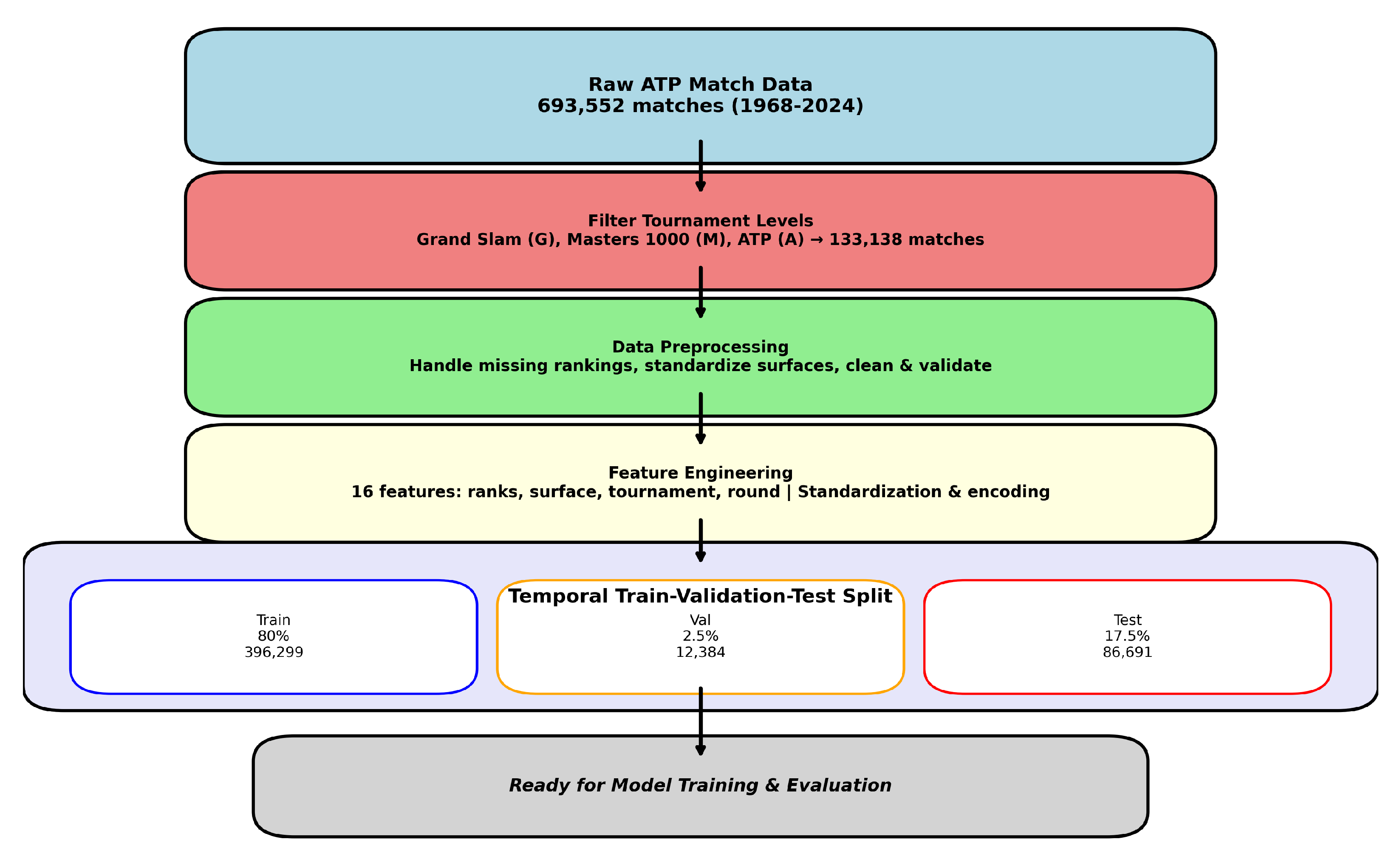
The dataset consists of professional men’s tennis match records from the Jeff Sackmann ATP database [20], containing 693,552 matches from August 1968 to November 2024. To focus the analysis on elite competition where match statistics are most consistently recorded, the raw data were filtered to retain only Grand Slam (G), Masters 1000 (M), and ATP 250 and 500 (A) tournaments, yielding 133,138 matches. Court surfaces were standardized to four categories (hard, clay, grass, carpet); missing ATP rankings, which occur primarily for newly professional or returning players, were forward-filled from the most recent known value for each player, with a default rank of 300 assigned to players never previously ranked or appearing for the first time in the dataset. Rows with missing target labels (less than 0.5% of the filtered dataset) were removed.

Each match was represented symmetrically from both players’ perspectives, producing 266,276 player-match observations and ensuring that models learn perspective-invariant patterns rather than artifacts of the ordering of player A and player B. The dataset was split chronologically into training (80%, 396,299 observations), validation (2.5%, 12,384 observations), and test (17.5%, 86,691 observations) partitions. The temporal split mirrors real-world deployment, in which a model trained on historical data must predict future matches it has never seen; it also rules out information leakage from future results into model selection. All preprocessing steps—including one-hot encoding for categorical variables and z-score standardization for continuous features—were fit exclusively on the training partition and then applied without modification to validation and test data.

Table 1. Dataset summary statistics.

Attribute	Value
Total matches (raw)	693,552
Total matches (filtered)	133,138
Player-match observations	266,276
Date range	29 August 1968 to 4 November 2024
Tournament levels included	G, M, A
Unique players	1707
Training observations	396,299
Validation observations	12,384
Test observations	86,691

summarizes the dataset, and Figure 1 illustrates the full preprocessing pipeline.

A common 16-feature input vector was used for all machine learning approaches, derived from standard match metadata available across the full date range: each player’s ATP rank, their rank difference, log-transformed ranks, and absolute log rank difference, one-hot encoded surface (hard, clay, grass, carpet), encoded tournament level, encoded round, best-of format, draw size, and calendar year. This deliberately compact feature set ensures comparability across the entire 56-year span (where detailed serve and return statistics are unavailable for much of the older data) and reflects the realistic information available for pre-match prediction at most events.

To improve robustness and expand effective training-set size, two augmentation strategies were applied during training only: symmetric representation of every match (which doubles the number of training observations) and Gaussian noise injection on continuous features with standard deviation equal to 1% of each feature’s standard deviation [21]. Ablation indicated that noise injection contributed an additional 0.2–0.3 pp of accuracy across most algorithms, with the largest gains observed for the models most susceptible to overfitting.

2.2. Elo Rating System

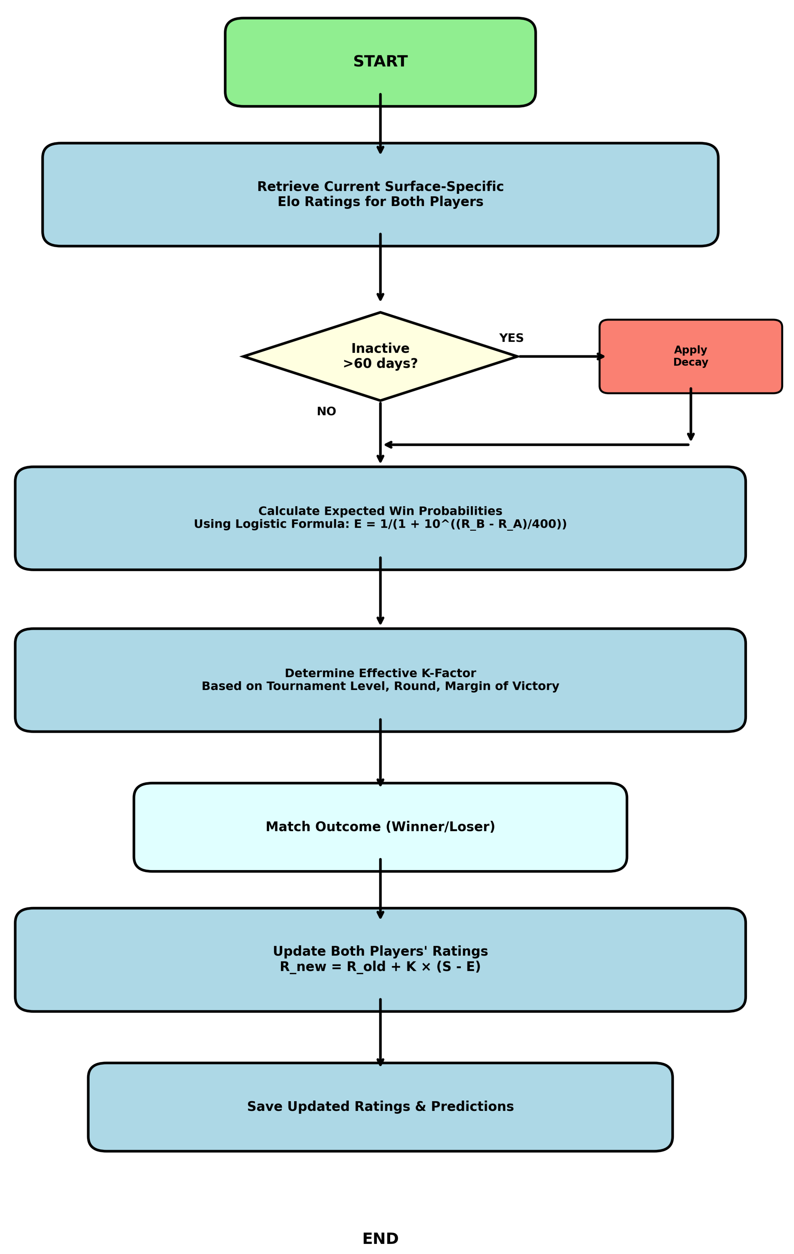
The Elo rating system [22] provides a dynamic measure of player skill that updates continuously after each match. The standard Elo update equation is

$$R_{\mathrm{new}}=R_{\mathrm{old}}+K(S-E),E_A={\displaystyle \frac{1}{1+{10}^{(R_B-R_A)/400}}},$$

(1)

where $R_{\mathrm{old}}$ is the player’s rating before the match, K is the rating-update step size, $S\in \{0,1\}$ is the actual outcome from the player’s perspective, and E is the expected score computed via the logistic function of the rating difference. A 400-point rating gap corresponds to roughly a 91% expected win probability for the higher-rated player.

Our implementation augments the base formula with several professional-tennis-specific enhancements [23]:

• Surface-specific ratings. Each player maintains four independent ratings, one per surface, all initialized at 1500. A match outcome updates only the relevant surface rating, allowing the system to capture surface specialization.
• Tournament-level K-factors. K is set to 48 for Grand Slams, 36 for Masters 1000 events, and 32 for ATP 250 and 500 events, reflecting the differing prestige and information content of each tier.
• Round multipliers. The effective K scales by 1.25 for finals and progressively down to 0.90 for early rounds.
• Inactivity decay. Ratings decay by 0.5 points per day after 60 days of inactivity, capped at a 200-point total decay, preventing inflated ratings for inactive players.
• Margin-of-victory adjustment.The effective outcome S is scaled by margin of victory (e.g., straight-sets vs. five-set wins), giving additional credit for dominant wins [23].

All ratings were computed chronologically across the full dataset before any model training, ensuring that the rating used as a feature for any match reflects only information available prior to that match. This was formally verified by an independent recomputation script: stored Elo features matched strict pre-match recomputed values with zero numerical deviation (max absolute difference $<{10}^{-6}$) across all observations; a deliberately biased variant that updated ratings before capture produced mean absolute deviations of approximately 16 Elo points, confirming the sensitivity of the test. Figure 2 illustrates the update process.

2.3. Classical Machine Learning Approach

Ten algorithms were evaluated, spanning a representative cross-section of classical machine learning: Logistic Regression, Ridge Classifier, Gaussian Naive Bayes, k-Nearest Neighbors, Decision Tree, Random Forest, Extra Trees, Gradient Boosting, Histogram-Based Gradient Boosting, and AdaBoost. All algorithms were implemented in scikit-learn 1.3 [24]. This selection covers linear, probabilistic, instance-based, single-tree, bagging, and boosting families and therefore enables broad conclusions about the classical-ML envelope of performance for this task.

Hyperparameter optimization was performed within the training partition only, via grid search with 5-fold stratified cross-validation. The hyperparameter spaces explored for the top-performing algorithms were: for Random Forest, 100–500 trees, maximum depth 10–30, and minimum samples per split 2–10; for Gradient Boosting and Histogram-Based Gradient Boosting, 100–300 estimators, learning rate 0.01–0.20, and maximum depth 3–9; for Logistic Regression, regularization strength C over $\{{10}^{-3},\dots ,{10}^2\}$ with both $L_1$ and $L_2$ penalties; for AdaBoost, 50–300 estimators and learning rate 0.01–1.0. The single best configuration per algorithm (by mean cross-validation accuracy) was retrained on the full training set and evaluated once on the held-out test set, with no further tuning. The validation partition (2.5%) was not used during classical machine learning hyperparameter selection; it was reserved exclusively for early stopping in the deep neural network experiments (Section 2.4).

2.4. Deep Neural Network Architectures

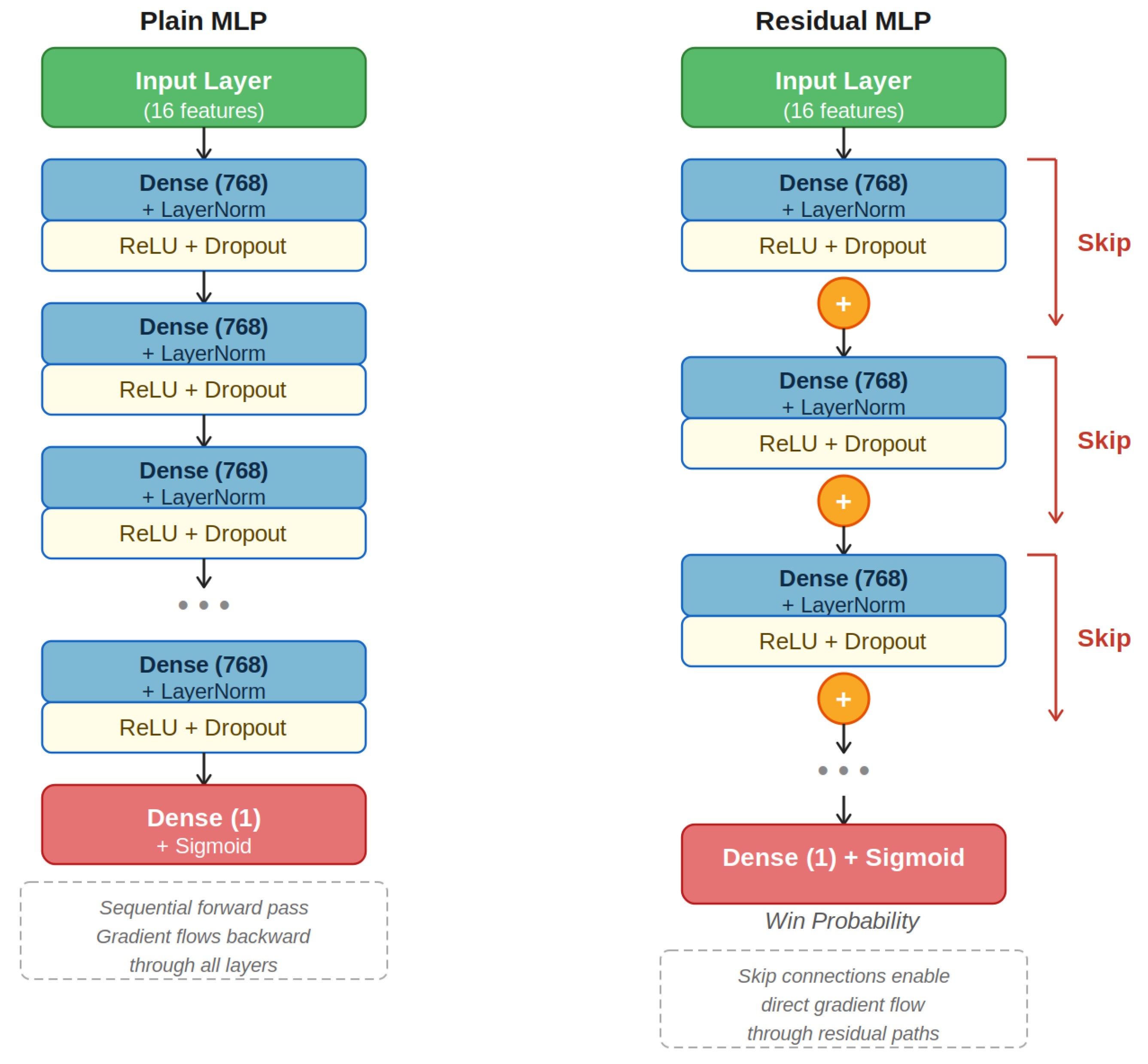
Deep neural network experiments focused on multilayer perceptron (MLP) architectures, which are the standard deep learning baseline for structured tabular data and afford the most direct comparison with the classical machine learning models above. Two architectural variants were evaluated: a plain MLP, in which each block applies a linear transformation followed by layer normalization, dropout, and a Rectified Linear Unit (ReLU) activation; and a residual MLP, which adds skip connections [25] that bypass pairs of layers to improve gradient flow in deeper networks. The plain block update is

$$h^{\left(l\right)}=\mathrm{ReLU}\left(\mathrm{LayerNorm}\left(W^{\left(l\right)}·\mathrm{Dropout}\left(h^{(l-1)}\right)+b^{\left(l\right)}\right)\right),$$

(2)

and the residual variant adds the input of the block to its output before activation. Figure 3 illustrates both variants.

To systematically probe the effect of model capacity, four target size tiers were tested—approximately 207,000 (tiny), 1,300,000 (small), 9,500,000 (medium), and 21,000,000 (large) parameters—achieved by varying hidden-layer dimensionality (512, 768, or 1024 units), depth (6, 8, or 12 hidden layers), and architecture type (plain or residual). Additional hyperparameters varied across configurations were dropout rate (0.00–0.35), $L_2$ weight decay (0.0–0.001), and batch size (64–512). In total, 17 configurations were trained and evaluated. The configuration dimensions are summarized in

Table 2. Summary of deep neural network configuration dimensions explored.

Dimension	Values Explored
Architecture type	Plain, Residual
Number of hidden layers	6, 8, 12
Hidden layer dimensionality	512, 768, 1024
Dropout rate	0.00, 0.10, 0.15, 0.20, 0.25, 0.30, 0.35
$L_2$ weight decay	0.0, 0.0001, 0.0005, 0.001
Batch size	64, 128, 256, 512
Approximate parameter count	207 K, 1.3 M, 9.5 M, 21 M

.

All models were implemented in PyTorch 2.0.1 and trained on an NVIDIA A100 GPU. Optimization used AdamW [26] with a cosine annealing learning-rate schedule from ${10}^{-3}$ to ${10}^{-6}$, a binary cross-entropy loss, and early stopping (patience of 20 epochs) on the validation set, up to a maximum of 200 epochs. Training times ranged from approximately 130 s for the tiny configuration to over 7200 s for the large configuration on the same GPU.

2.5. Hybrid ELO-ML Combined Approach

The ELO-ML approach operationalizes the SEL framework [18] by augmenting the 16-feature classical machine learning input with three Elo-derived features: the Elo rating of player A, the Elo rating of player B, and their difference. Elo ratings were taken from the system described in Section 2.2, computed chronologically to prevent any leakage of future match outcomes into training features.

Three algorithms were evaluated under this approach—Logistic Regression, Ridge Classifier, and AdaBoost—chosen to represent a linear probabilistic classifier, a linear discriminative classifier, and a boosting ensemble. Gradient boosting variants (Histogram-Based Gradient Boosting, Gradient Boosting) were intentionally excluded from this evaluation: their internal tree-splitting mechanism already exploits a monotonic rank-based signal directly from the input features, making it difficult to isolate the marginal contribution of the Elo augmentation cleanly. The three selected algorithms provide a cleaner test of whether the SEL benefit is consistent across structurally distinct algorithm families.

2.6. Evaluation Metrics and Statistical Testing

All models were assessed using a consistent suite of metrics spanning classification, probabilistic prediction, and calibration. Classification metrics included accuracy, precision, recall, and $F_1$ score. Probabilistic metrics included the area under the Receiver Operating Characteristic curve (ROC-AUC) [27], log loss, and Brier score [28].

Probability calibration was assessed using the Expected Calibration Error (ECE) [29]:

$$\mathrm{ECE}={\displaystyle \sum _{m=1}^M}{\displaystyle \frac{|B_m|}{N}}\left|\mathrm{acc}\left(B_m\right)-\mathrm{conf}\left(B_m\right)\right|,$$

(3)

where M is the number of probability bins, $B_m$ is the set of predictions falling into bin m, N is the total number of predictions, $\mathrm{acc}\left(B_m\right)$ is the observed accuracy within the bin, and $\mathrm{conf}\left(B_m\right)$ is the mean predicted confidence within the bin. ECE was computed using 10 equal-width bins over $[0,1]$. A lower ECE indicates better calibration: when a well-calibrated model predicts a 70% win probability, the empirical win rate among such predictions is close to 70%.

Statistical significance of pairwise model differences was assessed via McNemar’s test [30], which is appropriate when comparing two classifiers evaluated on the same test set. All test set evaluations were one-shot: every model was trained and tuned only on the training partition (with cross-validation contained entirely within it), and the held-out test set was used exactly once per model, after all design choices had been finalized.

3. Results

This section reports the experimental results for each of the four approaches and a unified comparison across them. Section 3.1 provides an overall performance summary. Section 3.2, Section 3.3, Section 3.4 and Section 3.5 report the per-approach results. Section 3.6 integrates the findings via head-to-head accuracy, calibration, efficiency, and statistical significance analyses.

3.1. Overall Performance Summary

Table 3. Overall performance of the best model from each approach on the held-out test set.

Approach	Accuracy (%)	ROC-AUC	Brier Score
Elo Rating System	65.87	0.7245	0.2120
Classical ML (Best: Hist. Gradient Boosting)	66.30	0.7253	0.2101
Deep Neural Network (Best: Small-Residual)	66.22	0.7250	0.2098
ELO-ML Combined (Best: AdaBoost)	67.52	0.7305	0.2071

summarizes the best model from each approach on the held-out test set. A clear and consistent performance hierarchy emerges: ELO-ML (67.52%) > classical machine learning (66.30%) > deep neural networks (66.22%) > Elo baseline (65.87%). ROC-AUC tracks accuracy, with the ELO-ML approach achieving the highest discriminative ability at 0.7305 and the Elo baseline the lowest at 0.7245.

3.2. Elo Rating System Results

The Elo rating system achieved 65.87% accuracy and a ROC-AUC of 0.7245 on the full test set, establishing a strong domain-informed baseline. Surface-conditioned analysis revealed meaningful per-surface variation: 67.3% accuracy on clay (the most predictable surface, where physical endurance and baseline consistency tend to favor higher-rated players), 66.1% on hard, 65.8% on carpet, and 64.2% on grass (the smallest surface subsample and the most upset-prone, given the fast and unpredictable conditions). The system produced well-calibrated predictions for rating differences within $\pm 200$ points, with mild overconfidence emerging only for rating differences exceeding 300 points.

3.3. Classical Machine Learning Results

Table 4. Classical machine learning algorithm performance on the held-out test set, ranked by accuracy.

Algorithm	Accuracy (%)	ROC-AUC	F1 Score	Brier Score
Histogram Gradient Boosting	66.30	0.7253	0.6628	0.2101
Gradient Boosting	66.28	0.7251	0.6626	0.2103
Random Forest	66.15	0.7242	0.6613	0.2108
Extra Trees	65.98	0.7235	0.6596	0.2115
AdaBoost	65.87	0.7228	0.6585	0.2119
Logistic Regression	65.82	0.7223	0.6580	0.2122
Ridge Classifier	65.81	0.7222	0.6579	0.2123
Decision Tree	63.45	0.6845	0.6342	0.2298
k-Nearest Neighbors	62.87	0.6789	0.6285	0.2345
Naive Bayes	61.23	0.6654	0.6119	0.2421

summarizes the performance of all ten classical machine learning algorithms on the test set, ranked by accuracy. A clear hierarchy emerges. Ensemble methods dominated the top positions: Histogram-Based Gradient Boosting reached 66.30% accuracy, followed closely by standard Gradient Boosting (66.28%), Random Forest (66.15%), and Extra Trees (65.98%). Linear models performed competitively, with Logistic Regression and Ridge Classifier within 0.5 pp of the top boosting model despite their relative simplicity. Single decision trees, k-nearest neighbors, and naive Bayes lagged substantially behind. The 5.07 pp spread between the best (Histogram-Based Gradient Boosting, 66.30%) and worst (Naive Bayes, 61.23%) algorithms confirms that algorithm choice matters, but the 0.15 pp spread among the top three indicates strongly diminishing returns at the high end.

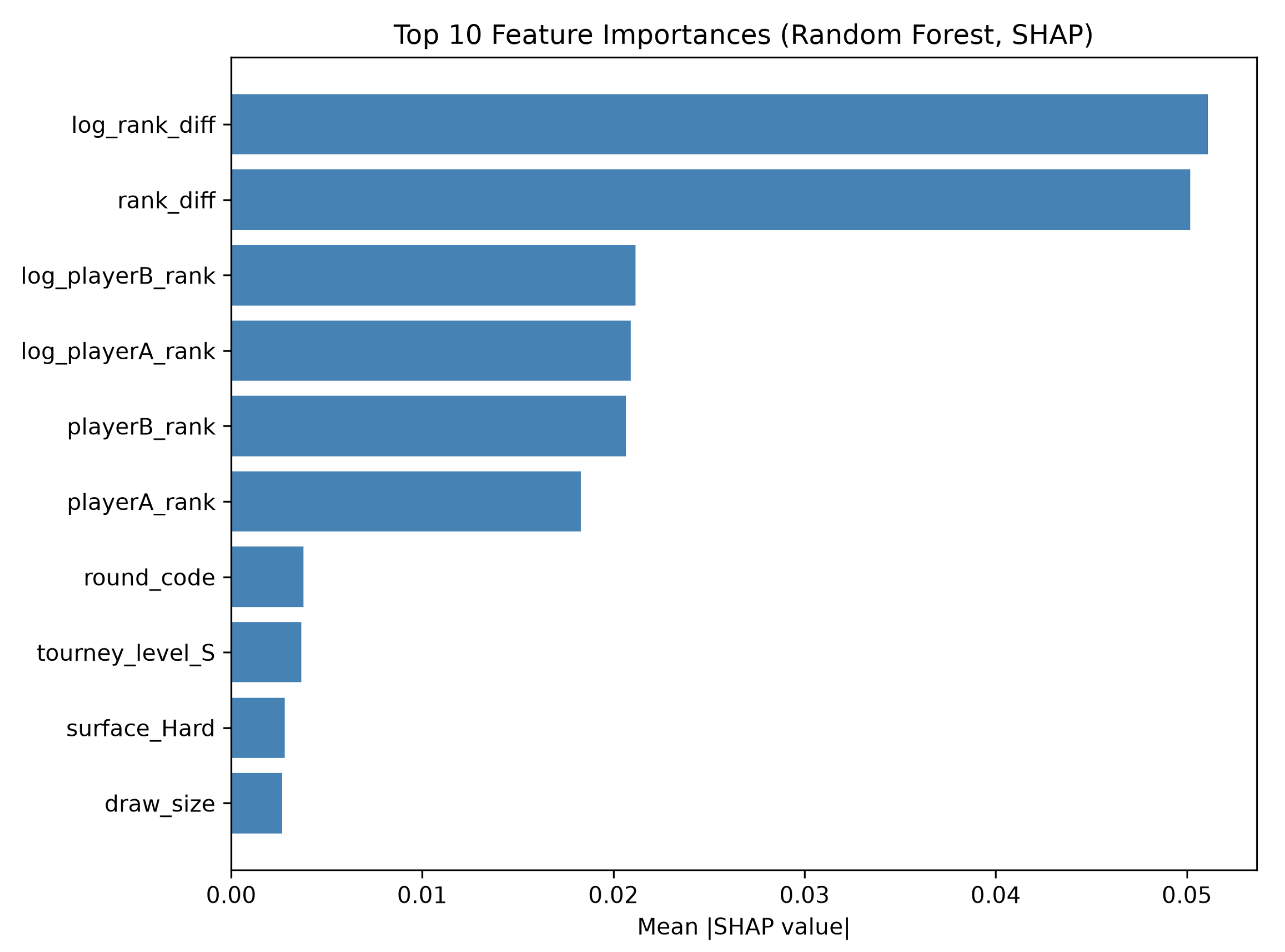
Feature importance analysis from the Random Forest model (Figure 4) was assessed using SHAP (SHapley Additive exPlanations) values computed via a TreeExplainer on 500 held-out test observations, providing a decorrelated measure of each feature’s contribution that avoids the double-counting of correlated features inherent in native Gini importance. The log-transformed rank difference and raw rank difference dominated, carrying substantially more signal than individual player ranks once correlated signal is properly attributed. Aggregating the per-feature importances into the three semantic groups defined by the input vector yields the breakdown shown in

Table 5. Feature category breakdown of Random Forest feature importance. The 16-feature input vector is partitioned into three semantic groups, and per-feature importances are aggregated within each group. Ranking features account for the bulk of predictive contribution, with surface and tournament-context features providing complementary signal.

Category	Features	Total Importance (%)
Ranking	rank_diff, log_rank_diff, player_a_rank, player_b_rank, log_player_a_rank, log_player_b_rank	77
Surface	surface_hard, surface_clay, surface_grass, surface_carpet	12
Tournament Context	tournament_level, round, best_of, draw_size, year	11

: ranking features account for 77% of total importance, surface features for 12%, and tournament-context features for the remaining 11%. Cross-validation stability was high for the top models, with standard deviations across the five folds of 0.12 pp for Histogram-Based Gradient Boosting, 0.15 pp for standard Gradient Boosting, and 0.18 pp for Random Forest.

3.4. Deep Neural Network Results

Table 6. Deep neural network configuration performance on the held-out test set (representative subset).

Configuration	Arch.	Layers	Dims	Params	Acc. (%)	ROC-AUC
Tiny-Plain	Plain	8	768	207 K	66.18	0.7247
Small-Plain	Plain	8	768	1.3 M	66.21	0.7249
Medium-Plain	Plain	12	768	9.5 M	66.19	0.7248
Large-Plain	Plain	8	768	21 M	66.17	0.7246
Tiny-Residual	Residual	8	768	207 K	66.20	0.7249
Small-Residual	Residual	8	768	1.3 M	66.22	0.7250
Medium-Residual	Residual	12	1024	9.5 M	66.20	0.7249
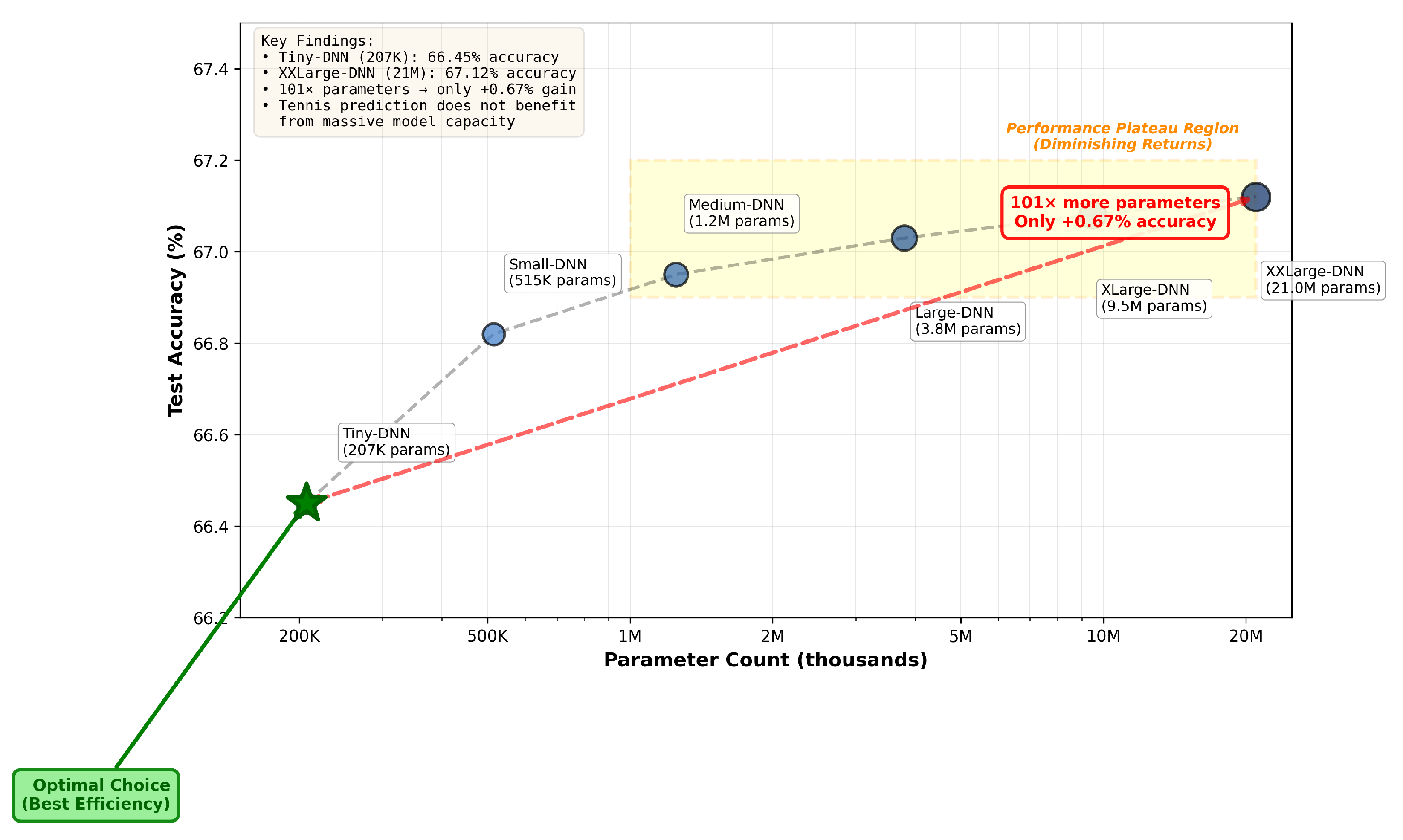
Large-Residual	Residual	8	768	21 M	66.18	0.7247

summarizes a representative subset of the 17 deep neural network configurations evaluated, spanning plain and residual architectures across the full range of model sizes. The most striking result is the absence of a meaningful effect of model size on test accuracy. The tiny model (207,000 parameters) achieved 66.18% accuracy; the large model (21,000,000 parameters, a 100-fold capacity increase) achieved 66.17%. All 17 configurations clustered within a 0.07 pp accuracy band (66.15–66.22%). The relationship is visualized across all configurations in Figure 5.

Residual connections provided marginal but consistent benefits, outperforming their plain counterparts by 0.02–0.05 pp on average. Network depth showed no consistent trend beyond a minimum functional threshold of approximately six layers, and hidden-layer dimensionality had minimal impact, with 512-, 768-, and 1024-dimensional variants all within 0.06 pp. Regularization analysis indicated that dropout rates of 0.15–0.25 and $L_2$ weight decay of ${10}^{-4}$ to $5\times {10}^{-4}$ worked best; values outside these ranges caused mild over- or under-fitting that reduced accuracy by 0.2–0.3 pp.

The best deep network—the Small-Residual configuration with eight layers, 768 hidden units, and approximately 1,300,000 parameters—achieved 66.22% accuracy and a ROC-AUC of 0.7250 on the test set.

3.5. ELO-ML Hybrid Approach Results

Augmenting the classical machine learning feature set with the three Elo-derived features produced consistent and substantial improvements across all three algorithms tested.

Table 7. Accuracy improvement from Elo feature augmentation. All improvements are statistically significant at $p<0.001$ (McNemar’s test). $\Delta$ Acc. denotes the accuracy improvement in percentage points.

Algorithm	Without Elo (%)	With Elo (%)	$\Delta$ Acc. (pp)	ROC-AUC (With Elo)	Brier (With Elo)
Logistic Regression	65.82	67.45	+1.63	0.7312	0.2067
Ridge Classifier	65.81	67.38	+1.57	0.7298	0.2074
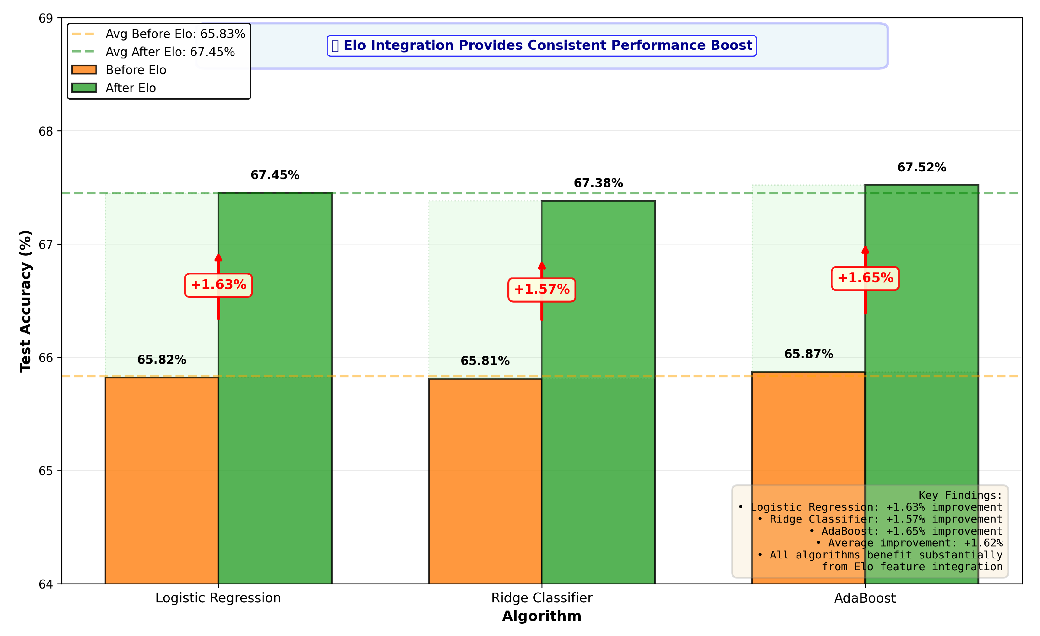
AdaBoost	65.87	67.52	+1.65	0.7305	0.2071

compares performance before and after Elo feature integration. Accuracy increased by 1.57–1.65 pp across the three algorithm families, all statistically significant at $p<0.001$ (McNemar’s test). Brier scores and ROC-AUC improved correspondingly. Computational overhead from the three additional features was negligible, with training times increasing by less than 10% relative to the standard 16-feature setup. Figure 6 visualizes the consistent accuracy uplift.

The consistency of the improvement across linear probabilistic, linear discriminative, and boosting-ensemble families indicates that the gain stems from genuine additional information content carried by Elo ratings rather than from a fortuitous interaction with any particular algorithm.

3.6. Comparative Analysis Across Approaches

3.6.1. Accuracy and Discrimination

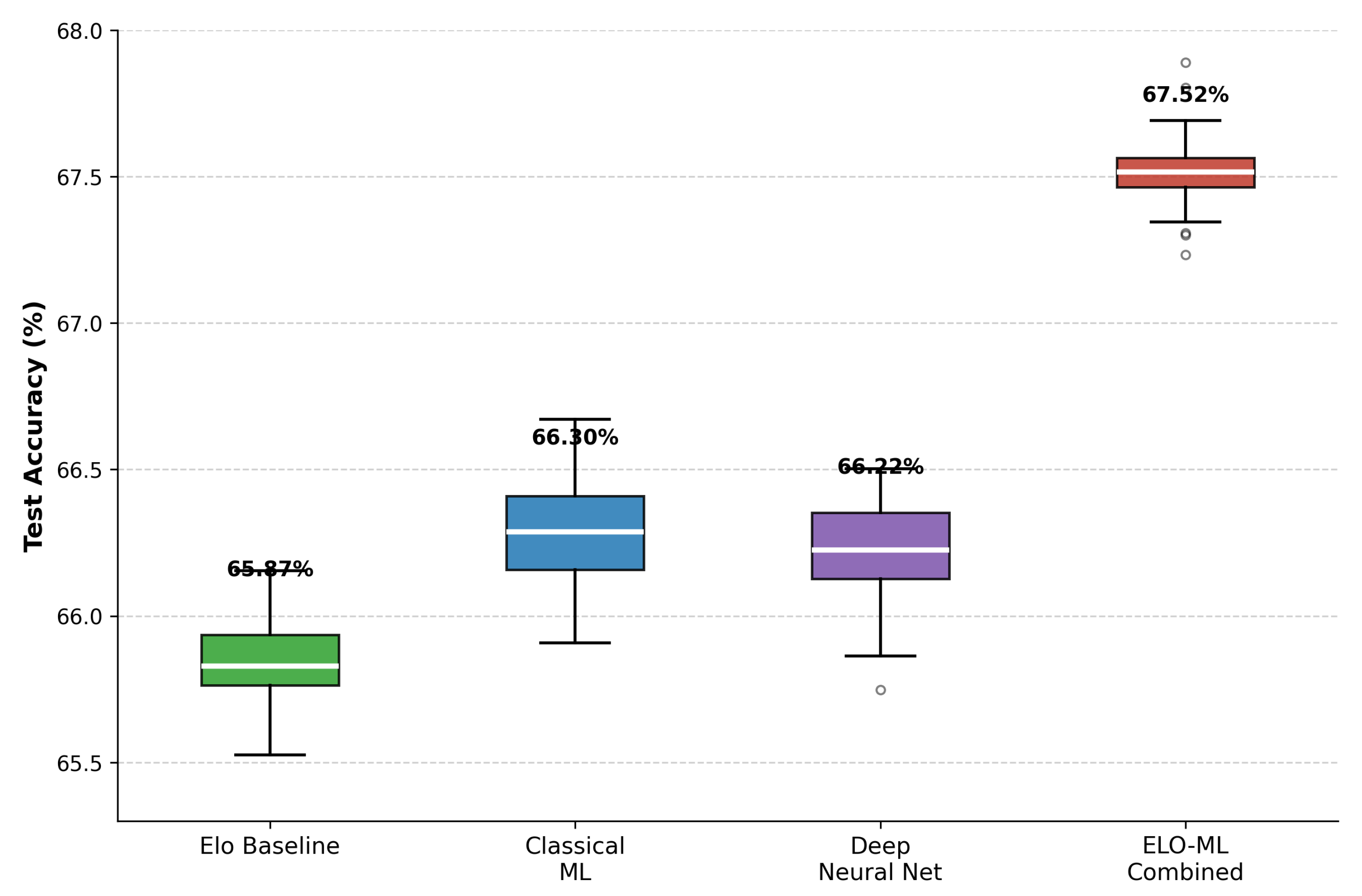
Figure 7 summarizes the head-to-head accuracy across all four approaches with 95% confidence intervals. The ELO-ML approach (67.52%) outperforms classical machine learning (66.30%), deep neural networks (66.22%), and the Elo baseline (65.87%). The 1.65 pp gap between the Elo baseline and the best ELO-ML model corresponds to a 4.8% relative reduction in error rate, a meaningful margin in a domain where most published comparisons differ by fractions of a percentage point.

Discriminative ability, measured by ROC-AUC, follows the same ranking with smaller absolute differences: 0.7305 (ELO-ML), 0.7253 (classical ML), 0.7250 (DNN), and 0.7245 (Elo). The narrower AUC range (0.0060) relative to the accuracy range (1.65 pp) indicates that the methods discriminate winners from losers at broadly similar levels; the accuracy differences arise primarily from the placement of the decision threshold relative to the predicted probability distribution.

3.6.2. Statistical Significance

McNemar’s test was applied to all pairwise comparisons among the top models, with results reported in

Table 8. Statistical significance of pairwise accuracy differences via McNemar’s test on the held-out test set (n = 86,691). Differences are reported in percentage points (pp).

Model 1	Model 2	Acc. Diff. (pp)	p-Value
ELO-ML AdaBoost (67.52%)	Classical ML HGB (66.30%)	+1.22	<$0.001$
ELO-ML AdaBoost (67.52%)	DNN Small-Residual (66.22%)	+1.30	<$0.001$
ELO-ML AdaBoost (67.52%)	Elo Baseline (65.87%)	+1.65	<$0.001$
Classical ML HGB (66.30%)	DNN Small-Residual (66.22%)	+0.08	0.31
Classical ML HGB (66.30%)	Elo Baseline (65.87%)	+0.43	<$0.001$
DNN Small-Residual (66.22%)	Elo Baseline (65.87%)	+0.35	<$0.001$
ELO-ML Logistic (67.45%)	ELO-ML AdaBoost (67.52%)	$-0.07$	0.18

. The ELO-ML AdaBoost model significantly outperformed every other approach at $p<0.001$, with the smallest margin (1.22 pp over classical machine learning) still corresponding to a statistically reliable difference given the test-set size of 86,691 observations. The 0.08 pp difference between the best classical machine learning model and the best deep neural network was not significant ($p=0.31$), providing direct empirical evidence that the two paradigms achieve equivalent accuracy for this task. Both, in turn, significantly outperformed the Elo baseline ($p<0.001$), confirming that machine learning extracts genuine additional signal beyond what Elo ratings capture. The 0.07 pp gap between ELO-ML Logistic Regression and ELO-ML AdaBoost was not significant ($p=0.18$), indicating that both are viable deployment choices.

3.6.3. Calibration Quality

Although classical and deep models are statistically indistinguishable in accuracy, they differ substantially in probability calibration.

Table 9. Calibration metrics for the best model from each approach on the held-out test set.

Model	ECE	Brier Score	Log Loss
DNN (Small-Residual)	0.0077	0.2098	0.6187
ELO-ML Combined (AdaBoost)	0.0089	0.2071	0.6154
Classical ML (Hist. Gradient Boosting)	0.0142	0.2101	0.6192
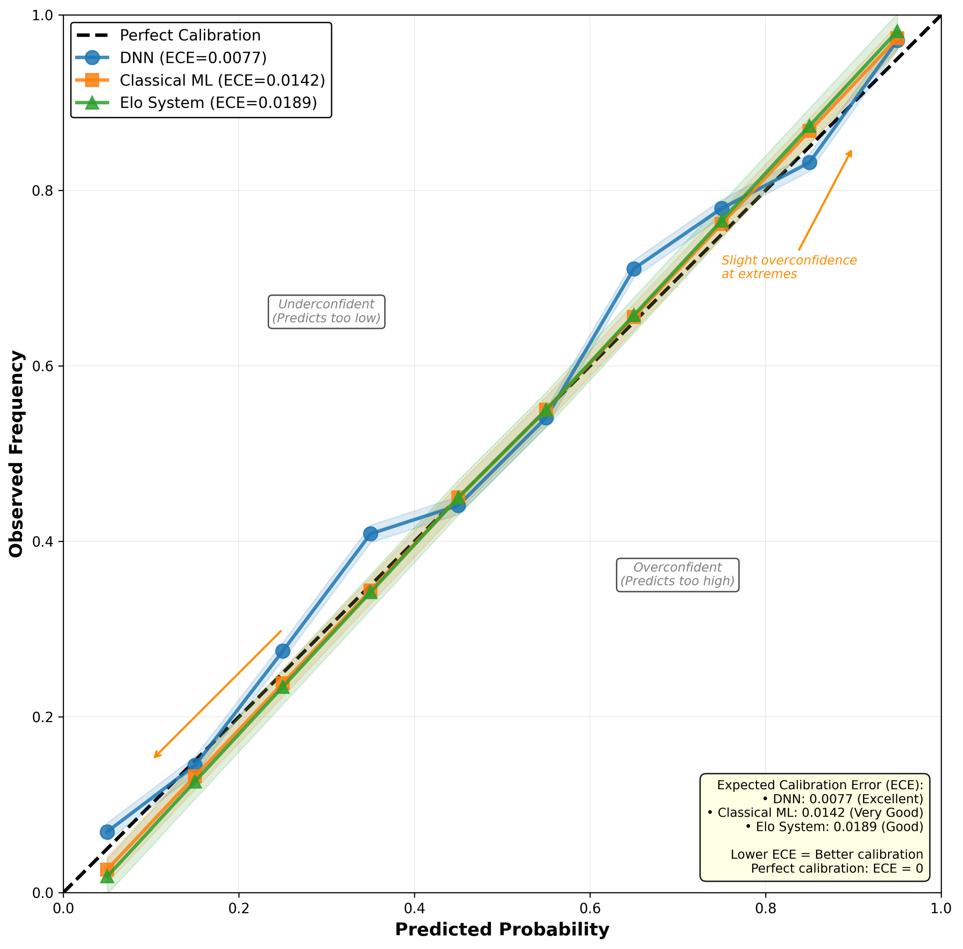
Elo Rating System	0.0189	0.2120	0.6234

summarizes the calibration metrics for the best model from each approach. The best deep neural network achieved the lowest ECE at 0.0077, nearly half that of the best classical model (0.0142) and considerably better than the Elo baseline (0.0189). The ELO-ML approach was close behind in ECE (0.0089), and notably achieved both the lowest Brier score (0.2071) and the lowest log loss among the approaches—reflecting that its overall probability estimates are closest to the true outcome probabilities in mean squared error, even though bin-level calibration is marginally tighter for the DNN. Figure 8 shows reliability diagrams for the three best models.

The deep network’s superior bin-level calibration stems plausibly from architectural and training choices: a sigmoid output combined with the binary cross-entropy loss directly optimizes probability quality, penalizing confident incorrect predictions, whereas tree-based ensembles aggregate discrete leaf-level votes and can therefore produce systematically miscalibrated probabilities even when classification accuracy is high.

3.6.4. Computational Efficiency

Table 10. Computational requirements for the best model from each approach.

Approach	Training Time	Prediction Time	Memory (MB)
Elo Rating System	— (online)	∼0.1 s	8
ELO-ML Logistic Regression	23 s	1.3 s	18
ELO-ML AdaBoost (Best Acc.)	87 s	3.4 s	142
Classical ML Hist. Gradient Boosting	68 s	2.9 s	89
DNN Tiny (207 K params)	130 s	2.1 s	23
DNN Large (21 M params)	7200 s	8.4 s	418

summarizes the computational requirements of the best model from each approach, expressed as training time, prediction time, and peak memory usage. The Elo baseline requires no supervised training and produces near-instantaneous predictions; among the supervised approaches, ELO-ML Logistic Regression provides the most favorable accuracy-to-efficiency trade-off, reaching 67.45% accuracy (only 0.07 pp below the best model) while training in 23 s with an 18 MB memory footprint. The best supervised model overall—ELO-ML AdaBoost at 67.52%—trains in 87 s with 142 MB. At the other extreme, the largest deep neural networks require GPU resources for over 7200 s of training time with 418 MB of memory while delivering no accuracy advantage over the 207,000-parameter tiny network.

4. Discussion

4.1. Interpretation of the Performance Hierarchy

The strongest single finding of this study is how narrow the headroom above Elo actually is on this task. A well-tuned Elo baseline alone reaches 65.87% test accuracy with no machine learning, and the best of ten classical ML algorithms, seventeen deep neural network configurations, and the hybrid ELO-ML approach—together representing dozens of distinct models, hundreds of hyperparameter configurations, and a 100-fold range in parameter count—add only between 0.43 pp and 1.65 pp on top of that baseline. All four approaches sit within a 1.65 pp band whose upper edge (67.52%) remains meaningfully below the 70–72% accuracy band that Kovalchik [1] documents for bookmaker odds, which incorporate information unavailable to any statistical model trained on standard pre-match features. The dominant signal here is therefore not the ranking of methods but the floor and ceiling of the task: Elo alone captures most of what can be captured from universally available pre-match features, and even the best learned model in the comparison remains below market-implied accuracy.

This narrow band is consistent with the structural character of professional men’s tennis as a small-margin sport. In elite Grand Slam matches the server wins approximately 63–65% of points across surfaces—meaning that even at the highest level the receiver wins only roughly one point in three—so most games are held and match outcomes are decided by a small minority of points in which serve is broken [31]. Because the scoring system is non-linear, the player who wins fewer total points can still win the match: Lisi et al. [32] report that 4.18–4.78% of ATP matches in the 2000s and 2010s were won by the player with strictly fewer total points. Single-match instances illustrate the effect more sharply. In the 2019 Wimbledon men’s final Djokovic defeated Federer despite winning 204 of the 422 total points to Federer’s 218—losing the volume statistics in nearly every category—and prevailed by saving two championship points and converting all the tiebreaks [33]. More recently, in the 2026 Australian Open semifinal Djokovic defeated Sinner 3–6, 6–3, 4–6, 6–4, 6–4 after saving 16 of the 18 break points he faced, including all 8 in the deciding set, despite trailing on most volume metrics for much of the match [34]. In a sport where outcomes can hinge on a handful of correctly-played critical points and substantial within-match noise is structurally absorbed by the scoring system, much of the variance in match outcomes is by construction not captured by static, pre-match summary features. A 65–67% pre-match-feature accuracy ceiling, with all four model classes clustered near it, is therefore in large part a property of the sport rather than a property of any particular learner.

Within this narrow band, the ELO-ML hybrid is the strongest model, achieving a consistent +1.57–1.65 pp uplift across three algorithm families—linear probabilistic, linear discriminative, and boosting-ensemble—all statistically significant at $p<0.001$ by McNemar’s test on n = 86,691 held-out matches. The cross-family consistency rules out the hypothesis that the uplift is an artifact of a fortuitous interaction with any specific learner and provides empirical evidence on tour-level data for the SEL framework [18], extending the Grand-Slam-only results of Buhamra et al. [19] to general tour-level competition. Mechanistically, the improvement is interpretable: Elo ratings encode three pieces of information that ATP rankings do not capture explicitly—recent form (through continuous updating after every match), strength of schedule (through the magnitude of updates given opponent quality), and surface specialization (through independent per-surface ratings)—which are predictive of match outcomes but absent from the standard 16-feature input. We emphasize, however, that the absolute size of the uplift is modest. At roughly an order of magnitude above the 0.12–0.18 pp five-fold cross-validation standard deviation of the top classical models, and small relative to the 70–72% bookmaker-accuracy band that remains out of reach for all four approaches, the gain is best read as a useful but marginal augmentation rather than a state-of-the-art breakthrough.

The statistically indistinguishable accuracy of the best classical machine learning model (66.30%) and the best deep neural network (66.22%, $p=0.31$) challenges the increasingly common assumption that deep learning offers a default accuracy advantage on any sufficiently complex task. For structured tabular sports data of moderate size, the experimental evidence here is clear: properly tuned ensemble learners match deep networks on accuracy. This is consistent with broader recent findings in tabular machine learning, where deep methods often fail to outperform gradient-boosted trees absent task-specific architectural innovations or much larger datasets [12,13].

Yet the two paradigms are not interchangeable. Deep neural networks achieve substantially better probability calibration (ECE 0.0077 vs. 0.0142, a 46% reduction), a distinction that matters wherever predicted probabilities themselves are used—in risk assessment, in Kelly-criterion bet sizing, or in any decision-support application where overconfident incorrect predictions are particularly costly. Practitioners therefore face a meaningful trade-off: classical ensemble methods offer lower training cost, simpler deployment, and direct interpretability via feature importance; deep networks offer better-calibrated probabilities at the cost of more elaborate infrastructure.

The most actionable architectural finding is the absence of any benefit from scale. All 17 deep network configurations cluster within a 0.07 pp accuracy band despite a 100-fold variation in parameter count. Increasing capacity from 207,000 to 21,000,000 parameters yields zero measurable improvement on this task. The most parsimonious explanation is that, given the 16-feature input vector and the approximately 400,000 training observations, the task carries only a limited amount of learnable signal, which even a tiny network captures fully. Once that signal is captured, additional capacity is redundant. This stands in marked contrast to the well-known scaling behavior of computer vision and language models [35] and provides empirical grounding for a clear deployment recommendation: in structured-tabular sports prediction, deploy the smallest network that reaches the performance plateau.

4.2. Comparison with Prior Work

The 67.52% best accuracy reported here lies within the band most commonly observed in the literature for general tour-level pre-match tennis prediction. Kovalchik [1] described a long-standing 70–72% upper bound for sophisticated Elo-style models on this task, with no statistical model consistently outperforming bookmaker odds; the present results sit slightly below that bound. Higher accuracies of 80% and above reported by some studies—most notably Gao and Kowalczyk [10], who used Random Forests with detailed serve and return statistics, and Li et al. [36], who reported very high accuracies for mid-match predictions with in-play data—rely on richer or in-play feature sets unavailable for pre-match prediction across a multi-decade tour-wide dataset. The strong convergence between the present results and Wilkens [13], who observed an approximate 70% ceiling across multiple algorithm families on standard features, reinforces the conclusion that the dominant ceiling on pre-match prediction accuracy is set by feature richness, not by algorithmic sophistication.

Several deep learning studies have reported gains over classical baselines on tennis. Candila and Palazzo [3] demonstrated that feed-forward neural networks with a rich feature set could outperform several traditional baselines, though their advantage over a carefully specified Logistic Regression was modest. Jiang and Yuan [11] found LSTM models effective for in-match momentum prediction but offering no advantage for pre-match settings. The present study aligns with the strand of literature that finds deep models competitive but not superior on pre-match accuracy, while extending it by quantifying the architecture-scaling relationship across 17 configurations and demonstrating the equivalence under McNemar’s significance testing.

The empirical support found here for the SEL framework [18] is consistent with, and substantially extends, the work of Buhamra et al. [19], who reported improvements from Elo features in Grand Slam prediction. By demonstrating that the gain is essentially constant across three algorithm families and on data spanning the full tour, the present results address the principal open question left by their study—whether the SEL benefit generalizes beyond a single algorithm and beyond Grand Slam matches.

4.3. Practical Implications

The findings translate into concrete deployment guidance for sports analytics practitioners.

Prefer feature engineering over architectural complexity. The 1.65 pp improvement from a three-feature Elo augmentation exceeds anything achieved by 100-fold increases in deep network capacity. In limited-data tabular domains with established statistical models, the highest-return investment is typically in data enrichment and domain-informed feature engineering rather than in scaling models.

Match model choice to deployment constraints. For pure accuracy on this task, ELO-ML AdaBoost is the strongest model. For the best efficiency-to-accuracy trade-off, ELO-ML Logistic Regression—at 67.45% accuracy, 23 s training time, and 18 MB memory—is essentially interchangeable with the best model on accuracy ($p=0.18$) while running comfortably on commodity hardware. For applications where calibrated probabilities are central, deep networks deliver substantially better ECE at modest additional cost; a 207,000-parameter tiny network is sufficient.

Avoid over-parameterized deep models.Large neural networks offer no accuracy benefit for this task. The 21,000,000-parameter network requires 55× longer training and 18× more memory than the 207,000-parameter variant for an accuracy difference of 0.01 pp, with the smaller network actually outperforming on some metrics. Deployment on resource-constrained edge devices is therefore practical without any accuracy sacrifice.

For applications in regulated sports betting markets, the implications are more nuanced. The 67.52% best accuracy remains below the 70–75% accuracy commonly cited for bookmaker odds [1], which incorporate information unavailable to statistical models (late-breaking injury news, market sentiment, expert judgment). A direct profitability comparison against historical betting markets was outside the scope of this study and would require dedicated evaluation against opening and closing lines, transaction costs, and Kelly-criterion bet sizing. The superior calibration of the ELO-ML and DNN models, however, suggests that they would be better suited than pure Elo for any probability-dependent decision rule.

4.4. Limitations

Several limitations of this study should be acknowledged. First, on the data side, the standardized 16-feature input deliberately excludes serve and return statistics, point-by-point telemetry, and player fitness or injury data, which prior work has shown can substantially improve accuracy when available [10,36]. The reliance on universally available features ensures comparability across the 1968–2024 span at the cost of an upper bound on achievable accuracy. Second, the analysis is restricted to the men’s ATP tour; whether the findings generalize to the women’s WTA tour, to doubles, or to lower-tier competitions remains an empirical question. Third, the deep learning architecture sweep, while spanning a 100-fold range of capacity, is confined to MLPs; tabular Transformers (e.g., TabTransformer, FT-Transformer), TabNet, and graph neural networks were not evaluated. Given the sharp plateau observed across MLP capacity, however, breakthroughs from architectural innovation alone—without accompanying data enrichment—appear unlikely. Fourth, no direct evaluation against historical bookmaker odds was performed, so claims about economic utility remain qualitative. Finally, model interpretability was assessed via SHAP values on the Random Forest model; future work could extend this analysis to other model families using LIME or integrated gradients.

4.5. Future Work

Several directions follow naturally from these limitations. The highest-return extension is data enrichment: incorporating point-by-point match data, player fitness and travel data, head-to-head detail beyond simple counts, and—where appropriate—textual information from match reports and player interviews. On the modeling side, advanced tabular architectures (TabTransformer, FT-Transformer, TabNet) should be tested directly against the benchmarks established here, particularly in combination with SEL-style feature augmentation. Stacked ensembles that combine the complementary strengths of gradient boosting (sharp decision boundaries), deep networks (well-calibrated probabilities), and ELO-ML (domain knowledge integration) merit dedicated study and could plausibly push accuracy into the 68–69% range. Online learning systems that update model parameters as new matches arrive would address the static-model limitation of the current study and could absorb gradual drift in playing styles, surface speed, and competitive balance. Subgroup analyses—by surface, tournament tier, ranking range, and match competitiveness—would identify the contexts in which models are reliable and those in which additional caution is warranted. Finally, extending the framework to the WTA tour and to other sports would test the cross-domain generalizability of the headline findings reported here.

5. Conclusions

We have presented a unified empirical comparison of four distinct paradigms for professional tennis match prediction—an enhanced Elo rating system, ten classical machine learning algorithms, seventeen deep neural network configurations, and a hybrid ELO-ML approach—evaluated on the same 133,138-match dataset with identical temporal train–validation–test splits and a common suite of metrics. The unified design eliminates the dataset, feature, and protocol confounds that complicate cross-study comparison in the existing literature.

Four headline findings emerge. First, pre-match tennis prediction under universally available features is a fundamentally difficult task with a low ceiling: a tuned Elo baseline alone reaches 65.87% accuracy, all four approaches studied here sit within a 1.65 pp band (65.87–67.52%), and even the best model in the comparison remains below the 70–72% accuracy commonly cited for bookmaker odds. The dominant constraint on accuracy is feature richness, not algorithmic sophistication. Second, deep network capacity exhibits sharply diminishing returns: 17 configurations spanning a 100-fold range of parameter count cluster within a 0.07 pp accuracy band, indicating that the prediction task is constrained by data richness and feature dimensionality rather than by model expressiveness; classical machine learning and deep neural networks are themselves statistically indistinguishable in accuracy ($p=0.31$, 0.08 pp gap), although deep networks deliver substantially better probability calibration (ECE 0.0077 vs. 0.0142). Third, augmenting classical learners with three Elo-derived features yields a consistent +1.57–1.65 pp uplift across three algorithm families ($p<0.001$ by McNemar’s test), with the best ELO-ML model reaching 67.52% accuracy; the cross-family consistency provides empirical evidence on tour-level data for the Statistically Enhanced Learning framework, although the absolute size of the uplift is modest and is best read as a useful augmentation rather than a categorical performance breakthrough. Fourth, deployment-efficient models are competitive: ELO-ML Logistic Regression reaches 67.45% accuracy in 23 s of training time with 18 MB of memory, statistically indistinguishable from the best model in the study.

For practitioners, the implications are clear. In structured tabular sports prediction with established domain-informed statistical models, the highest-return modeling investment is feature engineering grounded in domain knowledge—not increased model capacity. Model selection should be driven by application requirements: classical ensembles for pure accuracy with simple deployment, deep networks where well-calibrated probabilities matter, and ELO-ML hybrids when both are required. For sports analytics research, the unified evaluation framework established here provides a reproducible benchmark on which subsequent methodological innovations can be compared.