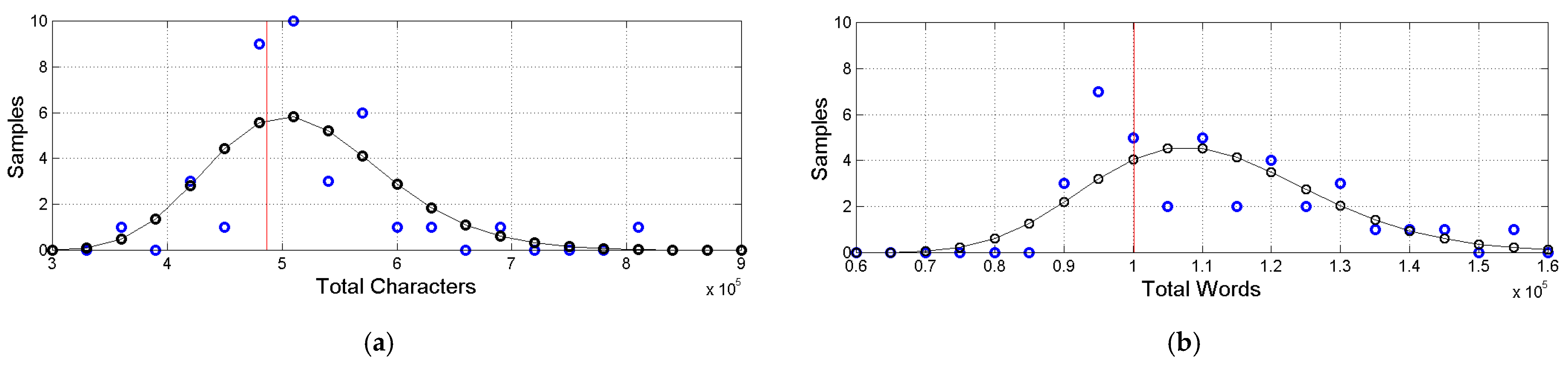
Figure 1.
(a) Histograms of total number of characters (blue circles) with the estimated log–normal model (black circles and black line). The red vertical line indicates the Greek value in abscissa. (b) Histograms of total number of words (blue circles) with the estimated log–normal model (black circles and black line). The red vertical line indicates the Greek value in abscissa.
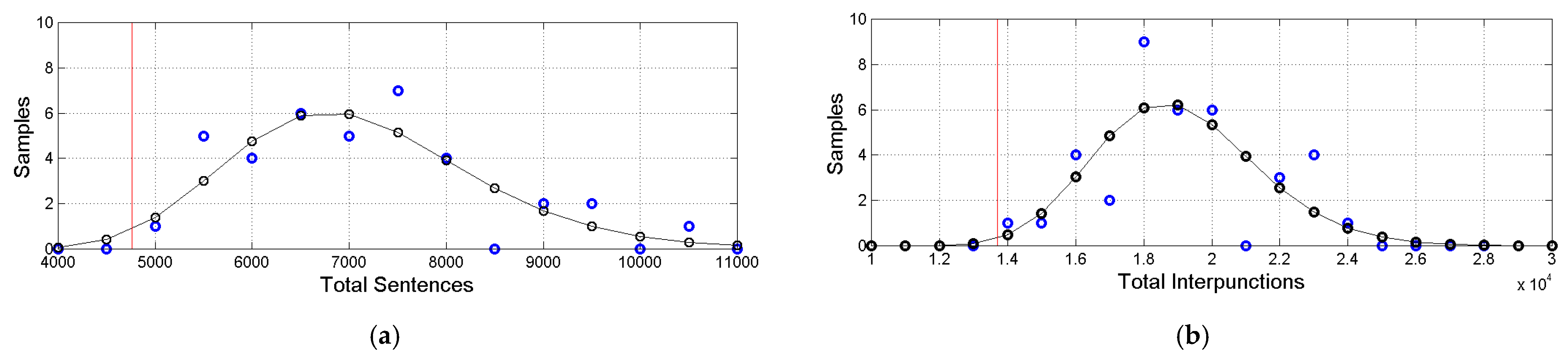
Figure 2.
(a) Histograms of total number of sentences (blue circles) with the estimated log–normal model (black circles and black line). The red vertical line indicates the Greek value in abscissa. (b) Histograms of total number of interpunctions (blue circles) with the estimated log–normal model (black circles and black line). The red vertical line indicates the Greek value in abscissa.
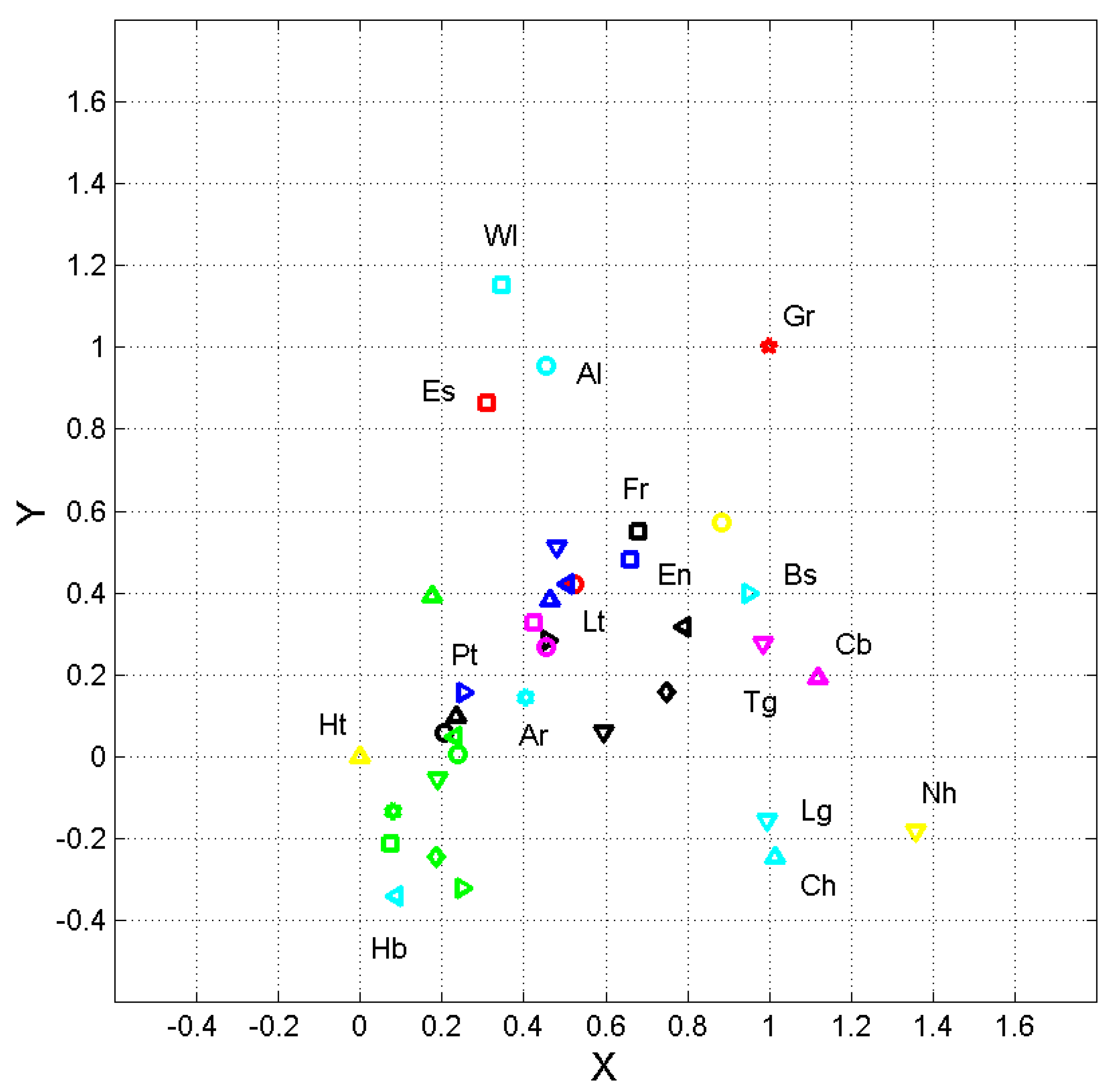
Figure 3.
Normalized coordinates and of the ending point of vector Equation (6), calculated by setting Haitian at the origin and Greek at , according to the linear transformation Equations (7) and (8). Greek, Gr; Latin, Lt; Esperanto, Es. Romance languages, blue symbols, key: French, square; Italian, triangle <; Portuguese >, Romanian, ^, Spanish, v. German languages, black symbols, key: Danish, circle; English, square; Finnish, triangle <; German, >; Icelandic, ^; Norwegian, v; Swedish, diamond. Balto–Slavic languages, green symbols, key: Bulgarian, circles; Czech, square; Croatian, <; Polish, >; Russian, ^; Serbian, v; Slovak, diamond; Ukrainian, hexagram. Uralic languages, magenta symbols, key: Estonian, circle; Hungarian, square. Albanian languages, Albanian, cyan circle. Armenian languages, Armenian, cyan hexagram. Celtic languages, Welsh, cyan square. Isolate languages, Basque, cyan triangle >. Semitic languages, Hebrew, cyan <. Austronesian languages, magenta symbols, key: Cebuano, triangle ^; Tagalog, v. Niger–Congo languages, cyan symbols; Chichewa, triangle ^; Luganda, v. Afro–Asiatic languages, Somali, yellow circle. French Creole languages, Haitian, yellow triangle ^. Uto–Aztecan, Nahuatl, yellow triangle v. Some languages are explicitly labelled because they share the same key color as other languages.
![Analytics 04 00017 g003]()
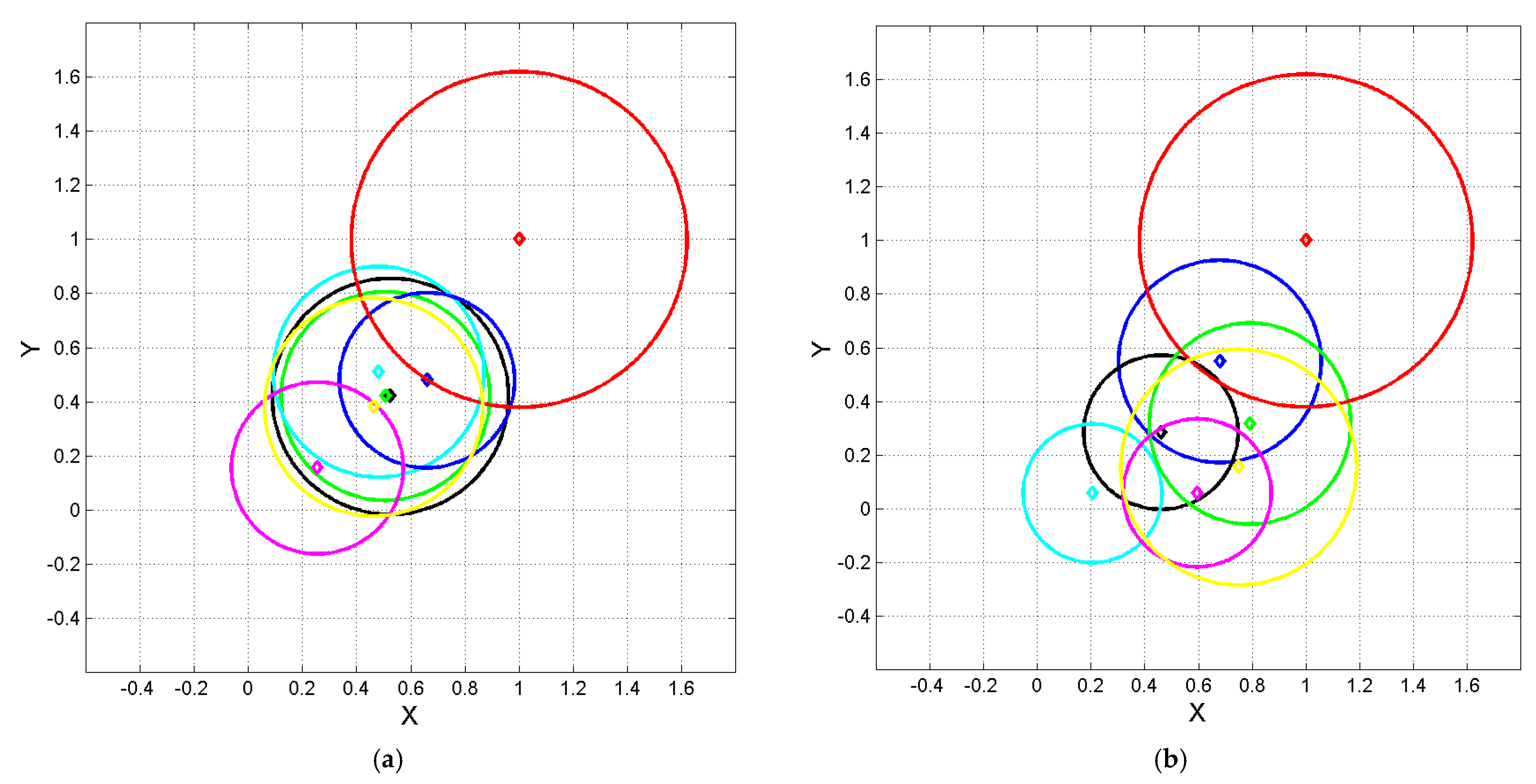
Figure 4.
Normalized coordinates and of the ending point of vector of Equation (6), calculated by setting Haitian at the origin and Greek at , according to the linear transformations (7) and (8). Diamond represents Equation (6); circles with the same color represent 1–sigma contour lines. (a) Color key: Gr red; Lt black; It green; Sp cyan; Fr blue; Pt magenta; Rm yellow. (b) Color key: Gr red; Ge black; Fn green; Dn cyan; En blue; Nr magenta; Sw yellow.
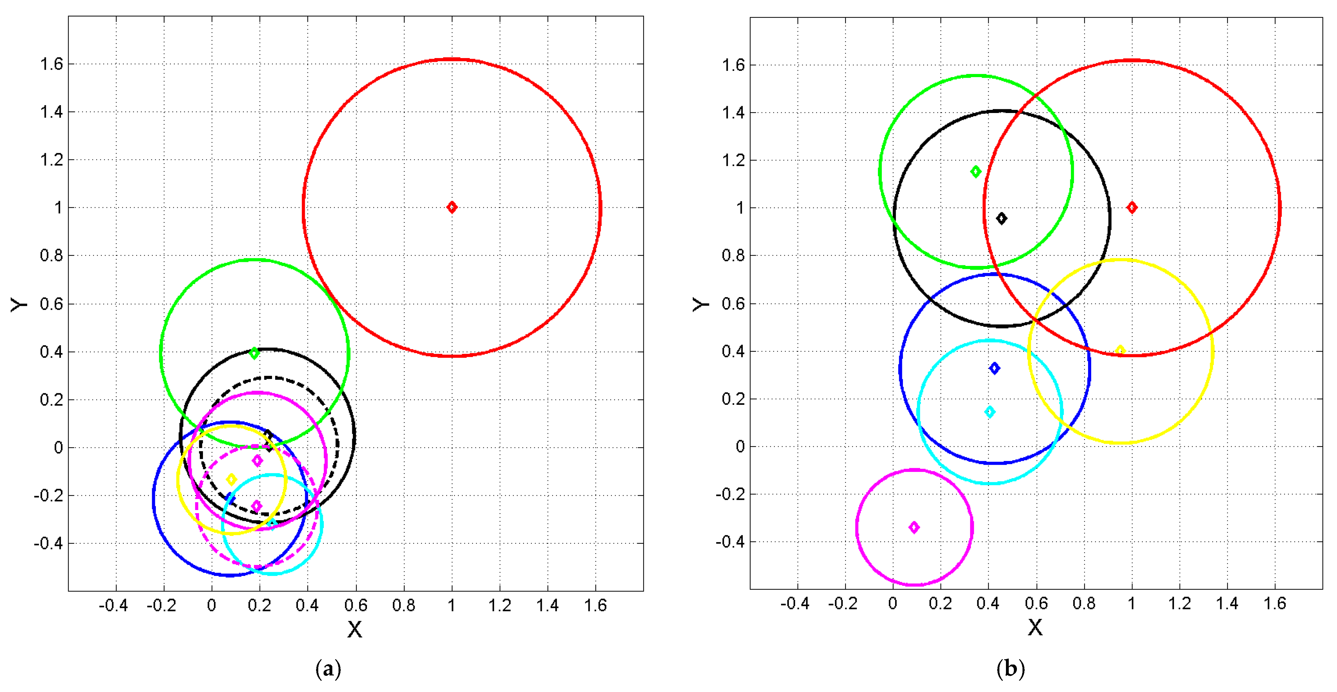
Figure 5.
Normalized coordinates and of the ending point of vector of Equation (6), calculated by setting Haitian at the origin and Greek at , according to the linear tranformations (7) and (8). Diamond represents Equation (6); circles with the same color represent 1–sigma contour lines. (a) Color key: Gr red; Bg black dashed; Cz blue; Cr black; Pl cyan; Rs green; Sr magenta; Sl magenta dashed; Uk yellow. (b) Color key: Gr red; Al black; Wl green; Ar cyan; Hn blue; Hb magenta; Bs yellow.
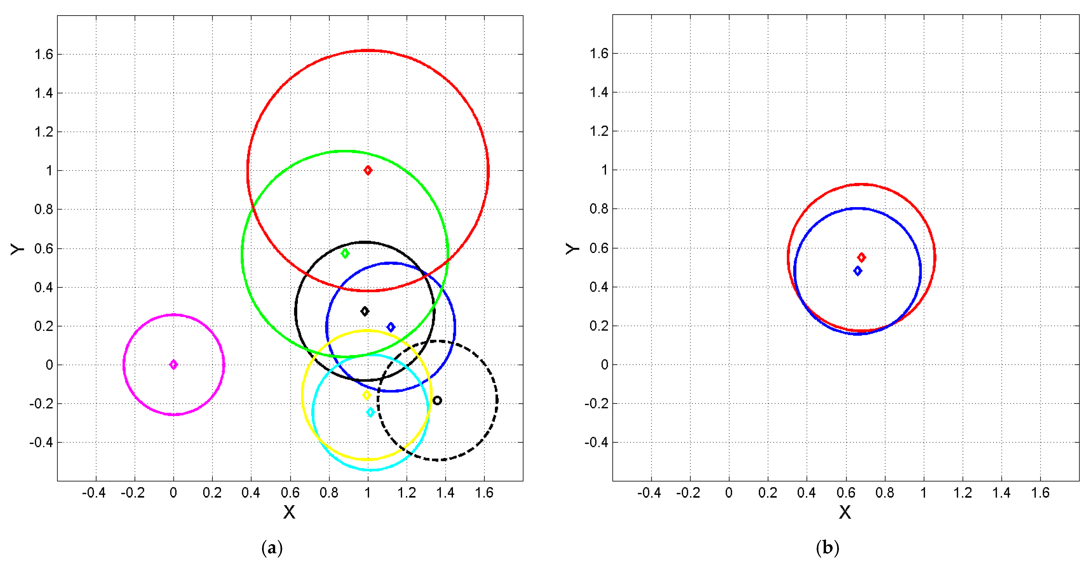
Figure 6.
Normalized coordinates and of the ending point of vector of Equation (6), calculated by setting Haitian at the origin , magenta diamond, and Greek at , red diamond, according to the linear transformations (7) and (8). Circles with the same color represent 1–sigma contour lines. (a) Color key: black Tg; green Sm; cyan Ch; blue Cb; magenta Ht; yellow Lg; black dashed Nh. (b) Color key: English red; French blue.
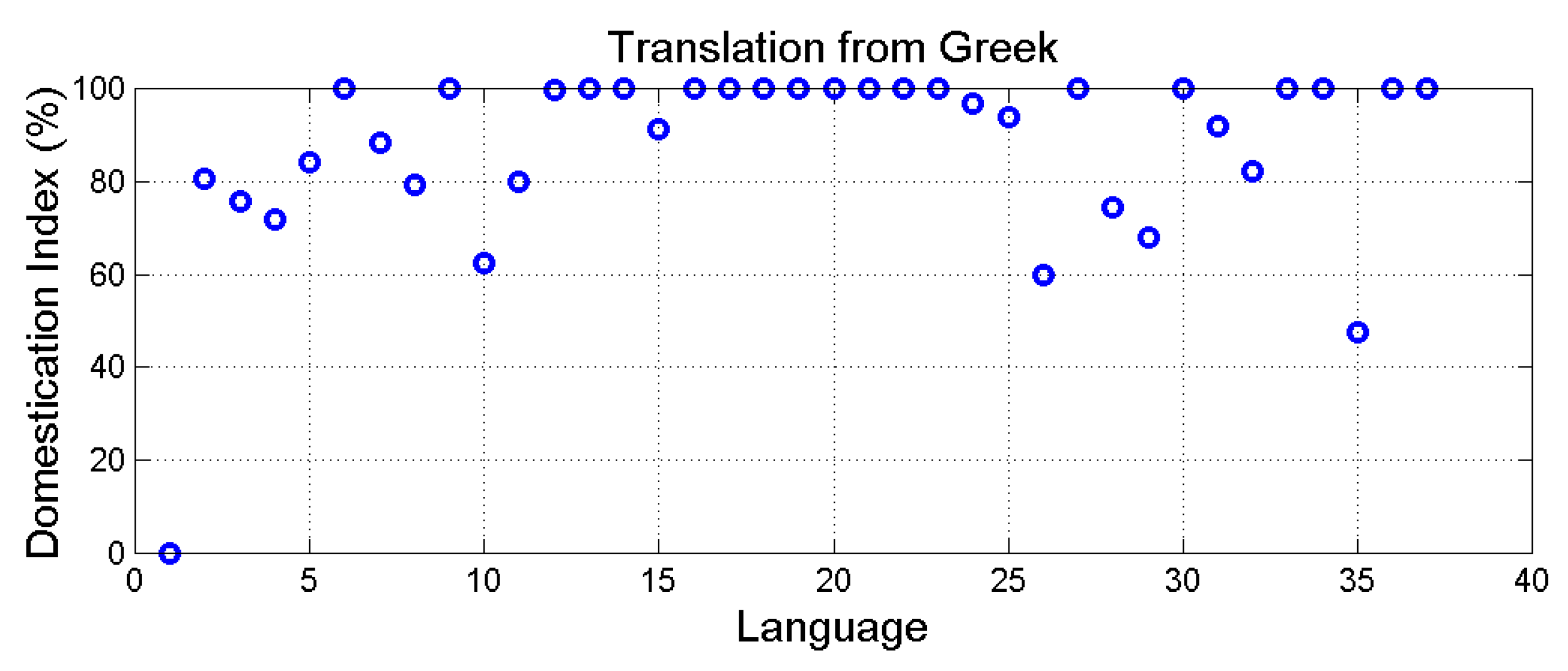
Figure 7.
Domestication index,
(%), versus translation language order (see
Table 1).
Figure 7.
Domestication index,
(%), versus translation language order (see
Table 1).
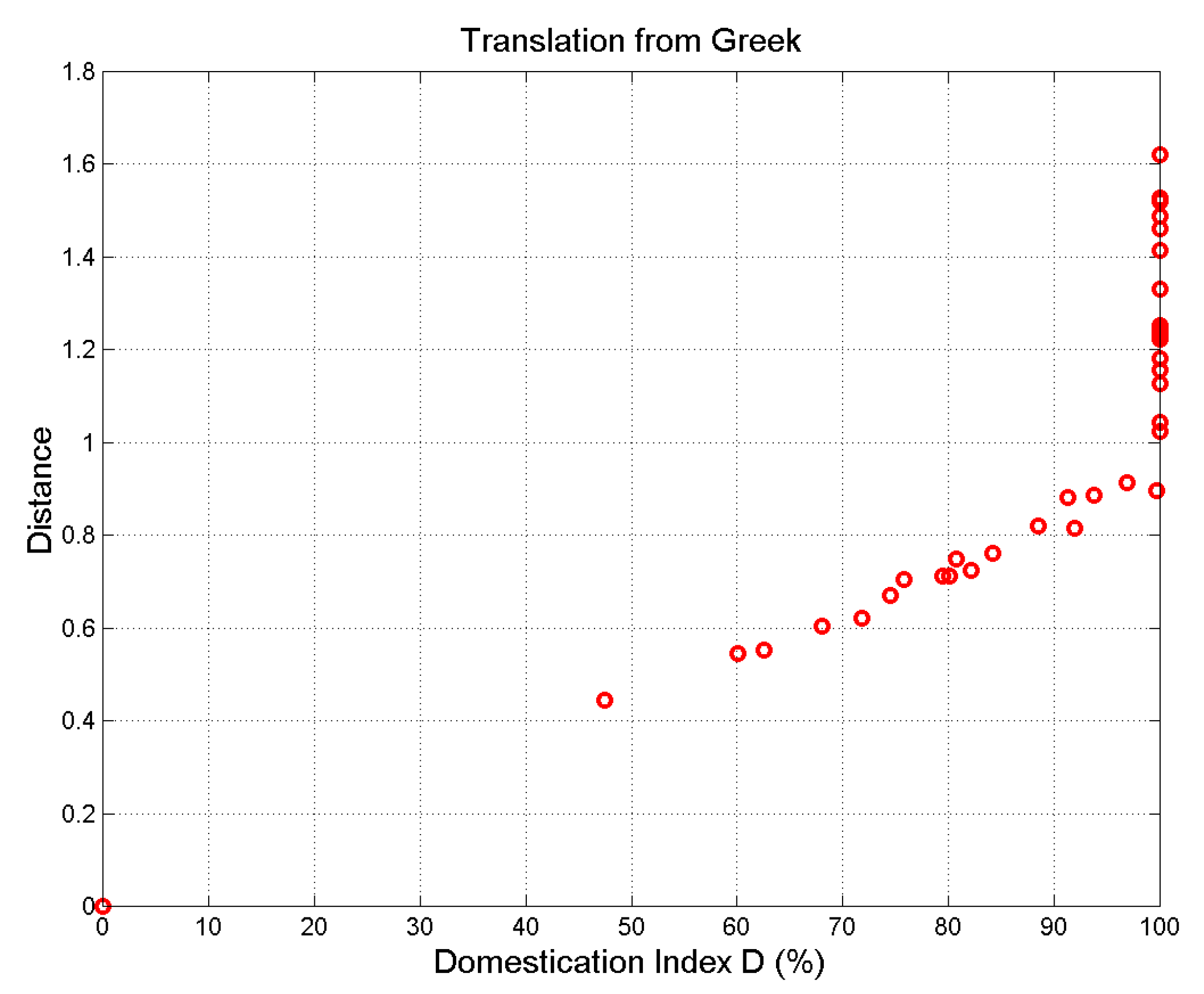
Figure 8.
Distance versus domestication index, (%), of translations from Greek. The origin corresponds to Greek.
Figure 8.
Distance versus domestication index, (%), of translations from Greek. The origin corresponds to Greek.
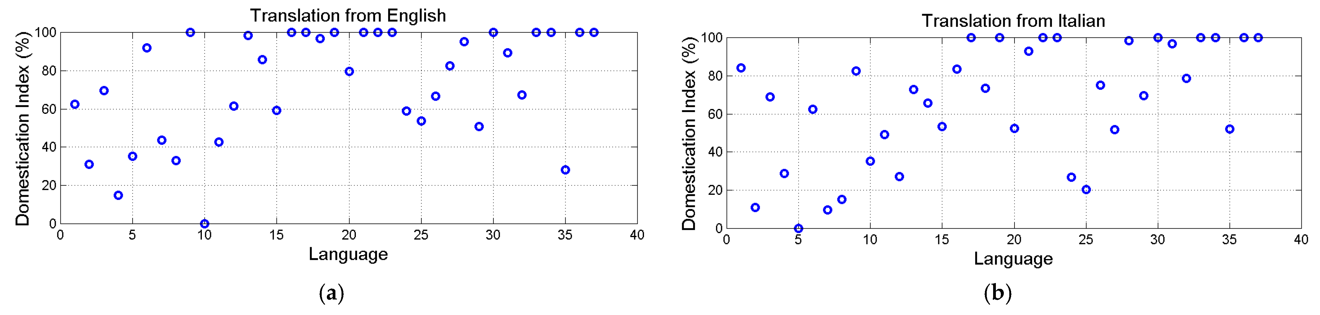
Figure 9.
Domestication index,
(%), of the alleged translation: (
a) from English to other languages (for language order number see
Table 1). English is language 10. The minimum
is found in French (language 4). (
b) From Italian to other languages. Italian is language 5. The minimum
is found in Romanian (language 7); Latin (language 2) is very close to Italian,
.
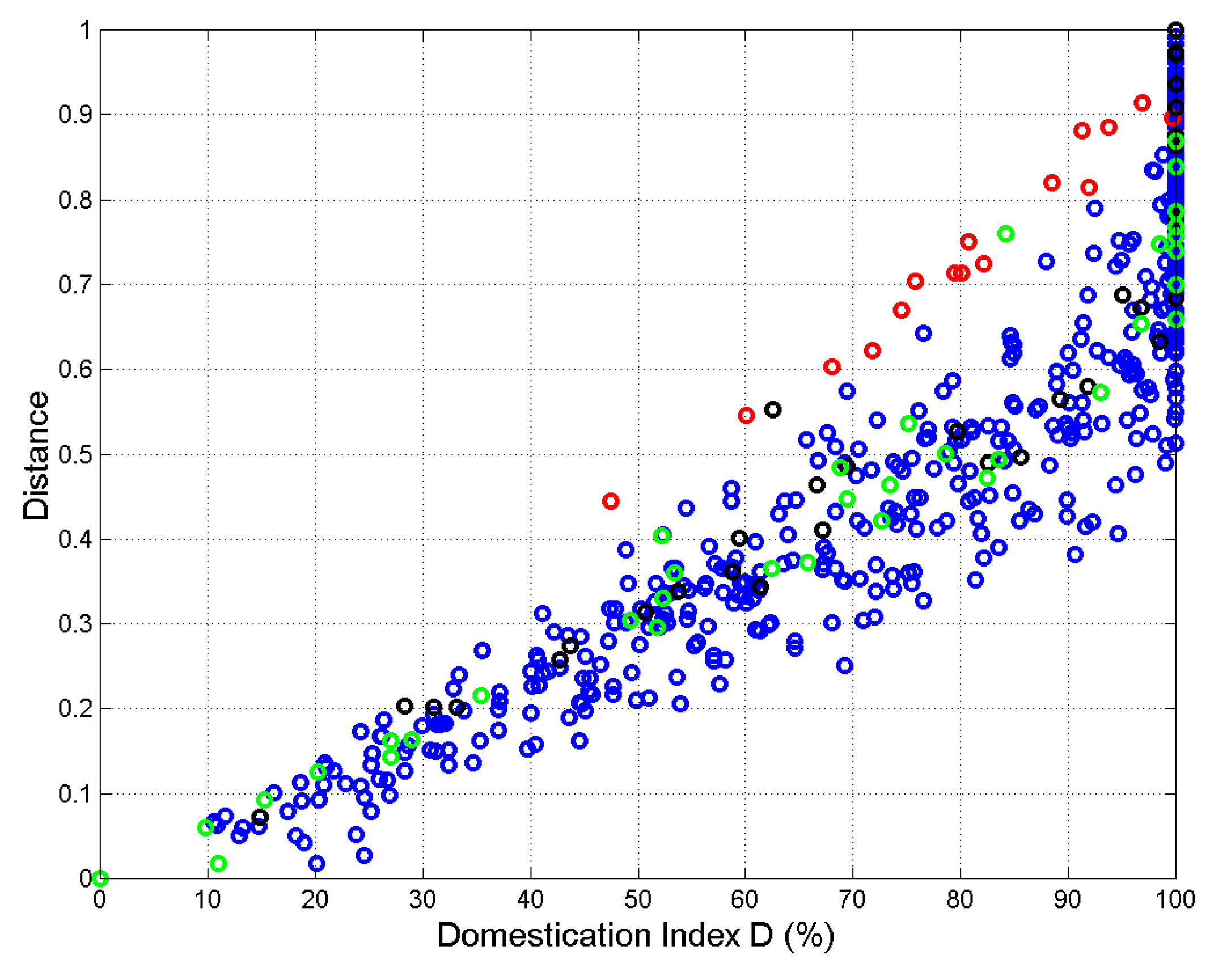
Figure 10.
Distance versus domestication index, (%). The origin corresponds to the language assumed to be the source text. Red circles refer to Greek as source texts; black circles to English, green circles to Italian, and blue to all other languages assumed as source texts.
Figure 10.
Distance versus domestication index, (%). The origin corresponds to the language assumed to be the source text. Red circles refer to Greek as source texts; black circles to English, green circles to Italian, and blue to all other languages assumed as source texts.
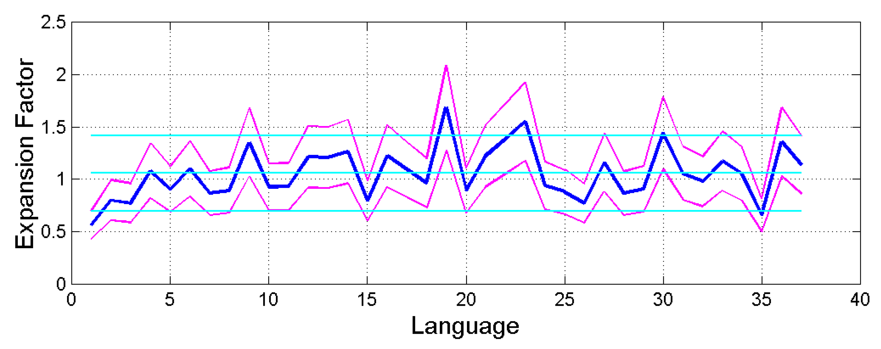
Figure 11.
Conditional mean (blue line) and 1–standard–deviation bounds (magenta lines) of
versus translation (for order number, see
Table 1). The cyan lines draw the overall mean and
standard deviation bounds;
samples per translation.
Figure 11.
Conditional mean (blue line) and 1–standard–deviation bounds (magenta lines) of
versus translation (for order number, see
Table 1). The cyan lines draw the overall mean and
standard deviation bounds;
samples per translation.
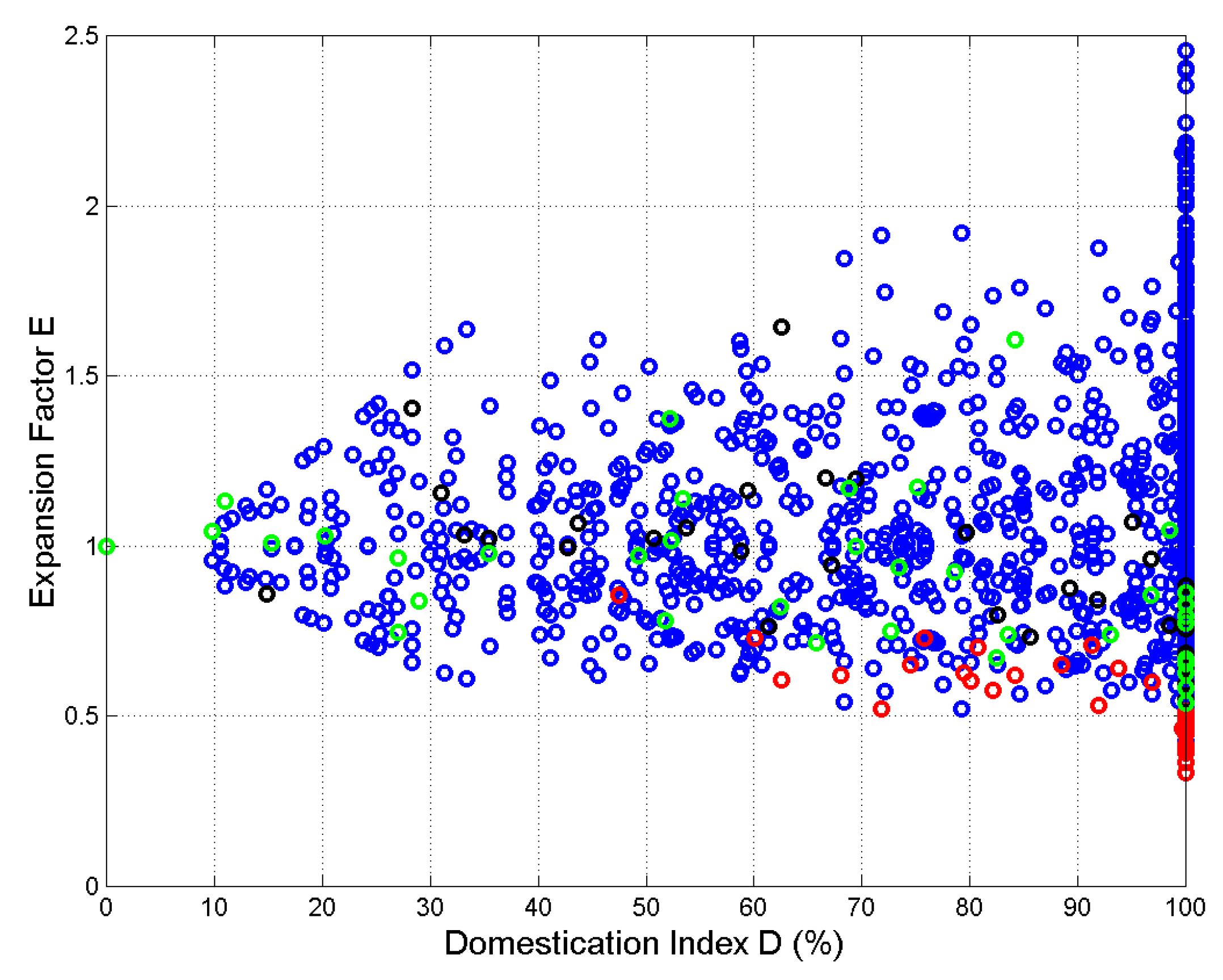
Figure 12.
Scatterplot of versus for all translations. The number of samples is . Reference language Greek, red circles; references language English, black circles; reference language Italian, green circles; all other languages, blue circles.
Figure 12.
Scatterplot of versus for all translations. The number of samples is . Reference language Greek, red circles; references language English, black circles; reference language Italian, green circles; all other languages, blue circles.
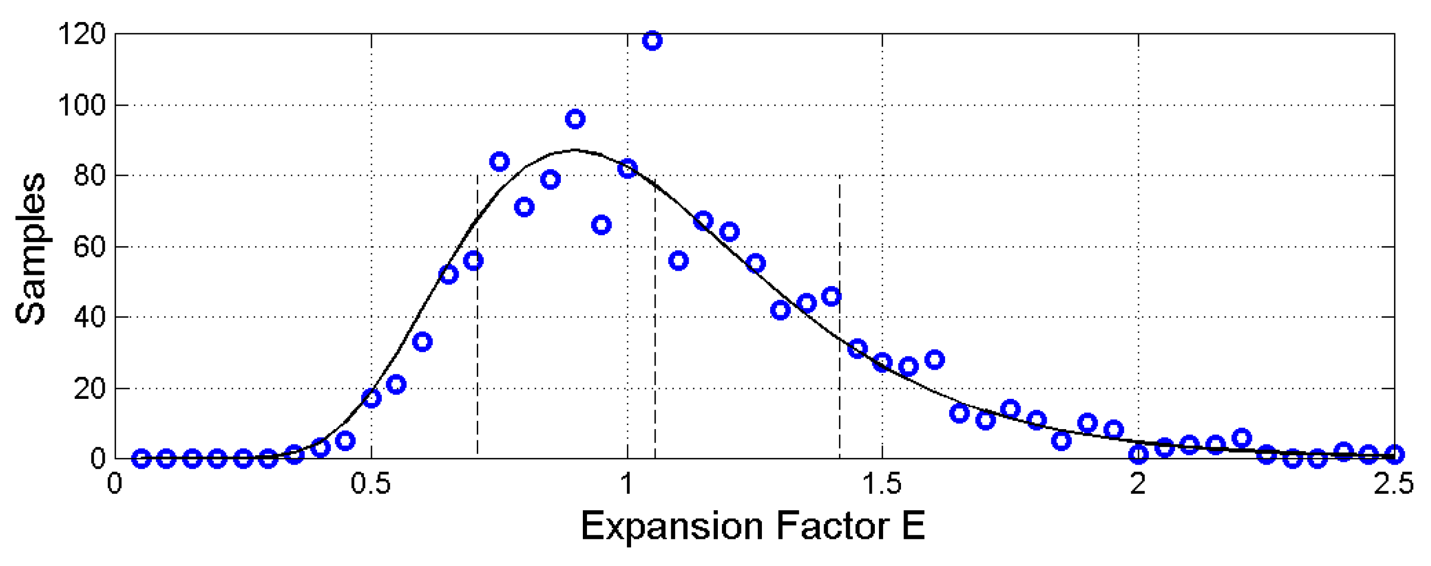
Figure 13.
Histogram of (blue circles) and its log–normal model (black line). The number of samples is The dash lines indicate standard deviations bounds.
Figure 13.
Histogram of (blue circles) and its log–normal model (black line). The number of samples is The dash lines indicate standard deviations bounds.
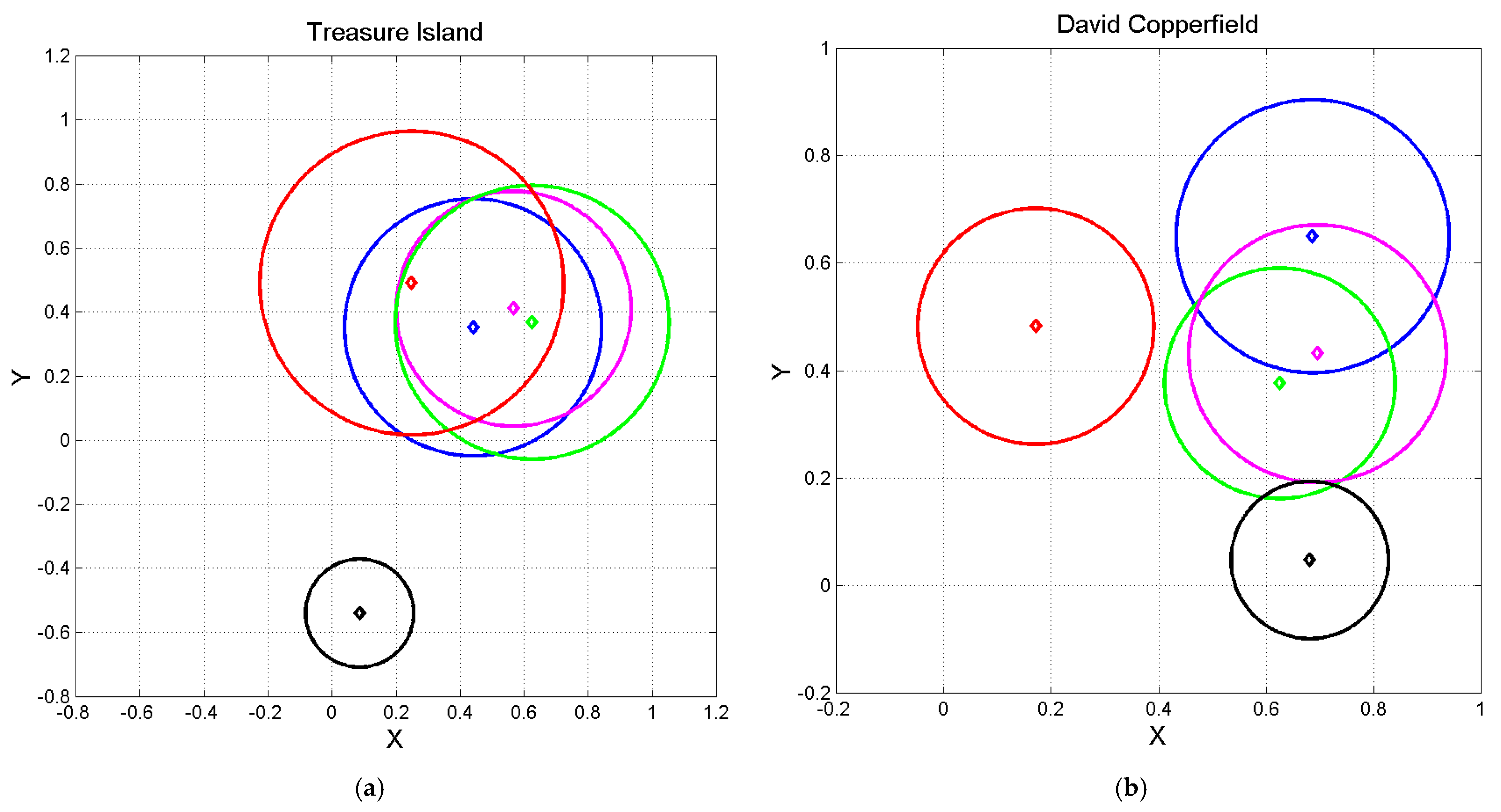
Figure 14.
Normalized coordinates
and
of the ending point of vector of Equation (6), calculated by setting
Haitian at the origin
and
Greek at
, red diamond, according to the linear tranformations (7) and (8). Circles with same color represent 1–sigma contour lines discussed in
Section 5. (
a)
Treasure Island. Color key: red, English; blue, French; green, Italian; magenta, German, black, Russian. (
b)
David Copperfield. Color key: English red; French blue, green, Italian; magenta, Spanish; black, Finnish.
Table 1.
Language of translation and language family of the New Testament books (
Matthew,
Mark,
Luke,
John,
Acts,
Epistle to the Romans, and
Apocalypse), with total number of characters (
, words (
, sentences (
), and interpunctions (
). The list concerning the genealogy of Jesus of Nazareth reported in
Matthew 1.1–1.17 17 and in
Luke 3.23–3.38 was deleted for not biasing the statistics of linguistic variables [
2,
4]. The source of the texts considered is reported in [
2].
| Language | Order | Abbreviation | Language Family | | | | |
|---|
| Greek | 1 | Gr | Hellenic | 486,520 | 100,145 | 4759 | 13,698 |
| Latin | 2 | Lt | Italic | 467,025 | 90,799 | 5370 | 18,380 |
| Esperanto | 3 | Es | Constructed | 492,603 | 111,259 | 5483 | 22,552 |
| French | 4 | Fr | Romance | 557,764 | 133,050 | 7258 | 17,904 |
| Italian | 5 | It | Romance | 505,535 | 112,943 | 6396 | 18,284 |
| Portuguese | 6 | Pt | Romance | 486,005 | 109,468 | 7080 | 20,105 |
| Romanian | 7 | Rm | Romance | 513,876 | 118,744 | 7021 | 18,587 |
| Spanish | 8 | Sp | Romance | 505,610 | 117,537 | 6518 | 18,410 |
| Danish | 9 | Dn | Germanic | 541,675 | 131,021 | 8762 | 22,196 |
| English | 10 | En | Germanic | 519,043 | 122,641 | 6590 | 16,666 |
| Finnish | 11 | Fn | Germanic | 563,650 | 95,879 | 5893 | 19,725 |
| German | 12 | Ge | Germanic | 547,982 | 117,269 | 7069 | 20,233 |
| Icelandic | 13 | Ic | Germanic | 472,441 | 109,170 | 7193 | 19,577 |
| Norwegian | 14 | Nr | Germanic | 572,863 | 140,844 | 9302 | 18,370 |
| Swedish | 15 | Sw | Germanic | 501,352 | 118,833 | 7668 | 15,139 |
| Bulgarian | 16 | Bg | Balto–Slavic | 490,381 | 111,444 | 7727 | 20,093 |
| Czech | 17 | Cz | Balto–Slavic | 416,447 | 92,533 | 7514 | 19,465 |
| Croatian | 18 | Cr | Balto–Slavic | 425,905 | 97,336 | 6750 | 17,698 |
| Polish | 19 | Pl | Balto–Slavic | 506,663 | 99,592 | 8181 | 21,560 |
| Russian | 20 | Rs | Balto–Slavic | 431,913 | 92,736 | 5594 | 22,083 |
| Serbian | 21 | Sr | Balto–Slavic | 441,998 | 104,585 | 7532 | 18,251 |
| Slovak | 22 | Sl | Balto–Slavic | 465,280 | 100,151 | 8023 | 19,690 |
| Ukrainian | 23 | Uk | Balto–Slavic | 488,845 | 107,047 | 8043 | 22,761 |
| Estonian | 24 | Et | Uralic | 495,382 | 101,657 | 6310 | 19,029 |
| Hungarian | 25 | Hn | Uralic | 508,776 | 95,837 | 5971 | 22,970 |
| Albanian | 26 | Al | Albanian | 502,514 | 123,625 | 5807 | 19,352 |
| Armenian | 27 | Ar | Armenian | 472,196 | 100,604 | 6595 | 18,086 |
| Welsh | 28 | Wl | Celtic | 527,008 | 130,698 | 5676 | 22,585 |
| Basque | 29 | Bs | Isolate | 588,762 | 94,898 | 5591 | 19,312 |
| Hebrew | 30 | Hb | Semitic | 372,031 | 88,478 | 7597 | 15,806 |
| Cebuano | 31 | Cb | Austronesian | 681,407 | 146,481 | 9221 | 16,788 |
| Tagalog | 32 | Tg | Austronesian | 618,714 | 128,209 | 7944 | 16,405 |
| Chichewa | 33 | Ch | Niger–Congo | 575,454 | 94,817 | 7560 | 15,817 |
| Luganda | 34 | Lg | Niger–Congo | 570,738 | 91,819 | 7073 | 16,401 |
| Somali | 35 | Sm | Afro–Asiatic | 584,135 | 109,686 | 6127 | 17,765 |
| Haitian | 36 | Ht | French Creole | 514,579 | 152,823 | 10,429 | 23,813 |
| Nahuatl | 37 | Nh | Uto–Aztecan | 816,108 | 121,600 | 9263 | 19,271 |
Table 2.
Mean and standard deviation of the normalized difference, (%), in Equation (1), for the indicated linguistic parameter.
Table 2.
Mean and standard deviation of the normalized difference, (%), in Equation (1), for the indicated linguistic parameter.
| | Characters | Words | Sentences | Interpunctions |
|---|
| Mean | 6.82 | 11.09 | 49.30 | 39.07 |
| Standard deviation | 15.99 | 2.14 | 26.71 | 17.43 |
Table 3.
Mean value (left number of column, ) and standard deviation (right number, ) of the surface deep–language parameters in the indicated language of the New Testament books (Matthew, Mark, Luke, John, Acts, Epistle to the Romans, and Apocalypse), calculated from 155 samples in each language. For example, in Greek, , with a standard deviation .
| Language | | | | |
|---|
| | | |
|---|
| Greek | 23.07 6.65 | 7.47 1.09 | 4.86 0.25 | 3.08 0.73 |
| Latin | 18.28 4.77 | 5.07 0.68 | 5.16 0.28 | 3.60 0.77 |
| Esperanto | 21.83 5.22 | 5.05 0.57 | 4.43 0.20 | 4.30 0.76 |
| French | 18.73 2.51 | 7.54 0.85 | 4.20 0.16 | 2.50 0.32 |
| Italian | 18.33 3.27 | 6.38 0.95 | 4.48 0.19 | 2.89 0.40 |
| Portuguese | 16.18 3.25 | 5.54 0.59 | 4.43 0.20 | 2.93 0.56 |
| Romanian | 18.00 4.19 | 6.49 0.74 | 4.34 0.19 | 2.78 0.65 |
| Spanish | 19.07 3.79 | 6.55 0.82 | 4.30 0.19 | 2.91 0.47 |
| Danish | 15.38 2.15 | 5.97 0.64 | 4.14 0.16 | 2.59 0.33 |
| English | 19.32 3.20 | 7.51 0.93 | 4.24 0.17 | 2.58 0.39 |
| Finnish | 17.44 4.09 | 4.94 0.56 | 5.90 0.31 | 3.54 0.75 |
| German | 17.23 2.77 | 5.89 0.60 | 4.68 0.19 | 2.94 0.45 |
| Icelandic | 15.72 2.58 | 5.69 0.67 | 4.34 0.18 | 2.77 0.39 |
| Norwegian | 15.21 1.43 | 7.75 0.84 | 4.08 0.13 | 1.98 0.22 |
| Swedish | 15.95 2.17 | 8.06 1.35 | 4.23 0.18 | 2.01 0.31 |
| Bulgarian | 14.97 2.61 | 5.64 0.64 | 4.41 0.19 | 2.67 0.43 |
| Czech | 13.20 3.10 | 4.89 0.65 | 4.51 0.21 | 2.71 0.61 |
| Croatian | 15.32 3.54 | 5.62 0.75 | 4.39 0.22 | 2.72 0.49 |
| Polish | 12.34 1.93 | 4.65 0.43 | 5.10 0.22 | 2.67 0.40 |
| Russian | 17.90 4.46 | 4.28 0.46 | 4.67 0.27 | 4.18 0.92 |
| Serbian | 14.46 2.42 | 5.81 0.69 | 4.24 0.20 | 2.50 0.39 |
| Slovak | 12.95 2.10 | 5.18 0.61 | 4.65 0.23 | 2.51 0.36 |
| Ukrainian | 13.81 2.18 | 4.72 0.41 | 4.56 0.26 | 2.95 0.58 |
| Estonian | 17.09 3.89 | 5.45 0.66 | 4.89 0.24 | 3.14 0.64 |
| Hungarian | 17.37 4.54 | 4.25 0.45 | 5.31 0.29 | 4.09 0.93 |
| Albanian | 22.72 4.86 | 6.52 0.78 | 4.07 0.22 | 3.48 0.61 |
| Armenian | 16.09 3.07 | 5.63 0.52 | 4.75 0.40 | 2.86 0.47 |
| Welsh | 24.27 4.75 | 5.84 0.44 | 4.04 0.15 | 4.16 0.76 |
| Basque | 18.09 4.31 | 4.99 0.52 | 6.22 0.27 | 3.63 0.81 |
| Hebrew | 12.17 2.04 | 5.65 0.59 | 4.22 0.17 | 2.16 0.33 |
| Cebuano | 16.15 1.71 | 8.82 1.01 | 4.65 0.10 | 1.85 0.22 |
| Tagalog | 16.98 3.24 | 7.92 0.82 | 4.83 0.17 | 2.16 0.44 |
| Chichewa | 12.89 1.79 | 6.18 0.87 | 6.08 0.18 | 2.10 0.25 |
| Luganda | 13.65 2.78 | 5.74 0.82 | 6.23 0.23 | 2.39 0.40 |
| Somali | 19.57 5.50 | 6.37 1.01 | 5.32 0.16 | 3.06 0.65 |
| Haitian | 14.87 1.83 | 6.55 0.71 | 3.37 0.10 | 2.28 0.26 |
| Nahuatl | 13.36 1.70 | 6.47 0.91 | 6.71 0.24 | 2.08 0.24 |
Table 4.
Synthesis of domestication index, (%), in the indicated translations. The column gives the number of translations that do not overlap with the language indicated in the first column. The other columns, for the language indicated in the first column, list the languages whose is in the indicated range, and the language with minimum, . In Latin, for example, 7 languages do not overlap; 7 languages overlap (Fr, It, Rm, Sp, Ge, Et, and Hn) in the range of ; and 5 languages overlap in the range of . The language with is Rm; the 18 languages not mentioned have . The language that is mostly not connected with the other languages is Nahuatl.
| | | | | |
|---|
| Greek | 18 | −− | Sm | Sm |
| Latin | 7 | Fr, It, Rm, Sp, Ge, Et, Hn | En, Fn, Sw, Ar, Sm | Rm |
| Esperanto | 17 | Al | Wl | Al |
| French | 13 | Lt, It, En | Rm, Sp, Fn, Hn, Sm | En |
| Italian | 9 | Lt, Fr, Rm, Sp, Ge, Et, Hn, | En, Fn | Rm |
| Portuguese | 9 | Dn, Ic, Cr | Ge, Bg, Sr, Rs, Et, Hn, Ar | Ic |
| Romanian | 7 | Lt, It, Sp, Ge, Et, Hn | Fr, En, Rs, Ar | It |
| Spanish | 9 | Lt, It, Rm | Fr, En, Hn | It |
| Danish | 14 | Pt, Ic, Bg, Cr, Sr | Ar | Ic |
| English | 12 | Fr, Sm | Lt, It, Sp, Fn, | Fr |
| Finnish | 10 | Sw, Bs | Lt, Fr, It, En, Tg, Sm | Sw |
| German | 10 | Lt, It, Rm, Et, Hn | Pt, Sp, Ar | Et |
| Icelandic | 10 | Pt, Dn, Bg, Cr | Sr, Ar | Dn |
| Norwegian | 9 | −− | Sw, Et, Ar | Sw |
| Swedish | 6 | Fn | Lt, Nr, Et, Bs, Tg | Fn |
| Bulgarian | 14 | Dn, Ic, Cr, Sr | Pt, Uk, Ar | Dn |
| Czech | 19 | Si, Uk, Hb | Pl, Sr, Ht | Uk |
| Croatian | 10 | Pt, Dn, Ic, Bg, Sr, Hb | Uk, Ar, Ht | Bg |
| Polish | 24 | Sl | Cz, Hb | Sl |
| Russian | 8 | −− | Pt, Rm, Et, Hn | Hn |
| Serbian | 14 | Dn, Bg, Cr | Pt, Ic, Cz, Sl, Uk, Ht | Bg |
| Slovak | 19 | Pl | Sr, Uk, Hb | Pl |
| Ukrainian | 16 | Cz | Bg, Cr, Sr, Sl, Ht | Cz |
| Estonian | 5 | Lt, It, Rm, Ge, Hn, Ar | Pt, Sp, Nr, Sw, Rs | Hn |
| Hungarian | 6 | Lt, It, Rm, Ge, Et | Fr, Pt, Sp, Rs, Ar | Et |
| Albanian | 19 | Es | Wl | Es |
| Armenian | 8 | Et | Pt, Rm, Dn, Ge, Ic, Nr, Bg, Cr, Hn | Et |
| Welsh | 26 | −− | Es, Al | Al |
| Basque | 14 | Fn, Tg, Sm | Sw, Cb | Tg |
| Hebrew | 25 | Cz | Pl, Sl | Cz |
| Cebuano | 18 | Tg | Bs | Tg |
| Tagalog | 16 | Bs, Cb | Fn, Sw, Sm | Bs |
| Chichewa | 27 | Lg | −− | Lg |
| Luganda | 25 | Ch | −− | Ch |
| Somali | 10 | En, Bs | Gr, Lt, Fr, Fn, Tg, | Bs |
| Haitian | 18 | −− | Cz, Cr, Sr, Uk | Uk |
| Nahuatl | 31 | −− | −− | Lg |
Table 5.
Treasure Island. Total number of characters (
, words (
, sentences (
), and interpunctions (
); and mean value (left number of column,
) and standard deviation (right number,
) of the deep–language parameters in the indicated versions. Notice that the values of
and
reported here differ from those reported in [
5], because in [
5], only sentences ending with full periods were considered.
| Language | | | | | | | | |
|---|
| | | |
|---|
| English | 273,717 | 68,033 | 3824 | 11,503 | 18.93 4.89 | 6.05 0.93 | 4.02 0.09 | 3.09 0.38 |
| French | 309,923 | 68,818 | 4054 | 11,443 | 17.80 4.08 | 6.11 0.80 | 4.50 0.14 | 2.88 0.33 |
| German | 349,955 | 72,119 | 4111 | 12,294 | 18.27 3.68 | 5.96 0.74 | 4.85 0.16 | 3.05 0.36 |
| Italian | 305,132 | 64,603 | 3805 | 10,077 | 17.92 4.33 | 6.52 0.86 | 4.72 0.12 | 2.72 0.37 |
| Russian | 265,428 | 54,142 | 5218 | 12,006 | 10.63 1.75 | 4.53 0.31 | 4.90 0.14 | 2.34 0.26 |
Table 6.
David Copperfield. Total number of characters (
, words (
, sentences (
), and interpunctions (
); and mean value (left number of column,
) and standard deviation (right number,
) of the deep–language parameters in the indicated versions. Notice that the values of
and
reported here differ from those reported in [
5], because in [
5], only sentences ending with full periods were considered.
| Language | | | | | | | | |
|---|
| | | |
|---|
| English | 1,468,884 | 363,284 | 19,610 | 64,914 | 18.83 2.50 | 5.61 0.30 | 4.04 0.12 | 3.35 0.33 |
| French | 1,700,735 | 366,762 | 18,456 | 54,770 | 20.21 2.62 | 6.73 0.49 | 4.64 0.08 | 3.00 0.26 |
| Italian | 1,596,684 | 334,864 | 18,919 | 52,367 | 17.97 2.27 | 6.42 0.39 | 4.77 0.10 | 2.80 0.26 |
| Spanish | 1,511,564 | 338,041 | 18,654 | 46,938 | 18.37 2.19 | 7.24 0.56 | 4.47 0.10 | 2.53 0.19 |
| Finnish | 1,764,033 | 295,564 | 19,614 | 65,270 | 15.25 1.67 | 4.55 0.18 | 5.97 0.14 | 3.36 0.28 |
Table 7.
Treasure Island. Domestication index, (%), in the indicated languages.
Table 7.
Treasure Island. Domestication index, (%), in the indicated languages.
| | English | French | German | Italian | Russian |
|---|
| English | 0 | 33.54 | 47.08 | 53.74 | 100 |
| French | 33.54 | 0 | 23.04 | 28.16 | 100 |
| German | 47.08 | 23.04 | 0 | 13.82 | 100 |
| Italian | 53.74 | 28.16 | 13.82 | 0 | 100 |
| Russian | 100 | 100 | 100 | 100 | 0 |
Table 8.
Treasure Island. Expansion factor, , in the indicated languages.
Table 8.
Treasure Island. Expansion factor, , in the indicated languages.
| | English | French | German | Italian | Russian |
|---|
| English | 1 | 1.18 | 1.29 | 1.11 | 2.80 |
| French | 0.85 | 1 | 1.09 | 0.94 | 2.38 |
| German | 0.77 | 0.91 | 1 | 0.86 | 2.17 |
| Italian | 0.90 | 1.07 | 1.16 | 1 | 2.52 |
| Russian | 0.36 | 0.42 | 0.46 | 0.40 | 1 |
Table 9.
David Copperfield. Domestication index, (%), in the indicated languages.
Table 9.
David Copperfield. Domestication index, (%), in the indicated languages.
| | English | French | Italian | Spanish | Finnish |
|---|
| English | 0 | 100 | 100 | 100 | 100 |
| French | 100 | 0 | 70.88 | 54.35 | 100 |
| Italian | 100 | 70.88 | 0 | 24.87 | 97.22 |
| Spanish | 100 | 54.35 | 24.87 | 0 | 99.94 |
| Finnish | 100 | 100 | 97.22 | 99.94 | 0 |
Table 10.
David Copperfield. Expansion factor, , in the indicated languages.
Table 10.
David Copperfield. Expansion factor, , in the indicated languages.
| | English | French | Italian | Spanish | Finnish |
|---|
| English | 1 | 0.86 | 1.02 | 0.92 | 1.50 |
| French | 1.16 | 1 | 1.18 | 1.06 | 1.73 |
| Italian | 0.98 | 0.84 | 1 | 0.90 | 1.46 |
| Spanish | 1.09 | 0.94 | 1.12 | 1 | 1.64 |
| Finnish | 0.67 | 0.58 | 0.68 | 0.61 | 1 |


